Article

Machine Learning in Classification Time Series with Fractal Properties †

by
Lyudmyla Kirichenko
1,
Tamara Radivilova
2,* and
Vitalii Bulakh
1
1
Department of Applied mathematics, Kharkiv National University of Radio Electronics, Kharkiv 61166, Ukraine
2
Department of Infocommunication Engineering, Kharkiv National University of Radio Electronics, Kharkiv 61166, Ukraine
*
Author to whom correspondence should be addressed.
This paper is an extended version of our conference paper: Bulakh, V., Kirichenko, L., Radivilova, T. Time Series Classification Based on Fractal Properties. In Proceedings of the 2018 IEEE Second International Conference on Data Stream Mining & Processing (DSMP), Lviv, Ukraine, 21–25 August 2018; pp. 198–201, doi:10.1109/DSMP.2018.8478532.
Submission received: 13 November 2018 / Revised: 18 December 2018 / Accepted: 23 December 2018 / Published: 28 December 2018
(This article belongs to the Special Issue Data Stream Mining and Processing)

Abstract

:
The article presents a novel method of fractal time series classification by meta-algorithms based on decision trees. The classification objects are fractal time series. For modeling, binomial stochastic cascade processes are chosen. Each class that was singled out unites model time series with the same fractal properties. Numerical experiments demonstrate that the best results are obtained by the random forest method with regression trees. A comparative analysis of the classification approaches, based on the random forest method, and traditional estimation of self-similarity degree are performed. The results show the advantage of machine learning methods over traditional time series evaluation. The results were used for detecting denial-of-service (DDoS) attacks and demonstrated a high probability of detection.

1. Introduction

Over the past two decades, machine learning methods for time series have been proposed and developed, which are used for many tasks of time series analysis, including classification [1,2,3,4]. The overview of classification methods of time series of different nature is described in [1]. The properties and characteristics of time series in emerging research that facilitates wide comparison of feature-based representations are given in [2]. The different machine learning algorithms were realized and compared by testing on 85 datasets in [3]. The authors of [4] describe the methods for mining time series data. Many complex technical and information systems have a fractal (self-similar) structure, and their dynamics is represented by time series with fractal properties [5]. For such systems, there are problems of recognition and classification of fractal series. Most often, they are solved by evaluation and analysis of self-similar properties. In recent years, machine learning methods became popular for analyzing and classifying fractal time series [6,7,8,9,10,11,12]. The authors of [6] conducted a systematic empirical study on the use of fractal dimension estimation methods as feature extractors from time series. A short literature review about fractal dimension on datasets and an approach to sentiment analysis with fractal dimension was presented in the work of [7]. Another paper [8] reported a novel method on the machine learning based classification of fractal features of time series using twin support vector machines. The authors of [9] demonstrated the successful application of the random forest method for predicting the Hurst parameter of precipitation records. A comparative analysis of the classification of multifractal stochastic time series using meta-algorithms based on decision trees has been performed by the authors of [10,11], where the features for classification were statistical and multifractal characteristics. The authors of [12] reviewed the most recent theoretical and methodological developments for random forests with special attention given to the selection of parameters, the resampling mechanism, and variable importance measures.
An actual machine learning application is the timely detection of distributed denial-of-service (DDoS) attacks. A DDoS attack is a hacker attack on a computing system; in this case, administrators (and users) cannot get access to the system. Currently, DDoS attacks are very popular, as they allow one to bring to failure almost any system without leaving legally relevant evidence. One of the solutions to the problem of detecting an attack in a timely manner is to develop a classifier that is able to detect the presence of attacking files in incoming traffic. It is known that most of the traffic in infocommunication systems has fractal properties [13]. Plenty modern methods of detecting DDoS attacks are based on the fact that fractal properties change for traffic containing attacking files [14,15,16,17]. In another paper [14], the authors have tried to measure the impact of different variants of pulsating distributed denial of service attacks on the self-similar nature of the network traffic and have shown that the variation in self-similar properties could be used for distinguishing them from normal network traffic. The authors of [15] show that the self-similarity property of network traffic is useful in distinguishing DDoS attack traffic from legitimate traffic with high accuracy. The authors of [16] describe a statistical signal processing technique based on abrupt change detection using self-similar traffic properties. The time series fractal analysis methods, and random forest method were used to detect anomalies in network traffic [17].
The aim of the work is a comparative analysis of decision tree classification methods for fractal random time series and the application of the results in detecting DDoS attacks.

2. Materials and Methods

2.1. Characteristics and Models of Fractal Random Processes

Self-similar processes are stochastic processes that are invariant in distribution when changing the time-scale. A random continuous time process X ( t ) is self-similar if its finite-dimensional distributions are identical distributions of the process a H X ( a t ) for any a > 0 . The value H is called the Hurst parameter or Hurst exponent. The Hurst exponent takes values in the range 0 < H < 1 . The H also characterizes the long-term memory of the process X ( t ) . The moments of the self-similar random process are described by the scaling relation:
E [ | X ( t ) | q ] t q H
where q is a real number.
Multifractal random processes are heterogeneous fractal processes. The moments of the multifractal process satisfy more a flexible scaling relation:
E [ | X ( t ) | q ] t q h ( q )
where h ( q ) is the generalized Hurst exponent. The Hurst exponent H matches the value of the generalized Hurst exponent h ( 2 ) . For monofractal time series, the generalized Hurst exponent is constant, h ( q ) = H [18].
Popular multifractal time series models are binomial multiplicative stochastic cascade processes [18]. When constructing stochastic cascades, the initial unit time interval is first divided into two equal sub-intervals. Each of them is assigned corresponding weight coefficients w 1 and 1 w 1 , which are values of some random variable. At each iteration, the sum of the weighting coefficients must be equal to one. If you choose a random variable distributed on the interval [ 0 , 1 ] , this constraint will be satisfied. At the next iteration, two new random values are generated. There are four sub-intervals with weights w 1 w 2 , w 1 ( 1 w 2 ) , ( 1 w 1 ) w 3 , and ( 1 w 1 ) ( 1 w 3 ) . By increasing the number of iterations, we get a cascade time series, the values of which at each time are equal to the final simulated weights. The cascade time series has multifractal properties.
If the beta distribution random variable B e t a ( α , β ) is used to generate weights, then the generalized Hurst exponent of cascade is uniquely determined by the parameters α and β [18,19]. Thus, each given pair ( α , β ) corresponds to the cascade process with a single Hurst exponent H .
Figure 1 shows a typical cascade time series based on beta distribution; on the top, the cascade series with H = 0.7 is presented, and on the bottom, there is the cascade with H = 0.9 .
In recent years, research of the fractal analysis of information network traffic has become very popular. They indicate that most of the traffic has multifractal properties [13]. In the work of [19], the method of simulating multifractal traffic based on cascades with beta distribution was offered.

2.2. Time Series Estimation of Fractal Characteristics

There are many time series methods for the evaluation of fractal characteristics. One of the most well-known and widespread is the method of multifractal detrended fluctuation analysis (MFDFA) [20]. Previous large-scale research, which assessed the performance of the Hurst estimator [21,22,23], has demonstrated that the detrended fluctuation analysis (DFA) is an accurate estimator. DFA has been established as an important method to detect long-range dependence in non-stationary time series. MFDFA is an extension of the DFA to analyze the multifractal properties of time series with nonstationary dynamics and different distributions of values [24]. DFA and MFDFA are widely used for applied research [6,12,25,26,27].
According to DFA method, input cumulative time series y ( t ) is divided into segments of length τ . For each segment, the fluctuation function F 2 ( τ ) = 1 τ t = 1 τ ( y ( t ) Y m ( t ) ) 2 is calculated, where Y m ( t ) is a local m-polynomial trend within the segment. Then, the fluctuation function F ( τ ) is averaged over the segments. If the series y ( t ) is self-similar, the function F ( τ ) satisfies the scaling relation F ( τ ) τ H .
In the case of multifractal fluctuation analysis, the fluctuation function F q ( τ ) = { 1 N i = 1 N [ F 2 ( τ ) ] q 2 } 1 q is explored. If the initial time series y ( t ) has multifractal properties, the function F q ( τ ) satisfies the scaling relation F q ( τ ) τ h ( q ) .
The time series estimation of the Hurst parameter results in a confidence interval:
H t α S < H < H + t α S
where H = H ( N ) is a point estimate of H , N is the length of the time series, S = S ( N ) is the calculated standard deviation, α is the significance level, and t α is a normal distribution quantile. Values S can be numerically evaluated based on simulation. It should be noted the magnitude of the uncertainty in the estimation of H also depends on the value of H . This is shown in a number of studies, for example [25,27]. However, for the estimates obtained by the DFA method, the bias is not significant and in the present study, it is not taken into account to simplify computational issues.
Table 1 shows values S for the estimates of the Hurst exponent obtained by the DFA [26,27].

2.3. Time Series Classification Using Decision Tree Methods

To solve classification problems that arise in various areas, the decision tree method is considered as one of the most effective methods. Its core is splitting the initial dataset into groups of homogeneous subsets. This splitting is based on a set of rules, which is used to evaluate some input functions for new data and allows making the relevant classification conclusion.
The decision tree method uses the recursive partitioning principle. There are various numerical algorithms for building decision trees. One of the most famous is the C5.0 algorithm [28], which is practically standard for building a binary tree based on some criterion for splitting into more homogeneous samples. The algorithm implements the recursive partitioning method. It starts with an empty tree and source data set. Starting from the root node, a feature is selected at the nodes, the value of which is used to split data according to a certain criterion into two disjoint subsets. The iteration process is performed repeatedly for each of the subsets and leads to the creation of a complete binary tree. Recursion is completed if the subset in the node has the same values of the target variable.
The decision tree models are unstable because they adapt their state in the learning process in accordance with the training set: the tree structure changes with any tiny changes in the set. This implies that we will always get a different model when making minor changes in training data. However, the modified and original models work similarly and with comparable accuracy: the basic regularities are not changeable with minor changes in the training data. In this case, it is desirable to use model ensembles. In general, the model’s ensemble can be seen as an individual basic model making up a common model. The components of the ensemble can be different or of the same type.
The bagging method based on the statistical method of aggregation of the boot system is one of the most well-known types of ensembles [29]. Bootstrap aggregating reduces variance and helps to avoid retraining. This method is designed for improving the stability and accuracy of machine learning algorithms. Bagging is a classification technique in which all elementary classifiers study and work independently. The main idea is that the classifiers compensate for each other’s mistakes by voting and not correcting them. The “perturbation and combination classification” technology is the basis of the bagging method. In bagging, the random changes are involved in the training data. Then, based on these modified data, several alternative models are constructed. After this, a combination of results is considered. From one training set, several samples are randomly selected with the same number of objects. For training of an ensemble model, each of the samples is applied. If an ensemble is built based on various type models, then each type has its own learning algorithm.
To obtain the result of the model ensemble, the main combinational methods are used, such as the averaging method, which average results of all these models (when performing weighted averaging, the model outputs are multiplied by the corresponding weights); and the voting method (a class that had been elected by a majority of ensemble models). The efficiency of bagging is achieved because of the fact that the objects of emission cannot be included in some training subsamples, and the basic algorithms, trained in different subsamples, are obtained quite differently, and their errors are mutually compensated in the voting process.
One example of the bagging methods is the random forest method [30]. The key point of the random forest method is the way in which the training samples for decision trees are generated. It includes a random selection of fewer features for each training sample (that is, for each tree) and a random selection of training examples (thus some examples are repeated, and some are missing in the training set for a particular tree). It has several advantages against its main version: (1) within itself, it uses classification or regression decision tree ensembles; (2) the decision tree is built for each subsample to complete the object’s training and is not subject to post pruning; (3) in the sampling algorithm, random function selection of features is also sampling carried (in most cases, the new number of functions is equal to the square root of the total number), as well as the random selection of learning objects.

3. Results and Discussion

Experiment 1: bagging versus random forest and classification trees versus regression trees.
At the first stage, a study was conducted in order to single out the model with the highest probability of the class determination of time series. The classification was performed for time series with different multifractal properties. Training time series for the experiment were obtained by the generation of multifractal cascades with weights obtained by symmetric beta distribution. Under these conditions, the model fractal series contain the Hurst exponent in the range H ( 0.5 , 1 ) , and the Hurst exponent corresponds one-by-one to the generalized Hurst exponent h ( q ) . Therefore, the set time series can be partitioned into classes with respect to the value of H.
In this case, each class was a set of generated time series with the same Hurst exponent. The Hurst exponent value varied in the range from 0.5 to 1 with a step of 0.05. The minimum and maximum values of the Hurst exponent were selected as 0.51 and 0.99, respectively. As a result, classification models were trained in 11 classes.
The following fractal and statistical characteristics of time series were selected for the classification: maximum value and median of series, standard deviation, the mean and standard deviation of the generalized Hurst exponent h ( q ) , the values h ( 1 ) and h ( 2 ) = H , and the range Δ h = h ( 0.1 ) h ( 5 ) . Thus, in the experiment, cascade time series were selected as objects, and the estimates of time series characteristics of each cascade were chosen as the features.
To detect to which one of the eleven classes the time series belongs to, the methods of bagging and random forest were applied. For each of the methods, the ensembles of decision trees, both classifications and regressions, were used. For regression decision trees, the output is the probability of matching the multifractal cascade to a given class. The programming language Python with NumPy SciPy, Pandas, and Scikit-learn libraries, which implement machine learning methods, was chosen to implement the decision tree models [31].
When performing the experiment, the number of bootstrap samples was taken in the range from 200 to 500 in increments of 50. The best results on the test sample were obtained when the number of bootstrap samples was 300. The number of candidates sampled randomly at each split was equal to the square root of the total number of features. The minimum node size of the tree was chosen equal to 1, because regression trees were used for the classification task. For determining the optimal parameters of the method, good accuracy was achieved on the validation sample and the lack of overfitting, that is, when on the training sample, the accuracy was almost equal to 1, and on the test sample, it was close to 0.5 [32].
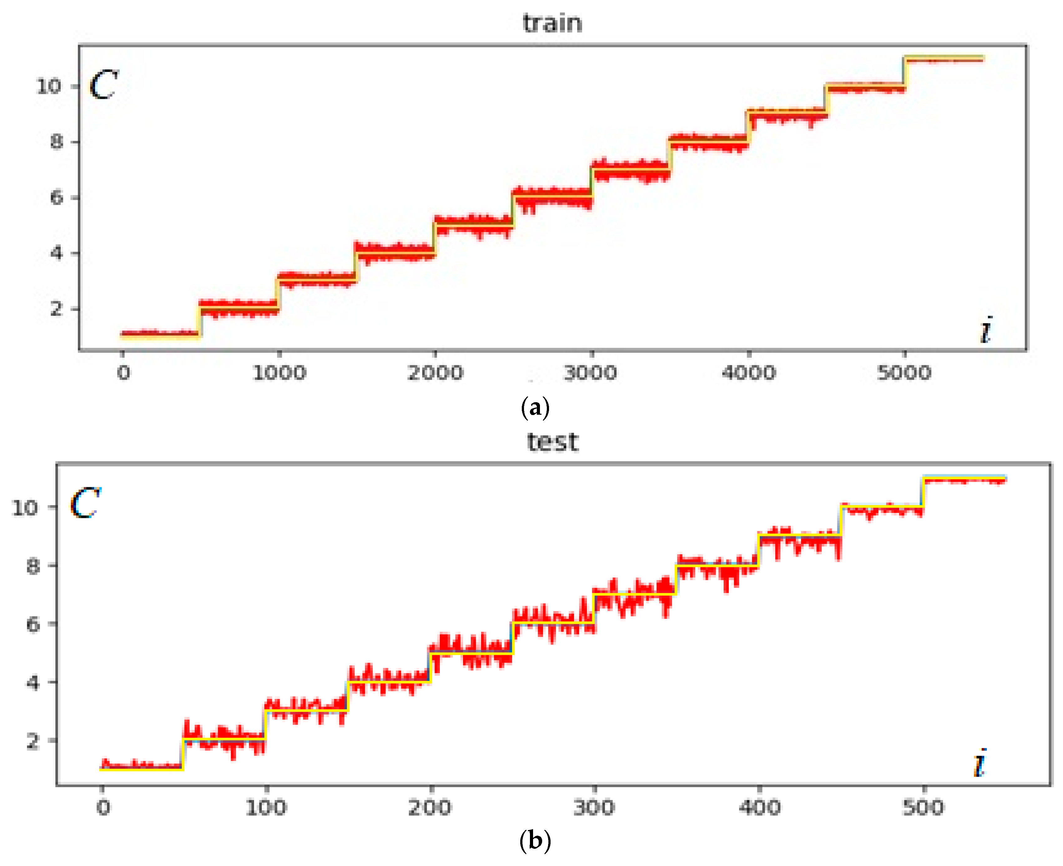
Figure 2 illustrates the effectiveness of the training model by the bagging method with regression trees. Each step corresponds to one class C = 1 , ,   11 . For each class, the probabilities of matching are given. The probabilities are calculated as follows:
P i = 1 | m i C |
where m i is the regression parameter for the i-th sample and C is a theoretically known number. If the condition P i [ 0.5 ; 1 ] holds, the classification is considered correct. If P i < 0.5 and m i > C , then the cluster number is overvalued. Otherwise, it is underestimated. In Figure 2, the top graph shows the results of modeling on a training sample of 5000 examples. The lower graph shows similar results for 500 test examples. Here, the length of the time series is 4096 values.
Table 2 presents the average probabilities of the class determination depending on the time series length and the classification method. The probability of the class determination is the probability of correct determination of the range of the Hurst exponent, corresponding to the theoretical value of H of generated cascade.
The results show that the use of regression trees gave significantly greater accuracy than the use of classification trees. The random forest method demonstrated better results than bagging. The simulation results match the theoretical studies [33], and the comparison of bagging and random forests is a good illustration of the theory. Therefore, for the classification, the random forest method with regression trees was chosen.
Experiment 2: machine learning versus estimation by time series.
To determine the class to which a time series belongs to, two different approaches were considered in the section. The first method of multifractal cascade series classification is based on machine learning, and the second method uses a direct estimation of the Hurst exponent for time series and determines the confidence interval in accordance with formula (3).
In the experiment, each class was represented by a set of simulated cascade time series with the Hurst parameter of a certain range of values. The value of H is chosen to generate cascades within each class using a uniform distribution. To create series classes, the ranges of the Hurst exponent were varied in the interval (0.5, 1) with increments of 0.05. The minimum values of H were chosen at the level of 0.51 and the maximum at the level of 0.99. The eleven classes were used to train the models with H ∈ {[0.51, 0.525], [0.525, 0.575], [0.575, 0.625] … [0.975, 0.99]}.
The input date classifier is a set of characteristics calculated from the cascade time series. The output parameter is the class number, that is, the range of the Hurst exponent. The following fractal and statistical characteristics of the time series were selected for the classification: maximum value and median of series, standard deviation, the mean and standard deviation of the generalized Hurst exponent h ( q ) , the values h ( 1 ) and h ( 2 ) = H , and the range Δ h = h ( 0.1 ) h ( 5 ) . Thus, in the experiment, cascade time series were selected as objects, and the estimates of time series characteristics of each cascade were chosen as the features. The random forest using regression decision trees method was chosen for the classification. The probabilities of class detecting were calculated by formula (4). To build the models of a decision tree, Python libraries, which implement machine learning methods, were used. The training of the models for each class was conducted on 1000 examples of time series, and the test was carried out on 100 test cases.
In a second way (direct estimation), the classification was performed for the same test sample series. Point estimates of the Hurst exponent were obtained by the DFA method and confidence intervals were calculated in accordance (3). The matching of the time series to one of the classes was determined using the location confidence interval. The class number is the number of the Hurst exponent range that contains most of the distribution density of the interval estimate.
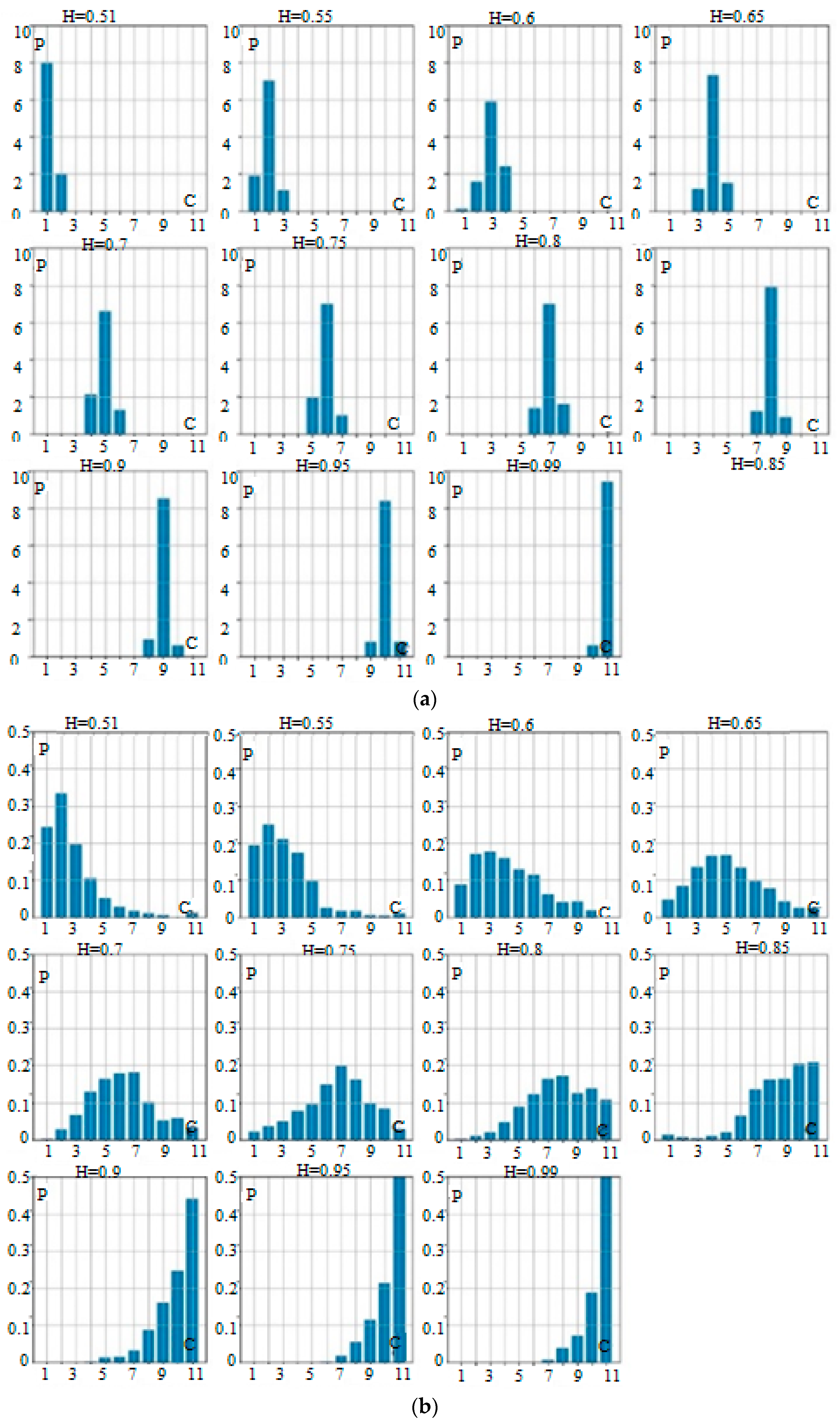
As a classification result, for each range of the Hurst exponent, the histograms of the probabilities of class determination were obtained. Figure 3 shows the histograms of the probability distribution of matching to a particular class. Histograms of the results of random forest are presented on the left, and histograms obtained by a direct estimation are on the right. Here, the length of the time series is 512 values.
The classification was performed for time series with lengths of 512 and 4096 values, then results were compared. Poor quality of the classification, or rather the inability to classify fractal series by time series estimation, is the result of the narrow range of the Hurst exponent for each class and the sufficiently large value of the confidence interval (see Table 1).
In many classification tasks, it is required to determine the probability that an object belongs to one of two classes (e.g., to detect an attack on a server). The classification of the cascade series into two classes was conducted. The Hurst exponent was chosen in two ranges: 0.51 H < 0.7 and 0.7 H 0.99 .
The average probability of class determination depending on the classification method is shown in Table 3. As can be seen from the table, to a large extent, traditional methods for evaluating fractal characteristics are inferior to machine learning methods when classifying time series according to fractal properties. However, it should be noted that for the training, a sufficient number of time series with known properties is required, which may be challenging.
Experiment 3: detecting DDoS-attacks.
This section presents the results of detecting DDoS attacks based on the random forest classification using regression decision trees. The objects were the model traffic realizations with attacks and without them. The simulation of traffic realizations was performed using the algorithm from the work of [19]. To generate a model traffic realization, it is necessary to estimate the following parameters of real multifractal telecommunication traffic: the average of the traffic; the Hurst exponent, which determines the degree of long-range dependence; and the scaling exponent, which determines the heterogeneity (bursts) of realization. Thereafter, beta distribution parameters for generating weighting coefficients of the multifractal cascade are selected. The matching between the distribution parameters and the multifractal characteristics was obtained as a result of numerical simulation.
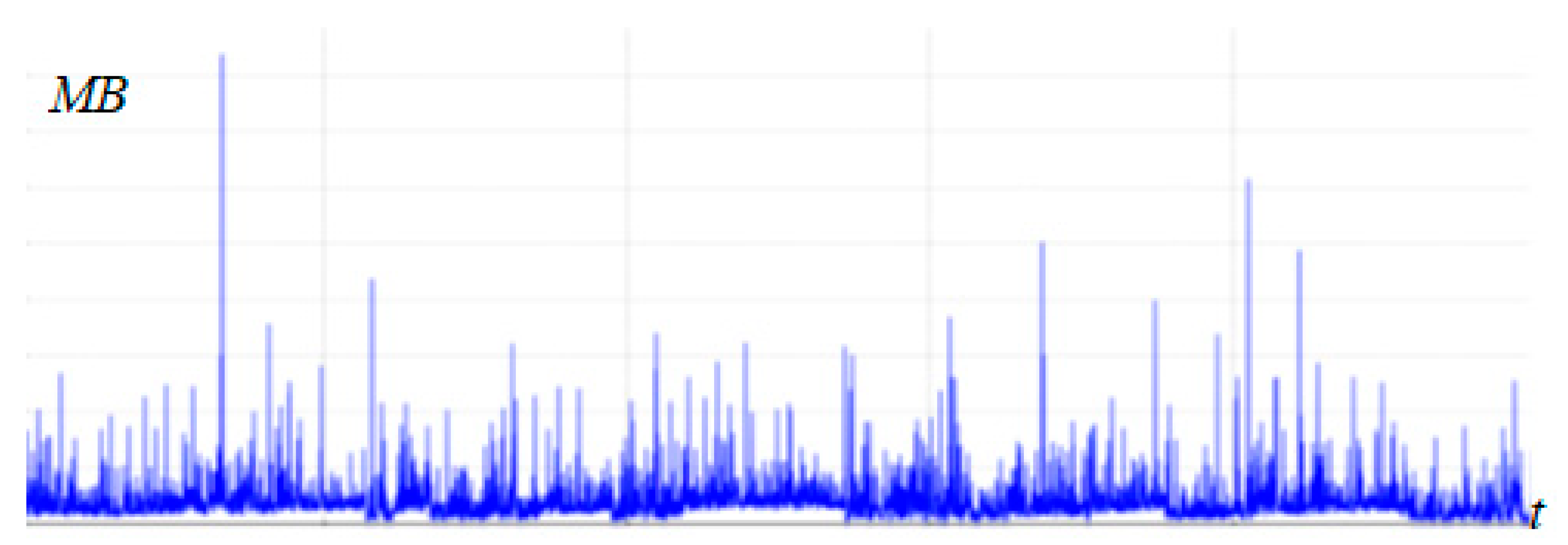
The mechanism for collecting real statistical data of DDoS attacks and examples of their application are presented in the work of [34]. Real experiments were conducted in which six types of realizations of DDoS attacks and brute force attacks were obtained. The dataset consists of 4998 records, where each record consists of 34 databases of management variables called management information base (MIB), which are collected in their respective groups; namely, interface, internet protocol (IP), transmission control protocol (TCP), and internet control message protocol (ICMP). Experiments and datasets are described in detail in the work of [34]. Figure 4 shows several attacks from the dataset.
The realization of traffic under the action of DDoS attack is the sum of traffic and realization of one type of attack. The early detection of an attack is highly important, when the realization of traffic has not yet faced a significant trend change. In this case, the ratio of the traffic average to the attack average was taken approximately in the 5:4 range. Figure 5 presents a realization with an attack level of 15%.
In the works of [35,36], it was shown that a self-similar time series, which is the sum of several self-similar series, acquires the highest Hurst exponent. The fractal analysis of the realizations of DDoS attacks showed that the attacks presented in [34] have a large range of the generalized Hurst exponent h ( q ) and high H values. Thus, the attacked traffic, as the sum of two self-similar time series with different fractal characteristics, has a higher Hurst exponent H and larger range changes h ( q ) than normal traffic. In this case, we can use the classification methods discussed above.
The partitioning of time series into two classes was performed. The first class was the set of realizations of model traffic based on a multifractal cascade, while the second one was the set of thee corresponding realizations of attacked traffic, that is, the sum of traffic and an attack. To generate traffic within each class, values of H were chosen that were uniformly distributed in a certain range.
The random forest using regression decision trees method was chosen as a classification method. The output of the model operation was the probability of attack detection. For the classification, statistical and multifractal characteristics obtained from time series were used. Thus, the objects were model traffic realizations (with or without attack), and the features were the characteristics estimates calculated for each realization.
For software implementation of the classification, Python was used with libraries that implement machine learning methods. Model training for each class was performed on 1000 examples of time realizations of training and tested on 100 test cases. The classification was carried out for traffic realizations of different lengths, while for comparing the results, the focus was on realizations of 4096 values.
In a numerical experiment, the detection was carried out for model traffic with different ranges of the Hurst exponent, which may correspond to the traffic of different types or different protocols. Table 4 shows the average probability of determining the attack depending on the value of the Hurst parameter for model traffic.
Table 4 clearly shows that the lower the Hurst rate of traffic, the higher the probability of detecting an attack. This is easily explained by the fact that the attacked traffic has much stronger self-similar and multifractal properties, and, accordingly, more differences in the class range.

4. Conclusions

In this paper, a comparative analysis of different approaches to classification of fractal random time series was conducted. Meta-algorithms based on decision trees were chosen for the classification. Objects of the classification were binomial multiplicative stochastic cascade time series, which were partitioned into classes depending on their Hurst exponent.
The classification was performed using two contrasting approaches. In the first, it was conducted using the random forest method using fractal and statistical characteristics of the time series. In the second case, the probability of matching to the class was calculated by time series estimating the Hurst exponent. The classification results demonstrated the indisputable advantage of machine learning methods over the habitual methods of evaluating the Hurst parameter.
The results were used for detecting DDoS attacks, indicating that the machine learning methods, particularly the random forest method, can be successfully applied for detecting DDoS attacks. The probability of attack detection highly depends on the value of the Hurst parameter of traffic realization and decreases as it increases.
It is necessary to emphasize that the use of machine learning is possible if there is a sufficiently large amount of training data, which is intractable in many cases. Also, an interesting and promising task is to develop classification methods for application in the generation of time series with prerequired properties and real data as a training sample.
In future research, we intend to focus on the investigation and classification of traffic of various transmission protocols, such as DDoS attacks of different types, in order to develop methods of early intrusion detection.

Author Contributions

Data curation, T.R.; Investigation, T.R.; Methodology, T.R.; Resources, V.B.; Software, V.B.; Supervision, L.K.; Validation, V.B.; Writing—original draft, L.K.

Funding

This research received no external funding.

Acknowledgments

In this section you can acknowledge any support given which is not covered by the author contribution or funding sections. This may include administrative and technical support, or donations in kind (e.g., materials used for experiments).

Conflicts of Interest

The authors declare no conflict of interest.

References

  1. Esling, P.; Agon, C. Time series data mining. ACM Comput. Surv. 2012, 45, 12:1–12:34. [Google Scholar] [CrossRef]
  2. Ben, D. Feature-Based Time-Series Analysis. 2017. Available online: https://arxiv.org/abs/1709.08055 (accessed on 26 October 2018).
  3. Bagnall, A.; Lines, J.; Bostrom, A.; Large, J.; Keogh, E. The great time series classification bake off: A review and experimental evaluation of recent algorithmic advances. Data Min. Knowl. Discov. 2017, 31, 606–660. [Google Scholar] [CrossRef]
  4. Kirichenko, L.; Radivilova, T.; Zinkevich, I. Comparative Analysis of Conversion Series Forecasting in E-commerce Tasks. In Advances in Intelligent Systems and Computing II. CSIT 2017; Shakhovska, N., Stepashko, V., Eds.; Springer: Cham, Switzerland, 2018; Volume 689, pp. 230–242. [Google Scholar] [CrossRef]
  5. Brambila, F. Fractal Analysis—Applications in Physics, Engineering and Technology. Available online: https://www.intechopen.com/books/fractal-analysis-applications-in-physics-engineering-and-technology (accessed on 28 October 2018).
  6. Coelho, A.L.V.; Lima, C.A.M. Assessing fractal dimension methods as feature extractors for EMG signal classification. Eng. Appl. Artif. Intell. 2014, 36, 81–98. [Google Scholar] [CrossRef]
  7. Symeon, S. Sentiment analysis via fractal dimension. In Proceedings of the 6th Symposium on Future Directions in Information Access, Thessaloniki, Greece, 2 September 2015; pp. 48–50. [Google Scholar] [CrossRef]
  8. Arjunan, S.P.; Kumar, D.K.; Naik, G.R. A machine learning based method for classification of fractal features of forearm sEMG using Twin Support vector machines. In Proceedings of the 2010 Annual International Conference of the IEEE Engineering in Medicine and Biology, Buenos Aires, Argentina, 31 August–4 September 2010; pp. 4821–4824. [Google Scholar] [CrossRef]
  9. Tyralis, H.; Dimitriadis, P.; Koutsoyiannis, D.; O’Connell, P.E.; Tzouka, K.; Iliopoulou, T. On the long-range dependence properties of annual precipitation using a global network of instrumental measurements. Adv. Water Resour. 2018, 111, 301–318. [Google Scholar] [CrossRef]
  10. Bulakh, V.; Kirichenko, L.; Radivilova, T. Classification of Multifractal Time Series by Decision Tree Methods. In Proceedings of the 14th International Conference ICTERI 2018 ICT in Education, Research, and Industrial Applications, Kyiv, Ukraine, 14–17 May 2018; pp. 1–4. [Google Scholar]
  11. Bulakh, V.; Kirichenko, L.; Radivilova, T. Time Series Classification Based on Fractal Properties. In Proceedings of the 2018 IEEE Second International Conference on Data Stream Mining & Processing (DSMP), Lviv, Ukraine, 21–25 August 2018; pp. 198–201. [Google Scholar] [CrossRef]
  12. Biau, G.; Scornet, E. A random forest guided tour. TEST 2016, 25, 197–227. [Google Scholar] [CrossRef]
  13. Shelukhin, O.I.; Smolskiy, S.M.; Osin, A.V. Self-Similar Processes in Telecommunications; John Wiley & Sons: New York, NY, USA, 2007; 320p. [Google Scholar]
  14. Kaur, G.; Saxena, V.; Gupta, J. Detection of TCP targeted high bandwidth attacks using self-similarity. J. King Saud Univ. Comput. Inf. Sci. 2017. [Google Scholar] [CrossRef]
  15. Deka, R.; Bhattacharyya, D. Self-similarity based DDoS attack detection using Hurst parameter. Secur. Commun. Netw. 2016, 9, 4468–4481. [Google Scholar] [CrossRef]
  16. Popa, S.M.; Manea, G.M. Using Traffic Self-Similarity for Network Anomalies Detection. In Proceedings of the 2015 20th International Conference on Control Systems and Computer Science, Bucharest, Romania, 27–29 May 2015; pp. 639–644. [Google Scholar] [CrossRef]
  17. Bulakh, V.; Kirichenko, L.; Radivilova, T.; Ageiev, D. Intrusion Detection of Traffic Realizations Based on Maching Learning using Fractal Properties. In Proceedings of the 2018 International Conference on Information and Telecommunication Technologies and Radio Electronics (UkrMiCo), Odessa, Ukraine, 10–14 September 2018; pp. 1–4. [Google Scholar]
  18. Riedi, R.H. Multifractal Processes. Available online: https://www.researchgate.net/publication/2839202_Multifractal_Processes (accessed on 27 December 2018).
  19. Kirichenko, L.; Radivilova, T.; Kayali, E. Modeling telecommunications traffic using the stochastic multifractal cascade process. Radio Electron. Comput. Sci. Control 2012, 55–63. [Google Scholar] [CrossRef]
  20. Kantelhardt, J. W.; Zschiegner, S. A.; Koscielny-Bunde, E.; Havlin, S.; Bunde, A.; Stanley, H.E. Multifractal detrended fluctuation analysis of nonstationary time series. Phys. A Stat. Mech. Its Appl. 2002, 316, 87–114. [Google Scholar] [CrossRef] [Green Version]
  21. Taqqu, M.; Teverovsky, V.; Willinger, W. Estimators for long-range dependence: An empirical study. Fractals 1995, 3, 785–798. [Google Scholar] [CrossRef]
  22. Tyralis, H.; Koutsoyiannis, D. Simultaneous estimation of the parameters of the Hurst–Kolmogorov stochastic process. Stoch. Environ. Res. Risk Assess. 2011, 25, 21–33. [Google Scholar] [CrossRef]
  23. Rea, W.; Oxley, L.; Reale, M.; Brown, J. Estimators for long range dependence: An empirical study. Electron. J. Stat. 2009. Available online: https://arxiv.org/pdf/0901.0762.pdf (accessed on 10 December 2018).
  24. Kantelhardt, J.W. Fractal and Multifractal Time Series. 2008. Available online: https://arxiv.org/abs/0804.0747 (accessed on 2 December 2018).
  25. Tyralis, H.; Koutsoyiannis, D. A Bayesian statistical model for deriving the predictive distribution of hydroclimatic variables. Clim. Dyn. 2014, 42, 2867–2883. [Google Scholar] [CrossRef]
  26. Kirichenko, L.; Radivilova, T.; Bulakh, V. Generalized approach to Hurst exponent estimating by time series. Inform. Autom. Pomiary Gospod. Ochr. Środowiska 2018, 8, 28–31. [Google Scholar] [CrossRef]
  27. Kirichenko, L.; Radivilova, T.; Deineko, Z. Comparative Analysis for Estimating of the Hurst Exponent for Stationary and Nonstationary Time Series. Inf. Technol. Knowl. 2011, 5, 371–388. [Google Scholar]
  28. Quinlan, J.R. C4.5: Programs for Machine Learning; Morgan Kaufmann Publishers Inc.: San Francisco, CA, USA, 1993; 302p. [Google Scholar]
  29. Breiman, L. Bagging predictors. Mach. Learn. 1996, 24, 123–140. [Google Scholar] [CrossRef] [Green Version]
  30. Breiman, L. Random Forests. Mach. Learn. 2001, 45, 5–32. [Google Scholar] [CrossRef] [Green Version]
  31. Cielen, D.; Meysman, A.; Ali, M. Introducing Data Science: Big Data, Machine Learning, and More, Using Python Tools; Manning Publications: Shelter Island, NY, USA, 2016; ISBN 9781633430037. [Google Scholar]
  32. Chicco, D. Ten quick tips for machine learning in computational biology. Biodata Min. 2017. [Google Scholar] [CrossRef] [PubMed]
  33. Hastie, T.; Tibshirani, R.; Friedman, J. The Elements of Statistical Learning: Data Mining, Inference, and Prediction; Springer Series in Statistics; Springer: New York, NY, USA, 2009; 764p. [Google Scholar] [CrossRef]
  34. Al-kasassbeh, M.; Al-Naymat, G.; Al-Hawari, E. Towards Generating Realistic SNMP-MIB Dataset for Network Anomaly Detection. Int. J. Comput. Sci. Inf. Secur. 2016, 14, 1162–1185. [Google Scholar]
  35. Ivanisenko, I.; Kirichenko, L.; Radivilova, T. Investigation of self-similar properties of additive data traffic. In Proceedings of the 2015 Xth International Scientific and Technical Conference “Computer Sciences and Information Technologies” (CSIT), Lviv, Ukraine, 14–17 September 2015; pp. 169–171. [Google Scholar] [CrossRef]
  36. Ivanisenko, I.; Kirichenko, L.; Radivilova, T. Investigation of multifractal properties of additive data stream. In Proceedings of the 2016 IEEE First International Conference on Data Stream Mining & Processing (DSMP), Lviv, Ukraine, 23–27 August 2016; pp. 305–308. [Google Scholar] [CrossRef]
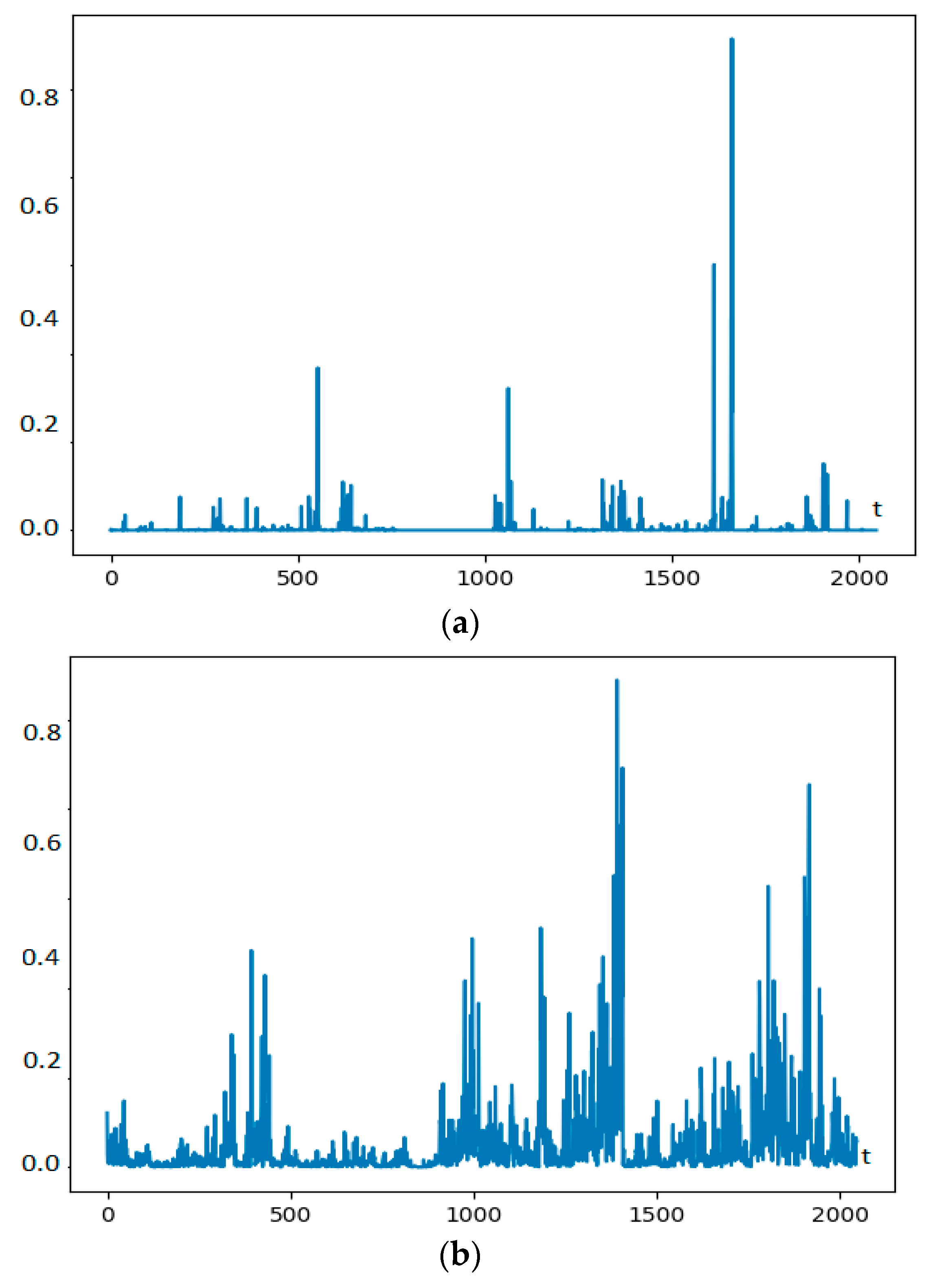
Figure 1. Multifractal cascade time series: (a) H = 0.7 ; (b) H = 0.9 .
Data 04 00005 g001
Figure 2. The result of classification: (a) training samples; (b) test samples.
Data 04 00005 g002
Figure 3. Distribution of probabilities of determining the class number, depending on the Hurst exponent value: (a) random forest; (b) direct time series estimation.
Data 04 00005 g003
Figure 4. Realizations of distributed denial-of-service (DDoS) attacks.
Data 04 00005 g004
Figure 5. Model realization of traffic that contains a DDoS attack, attack level 15%.
Data 04 00005 g005
Table 1. Standard deviations of the estimates of H depending on time series length.
N 500100020004000
S ( N ) 0.0850.070.0550.045
Table 2. Probabilities of class determination.
Time Series LengthBaggingRandom Forest
Classification TreesRegression TreesClassification TreesRegression Trees
5120.6350.7770.8110.835
10240.6440.8420.8220.882
20480.6650.8340.8340.912
40960.7010.8780.8510.922
Table 3. Average probabilities of class determination.
LengthRandom ForestTime Series Estimate H
PP
11 classes5120.720.18
40960.760.25
2 classes5120.940.75
40960.960.78
Table 4. Average probability of attack detection.
H0.51–0.60.6–0.70.7–0.80.8–0.90.9–0.99
Probability0.960.910.850.760.68