A Novel Neuro-Fuzzy Model for Multivariate Time-Series Prediction ^†

Abstract

Time series forecasting can be a complicated problem when the underlying process shows high degree of complex nonlinear behavior. In some domains, such as financial data, processing related time-series jointly can have significant benefits. This paper proposes a novel multivariate hybrid neuro-fuzzy model for forecasting tasks, which is based on and generalizes the neuro-fuzzy model with consequent layer multi-variable Gaussian units and its learning algorithm. The model is distinguished by a separate consequent block for each output, which is tuned with respect to the its output error only, but benefits from extracting additional information by processing the whole input vector including lag values of other variables. Numerical experiments show better accuracy and computational performance results than competing models and separate neuro-fuzzy models for each output, and thus an ability to implicitly handle complex cross correlation dependencies between variables.

1. Introduction

Time-series represent data points ordered in the time domain and they arise in many fields including economics, engineering, sociology, and medicine. Mathematical tools for time-series forecasting can crucially improve the decision-making process. Statistical models have dominated the field of quantitative time-series analysis for decades. These models are predominantly parametric and therefore require time-series to be weakly stationary, which is achieved through various differencing techniques, whose effectiveness is disputed [1,2] due to the highly nonstationary and nonlinear nature of real-life time-series.

The computational intelligence (CI) approach proposes nature-inspired models and methods that have been competing against classical statistical approaches in many applied domains. Among CI principal techniques, Artificial Neural Networks (ANN) are the most known and widely used. Many neural models have been applied to financial time-series forecasting [3,4,5]. Crone et al. [4] proved the ability of such networks to represent complex data patterns, including highly frequent, seasonal, and short time-series.

Fuzzy logic and fuzzy sets theory have been extended to a variety of mathematical objects by introducing a gradual degree of membership and have influenced uncertainty analysis [6,7]. Rule-based fuzzy models have been applied to various domains including stock market forecasting [8,9]. However, they have some essential drawbacks primarily caused by their dependence on expert knowledge or complex rule extraction methods.

Neuro-fuzzy systems combine the strengths of ANNs and fuzzy inference systems and have been successfully applied to a variety of problems. Their advantages are especially visible in rapidly changing domains with a high degree of uncertainty, e.g., routing guidance and planning [10,11], electric networks loading forecasting [12,13], complex logistics [14], crude oil blending [15], human resources portfolio management [16], and many others. Kar et al. [17] provided a brief review of neuro-fuzzy model applications including forecasting. The Adaptive Network Inference System (ANFIS), proposed by Jang [18] was the first successfully applied neuro-fuzzy model and the majority of the later models are based on it. Recently, neo-fuzzy systems [19,20,21], which are based on zero-order additive models, have been gaining popularity in various domains.

In the field of stock market prediction, examples of successfully applied neuro-fuzzy models include the ANFIS model with a modified Levenberg-Marquardt learning algorithm for Dhaka Stock Exchange day closing price prediction [22] and an ANFIS model based on an indirect approach and tested on Tehran Stock Exchange Indexes [23]. Rajab & Sharma [24] proposed an interpretable neuro-fuzzy approach to stock price forecasting applied to varies exchange series. Neuro-fuzzy prediction models have been combined with genetic algorithms [25], wavelet transform [26], support vector machines (SVM) [27], and recurrent connections in order to use dynamic memory [28,29]. Such combined models could show high effectiveness, but they suffer from the additional costs of extra clustering procedures, layers, and hyper-parameters.

Generally, neuro-fuzzy systems require many rules to cover complex nonlinear relations. To solve this issue for scenarios where input variables show a certain degree of interdependence and correlation, in Ebadzadeh & Salimi-Badr [30], multivariable Gaussian functions were used in a neuro-fuzzy model for efficient handling of correlated input space regions, but prediction performance was measured on a chaotic time-series, where the behavior may drastically vary from real-life data. Not much attention was paid to the data noise handling.

The aforementioned works primarily focused on a single output scenario, so developing a compact model with a memory-wise architecture and effective learning that can handle complex cross-correlation dependencies between different input times series is a necessary task. The learning procedure should combine generalization and smoothing abilities in order to work on small and noisy datasets.

In this work, we present a novel neuro-fuzzy model and a corresponding learning procedure for time-series forecasting. This model has three advantages: (1) achieves better accuracy through using the representational abilities of the multivariable Gaussian functions in the fourth layer; (2) shows good computational performance, which is achieved by using a stochastic gradient optimization procedure for tuning consequent layer units and an iterative projective algorithm for tuning their weights; and (3) has a reasonable amount of hyperparameters that can be chosen.

The remainder of this paper is organized as follows: Section 2 describes the data set that was used for numerical experiments, Section 3 is devoted to the proposed model architecture and learning, and Section 4 contains experimental results.

2. Data Description

In order to verify our model performance, we used the log returns of IBM stock and the S&P 500 index from January 1926 to December 1999 with 888 monthly records as the dataset. Correspondingly, the dataset had two columns with numerical values: IBM represents the log returns of IBM stock, and SP column contains the S&P 500 index values. These two returns comprise a bivariate concurrently correlated time series [31]. We chose this dataset as a framework due to its well-studied statistical properties and real-life nature. The original dataset can be found in Tsay [31,32] and Table 1 contains a randomly chosen block of 10 lines.

Table 1. Records example of the IBM stock and the S&P 500 index dataset.

IBM	SP
−8.24798	−4.06866
6.67236	−4.81089
4.73701	7.43094
0.70948	2.61842
3.81336	7.52652
0.00000	0.29955
−4.91377	−5.46357
8.11467	0.75415
−4.96210	−3.05211
8.11467	0.75415

Data were normalized in order to compare different models properly. Figure 1 shows the first 300 records in the normalized version of the dataset.

Figure 1. First 300 records of the normalized IBM stock and the S&P 500 index dataset.

3. Proposed Model

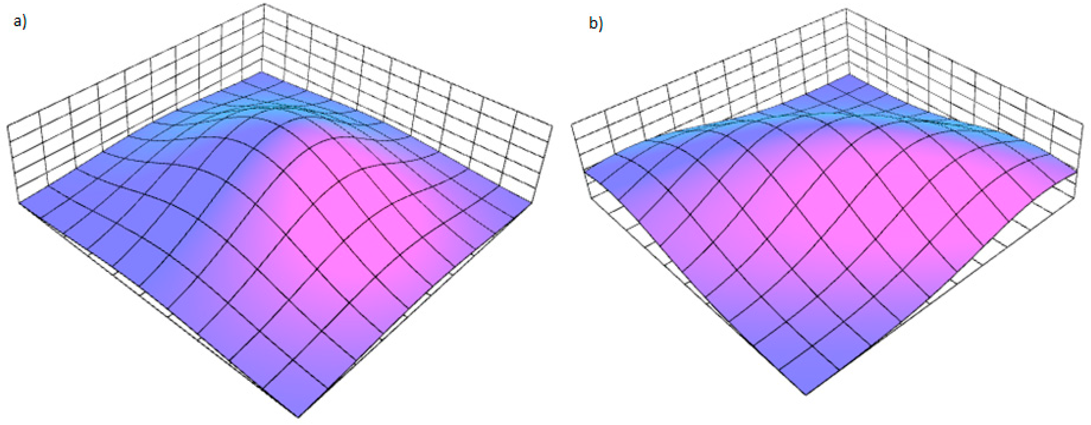
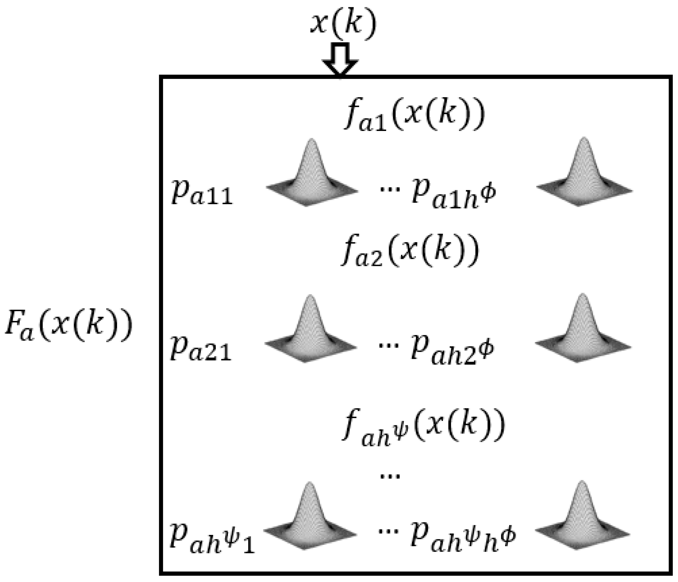
3.1. Architecture and Inference

The proposed model is a multi-output generalization of the model introduced in Vlasenko et al. [33,34], based on the classical ANFIS [18] model. It consists of five layers that are shown in the Figure 2. The main difference with the architecture described in Vlasenko et al. [33] is that we have $m$ outputs $\widehat{y}\left(k\right)={({\widehat{y}}_1(k),{\widehat{y}}_2(k),\mathrm{...},{\widehat{y}}_m(k))}^T$ instead of just one $\widehat{y}$ for each input pattern $x\left(k\right)={(x_1(k),x_2(k),\mathrm{...},x_n(k))}^T$ and, correspondingly, $m$ composite consequent layer units $F={(F_1(k),F_2(k),\mathrm{...},F_m(k))}^T$. Figure 2 depicts the modified architecture.

Figure 2. Architecture of the proposed neuro-fuzzy model.

The fuzzification layer consists of $h^{\psi }$ membership functions for each input variable; hence, their total amount is $h^{\psi }\times n$. Gaussian membership functions are used—this type of membership function is also known as a radial basis function kernel, popular among a variety of machine learning techniques. It has the following form:

$${\psi }_{jl}\left(x\left(k\right)\right)=\exp \left(-\frac{\left(x\left(k\right)-c_{jl}^{\psi }\right)}{2{{\displaystyle \sigma }}_{je}^2}\right),$$

(1)

where $x\left(k\right)$ corresponds to a current input vector, $c_{jl}^{\psi }$ is the centre, and ${\sigma }_{jl}^{}$ is a variety or width parameter, which controls the width of the bell curve.

On the initialization step, the first layer membership function centers $c_{jl}^{\psi }$ are placed at equidistant widths fixed at ${\sigma }_{jl}^{}=0.15$. An example with $h^{\psi }=5$ is shown in Figure 3.

Figure 3. Example of the first layer membership functions.

The second layer performs an aggregation of the antecedent premises. It comprises $h^{\psi }$ algebraic product fuzzy T-norm units $g$. Its outputs are computed by the formula:

$$g_j(k)={\displaystyle \prod _{i=1}^n{\psi }_{jl}\left(x_i\left(k\right)\right)}.$$

(2)

The third layer is non-parametrised and responsible for normalization. It also has $h^{\psi }$ units, which outputs calculated by the following formula:

$${\overline{g}}_j(k)=\frac{g_j(k)}{{\displaystyle \sum _{j=1}^{h^{\psi }}{g}_j(k)}}=\frac{{\displaystyle \prod _{i=1}^n{\psi }_{jl}\left(x_i\left(k\right)\right)}}{{\displaystyle \sum _{i=1}^{h^{\psi }}{\displaystyle \prod _{i=1}^n{\psi }_{jl}\left(x_i\left(k\right)\right)}}}.$$

(3)

This fulfils the Ruspini condition, which states the sum of various membership grades of one element is one [5]:

$${\displaystyle \sum _{j=1}^{h^{\psi }}{\overline{g}}_j(k)}=1.$$

(4)

The fourth layer is represented by the consequent units $F_a$ that contain multidimensional Gaussian consequent functions ${\varphi }_{aje}\left(x\left(k\right)\right)$ and weights $p_{aje}$. Multidimensional Gaussian functions replace the standard ANFIS polynomials and have the following form:

$${\varphi }_{aje}\left(x\left(k\right)\right)=\exp \left(-\frac{{\left(x\left(k\right)-c_{aje}^{\varphi }\right)}^T{Q}_{aje}^{-1}\left(x\left(k\right)-c_{aje}^{\varphi }\left(k\right)\right)}{2}\right),$$

(5)

where $x\left(k\right)$ represents an input vector, $c_{aje}^{\varphi }$ is a vector-centre of the current Gaussian, and $Q_{aje}^{}$ is the receptive field (covariance) matrix.

This function allows handling data distributed unevenly on the main axes. In case of a diagonal matrix, multidimensional Gaussian simply represents a collection of independent Gaussians with fixed width (Figure 4a).

Figure 4. The examples of multidimensional Gaussain with the same centre but different covariance matrices: (a) with diagonal matrix and (b) with matrix $\left[\begin{array}{cc}0.9& 0.6\\ 0.7& 0.9\end{array}\right]$.

The detailed structure of the consequent unit $F_a$, for each output ${\widehat{y}}_a$ is depicted in Figure 5.

Figure 5. Detailed fourth layer representation.

The consequent layer output is:

$$f_{aj}(x(k))={\displaystyle \sum _{e=1}^{h^{\varphi }}{p}_{aje}{\varphi }_{aje}\left(x\left(k\right)\right)},$$

(6)

where $h^{\varphi }$ is an amount of multidimensional Gaussian functions for each unit $f_j$.

The output layer is non-parametrized and computed as a sum of its inputs:

$${\widehat{y}}_a={\displaystyle \sum _{j=1}^{h^{\varphi }}{g}_{aj}{f}_{aj}\left(x\left(k\right)\right)}.$$

(7)

3.2. Learning Procedure

The proposed learning method generalizes the learning approach proposed by Vlasenko et al. [33] for a multivariate case. It comprises two simultaneous processes: optimization in the weights space P and in the consequent functions space.

During the initialization step, the fourth layer function centres $c_{ajl}^{\varphi }$ are placed equidistantly and $Q_{ajl}^{}$ is initialized as identity matrices. Weights $p$ are all originally set to 0.1.

Weights learning is performed by the Kachmarz method, which is a form of alternating projection method based on solving linear equation systems. It has gained popularity in signal processing, machine learning, and other domains. Each $p_a$ has the following form:

$$p_a\left(k+1\right)=p_a\left(k\right)+\frac{y_a\left(k\right)-p_a{}^T{f}_a\left(x\left(k\right)\right)}{f_a{}^T\left(x\left(k\right)\right)f_a\left(x\left(k\right)\right)}{f}_a\left(x\left(k\right)\right),$$

(8)

where $p_a\left(k\right)$ is a weights matrix, $y_a\left(k\right)$ is a reference signal, and $p_a{}^T{f}_a\left(x\left(k\right)\right)$ is the model output.

Figure 6 shows a simplified example of the error surface in the weights space.

Figure 6. Weights error surface example.

The first-order stochastic, or online in terms of machine learning theory, gradient optimization method is used for consequent functions tuning. Stochastic gradient methods have been shown to have many advantages in comparison to popular batch gradient methods in real-life optimization problems including machine learning applications [35,36]. Instead of computing the full gradient over all dataset in batches, these methods update free model parameters after processing each input pattern. Their main advantage is the inherent noise of calculated gradients. Additionally, they do not suffer from rounding errors, which occur when having to store the accumulated gradient [37], and have better computational performance. The disadvantage is that they cannot be as easily parallelized as batch methods [36,37] and the severity of such restriction depends on the domain.

Learning is based on the standard mean square error criterion:

$$E=\frac{1}{N}{\displaystyle \sum _{k=1}^N{(y(k)-\widehat{y}(k))}^2},$$

(9)

where $y\left(k\right)$ is the reference signal value, $\widehat{y}(k)$ is the prognosis signal value, and $N$ is the training set length.

The centres $c_{ajl}^{\varphi }$ are then tuned using:

$$\{\begin{array}{c}{c}_{ajl}^{\varphi }\left(k+1\right)=c_{ajl}^{\varphi }\left(k\right)+{\lambda }_c\frac{{\tau }_{ajl}^c\left(k\right)e\left(k\right)}{{\eta }_c\left(k\right)}\\ {\eta }_{ac}\left(k+1\right)={\beta }_c{\eta }_{ac}\left(k\right)+{\tau }_{ajl}^c{}^T{\tau }_{ajl}^c\end{array},$$

(10)

where ${\lambda }_c$ is a learning step, ${\beta }_c$ is a dumping parameter, and ${\tau }_{ajl}^c$ is a vector of back propagated gradient values with respect to $c_{ajl}^{\varphi }$.

The $Q_{ajl}^{}$ matrices learning can be written as:

$$\{\begin{array}{c}{Q}_{ajl}\left(k+1\right)=Q_{ajl}\left(k\right)+{\lambda }_Q\frac{{\tau }_{ajl}^Q\left(k\right)e\left(k\right)}{{\eta }_{aq}\left(k\right)}\hfill \\ {\eta }_{aQ}\left(k+1\right)={\beta }_Q{\eta }_{aQ}\left(k\right)+Tr\left({\tau }_{ajl}^Q{}^T{\tau }_{ajl}^Q\right)\hfill \end{array},$$

(11)

where ${\lambda }_Q$ is a learning step, ${\beta }_Q$ is a dumping parameter, and ${\tau }_{ajl}^Q$ is a matrix of values back propagated with respect to $Q_{ajl}^{}$.

Vectors ${\eta }_{ac}$ and matrices ${\eta }_{aQ}$ represent the decaying average value of past gradients and the algorithm initializes with ${\eta }_{ac}={\eta }_{aQ}=10,000$.

Figure 7 depicts an example of the error surface with respect to centres $c_{ajl}^{\varphi }$ and Figure 8 shows examples of multidimensional Gaussians after learning is finished.

Figure 7. An example of the error function surface in a simplified two-dimensional case.

Figure 8. Examples of the two-dimensional Gaussian functions after learning.

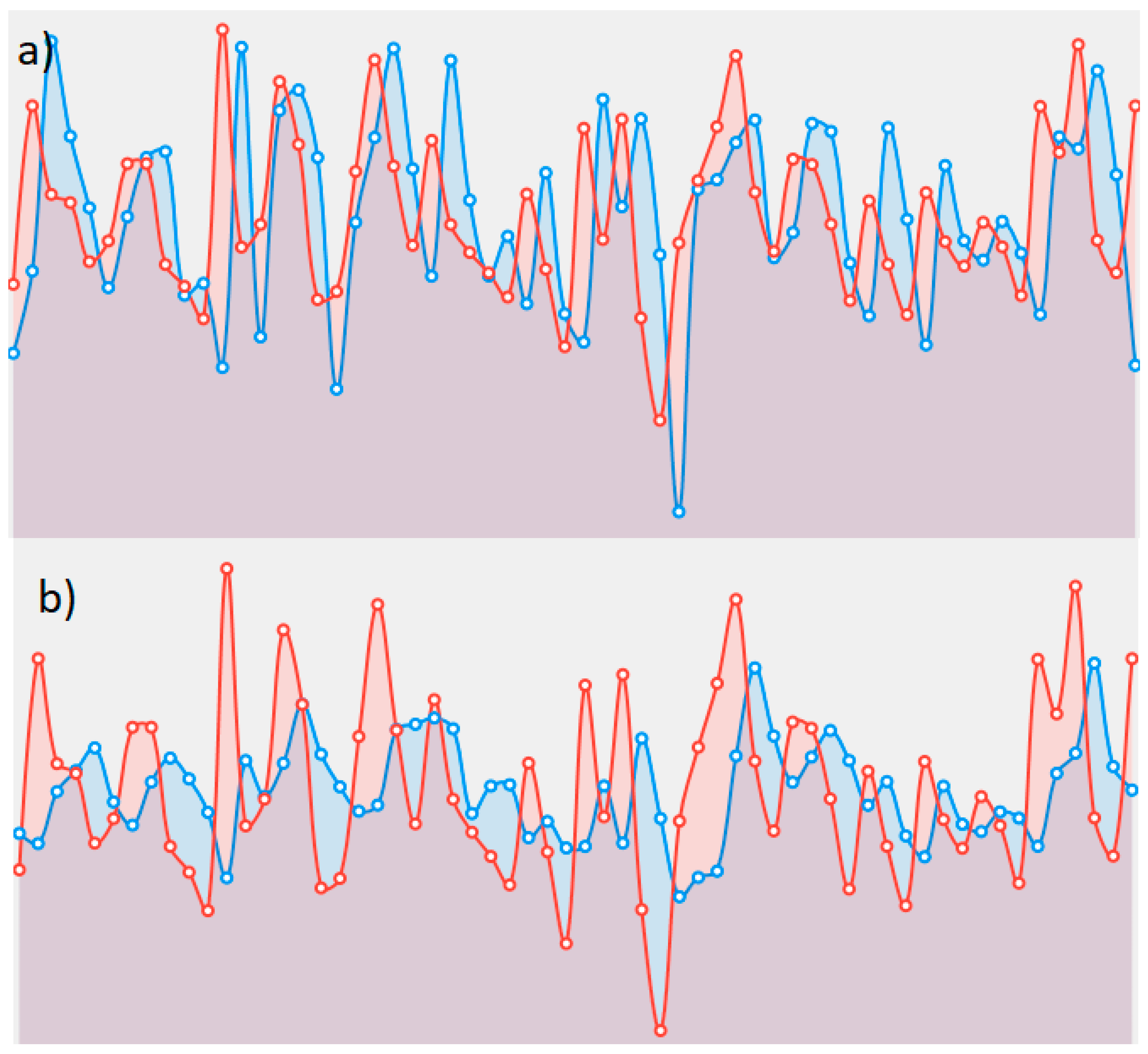
4. Experimental Results

We compared the prediction accuracy and computational performance to ANN using bipolar sigmoid activation functions. To train the ANN model, we used the Levenberg-Marquardt algorithm [38] and resilient backpropagation learning algorithm (RPROP) [39] as the popular batch optimization techniques.

The Accord.NET package [40] was used for the ANN implementations and we wrote custom software for the neuro-fuzzy model. In addition, we utilized the Math.NET Numerics package [41] for the linear algebra operations in the neuro-fuzzy model implementation.

The experiments were performed on a computer with Intel ^® Core(TM) Core i7-7700 processor (Intel, Santa Clara, California, U.S.) and 32 GB of memory.

Root Mean Square Error (RMSE) and Symmetric Mean Absolute Percent Error (SMAPE) criteria were used to estimate prediction accuracy:

$$RMSE=\sqrt{\frac{{\displaystyle \sum _{k=1}^N{(y(k)-\widehat{y}(k))}^2}}{N}},$$

$$SMAPE=\frac{2}{N}{\displaystyle \sum _{k=1}^N\frac{\left|\widehat{y}(k)-y(k)\right|}{\widehat{y}(k)+y(k)}},$$

where $y\left(k\right)$ is a reference signal value, $\widehat{y}(k)$ is a prognosis signal value, and $N$ is the training set length.

The bipolar sigmoid networks were built from sigmoids with an alpha value 0.4 for all cases, learning rate 0.67, and 50 epochs were used for resilient backpropagation. The Levenberg-Marquardt implementation was trained with 10 epochs. The neuro-fuzzy model had the following parameters $h^{\psi }=3$, ${\lambda }_c=1$, and ${\lambda }_Q=1$.

The original dataset was divided into a training set of 660 records and 228 records in the validation set. The input vectors for the bivariate case were composed of an equal number of sequential numbers from both dataset components.

We also compared the performance of all models in a univariate case, which is reflected in Table 2.

Table 2. Experimental results.

Model	IBM Stock Daily Log Returns and S&P 500 Index Dataset Results
	Execution time (ms)	IBM stock RMSE (%)	IBM stock SMAPE (%)	S&P 500 index RMSE (%)	S&P 500 index SMAPE (%)
Proposed model $h^{\varphi }=1,{\beta }_c=0.89,{\beta }_Q=0.98$	64	8.938	10.049	4.443	4.594
$h^{\varphi }=1,{\beta }_c=1.19,{\beta }_Q=0.97$	39	12.956	20.548	-	-
$h^{\varphi }=1,{\beta }_c=0.88,{\beta }_Q=0.93$	38	-	-	6.097	9.005
Proposed model $h^{\varphi }=2,{\beta }_c=0.85,{\beta }_Q=0.93$	120	8.878	10.104	4.356	4.532
$h^{\varphi }=2,{\beta }_c=0.82,{\beta }_Q=0.91$	63	12.865	20.138	-	-
$h^{\varphi }=2,{\beta }_c=0.75,{\beta }_Q=0.92$	65	-	-	6.056	8.677
Proposed model $h^{\varphi }=4,{\beta }_c=0.78,{\beta }_Q=0.91$	257	8.866	10.013	4.294	4.463
$h^{\varphi }=4,{\beta }_c=0.75,{\beta }_Q=0.91$	126	12.693	20.133	-	-
$h^{\varphi }=4,{\beta }_c=0.74,{\beta }_Q=0.93$	110	-	-	6.113	8.775
Bipolar Sigmoid Network RBPR	847	8.91	10.156	4.66	4.96
	514	13.162	20.876
	545	-	-	6.308	9.139
Bipolar Sigmoid Network Levenberg-Marquart	302	8.940	10.07	4.542	4.755
	313	14.544	22.664	-	-
	297	-	-	7.025	11.019

The performed experiments showed that ANN with a resilient backpropagation needs a significant number of epochs to attain good accuracy, greatly reducing computational performance. Levenberg-Marquardt learning requires fewer epochs, but each epoch costs more in terms of computing.

The proposed model demonstrated better performance results in all cases—both computational time and accuracy were significantly better than those of competitors. Also, the results in Table 2 show that accuracy improves with a larger $h^{\varphi }$, but the downside is longer execution time.

The multivariate neuro-fuzzy model requires less computational resources than the two independent univariate models and has drastically better accuracy.

Visualization of the learning process is presented in Figure 9 and Figure 10; IBM stock returns are depicted for the multivariate and univariate cases. Figure 9 shows the significant improvement in the forecasting plot obtained using the multivariate neuro-fuzzy model. Conversely, Figure 10 does not show such a degree of improvement for the bipolar sigmoid artificial neural model.

Figure 9. Learning process plot for the proposed neuro-fuzzy model: red dots—IBM stock returns actual values, blue—predicted values. (a) bivariate model; (b) univariate model.

Figure 10. Learning process plot for bipolar sigmoid artificial neural model with resilient backpropagation learning: red dots—IBM stock returns actual values, blue—predicted values. (a) bivariate model; (b) univariate model.

5. Conclusions

In this paper, we introduced a novel multiple output neuro-fuzzy model with multidimensional Gaussian functions in the consequent layer. The proposed model expands upon existing single output neuro-fuzzy models by adding separate fourth layer composed of computational units for each output. The model allows optimal training performance with respect to other outputs by implicitly handling lagged cross-correlation relations, which are common in financial data.

Experimental simulations demonstrated the good computational performance and prediction accuracy of our model in comparison to well-known ANN models. In addition, the advantage of utilizing multivariate time-series was proven.

References

- Commandeur, J.J.; Koopman, S.J. An Introduction to State Space Time Series Analysis; Oxford University Press: Oxford, UK, 2007. [Google Scholar]
- Logue, A.C. The Efficient Market Hypothesis and Its Critics. CFA Digest 2003, 33, 40–41. [Google Scholar] [CrossRef]
- Weigend, A.S.; Huberman, B.A.; Rumelhart, D.E. Predicting the future: A connectionist approach. Int. J. Neural Syst. 1990, 1, 193–209. [Google Scholar] [CrossRef]
- Crone, S.F.; Hibon, M.; Nikolopoulos, K. Advances in forecasting with neural networks? Empirical evidence from the NN3 competition on time series prediction. Int. J. Forecast. 2011, 27, 635–660. [Google Scholar] [CrossRef]
- Bodyanskiy, Y.; Popov, S. Neural network approach to forecasting of quasiperiodic financial time series. Eur. J. Oper. Res. 2006, 175, 1357–1366. [Google Scholar] [CrossRef]
- Dubois, D.; Prade, H. The legacy of 50 years of fuzzy sets: A discussion. Fuzzy Sets Syst. 2015, 281, 21–31. [Google Scholar] [CrossRef]
- Dubois, D.; Prade, H. Gradualness, uncertainty and bipolarity: Making sense of fuzzy sets. Fuzzy Sets Syst. 2012, 192, 3–24. [Google Scholar] [CrossRef]
- Sheta, A. Software Effort Estimation and Stock Market Prediction Using Takagi-Sugeno Fuzzy Models. In Proceedings of the 2006 IEEE International Conference on Fuzzy Systems, Vancouver, BC, Canada, 16–21 July 2006. [Google Scholar] [CrossRef]
- Chang, P.-C.; Liu, C.-H. A TSK type fuzzy rule based system for stock price prediction. Expert Syst. Appl. 2008, 34, 135–144. [Google Scholar] [CrossRef]
- Pamučar, D.; Cirovic, G. Vehicle Route Selection with an Adaptive Neuro Fuzzy Inference System in Uncertainty Conditions. Decis. Mak. Appl. Manag. Eng. 2018, 1, 13–37. [Google Scholar] [CrossRef]
- Pamučar, D.; Ljubojević, S.; Kostadinović, D.; Đorović, B. Cost and risk aggregation in multi-objective route planning for hazardous materials transportation—A neuro-fuzzy and artificial bee colony approach. Expert Syst. Appl. 2016, 65, 1–15. [Google Scholar] [CrossRef]
- Bodyanskiy, Y.; Popov, S.; Rybalchenko, T. Multilayer Neuro-fuzzy Network for Short Term Electric Load Forecasting. In Lecture Notes in Computer Science; Springer: Berlin/Heidelberg, Germany, 2008; pp. 339–348. [Google Scholar]
- Otto, P.; Bodyanskiy, Y.; Kolodyazhniy, V. A new learning algorithm for a forecasting neuro-fuzzy network. Integr. Comput.-Aided Eng. 2003, 10, 399–409. [Google Scholar] [CrossRef]
- Sremac, S.; Tanackov, I.; Kopić, M.; Radović, D. ANFIS model for determining the economic order quantity. Decis. Mak. Appl. Manag. Eng. 2018, 1. [Google Scholar] [CrossRef]
- De Jesús Rubio, J. USNFIS: Uniform stable neuro fuzzy inference system. Neurocomputing 2017, 262, 57–66. [Google Scholar] [CrossRef]
- Lukovac, V.; Pamučar, D.; Popović, M.; Đorović, B. Portfolio model for analyzing human resources: An approach based on neuro-fuzzy modeling and the simulated annealing algorithm. Expert Syst. Appl. 2017, 90, 318–331. [Google Scholar] [CrossRef]
- Kar, S.; Das, S.; Ghosh, P.K. Applications of neuro fuzzy systems: A brief review and future outline. Appl. Soft Comput. 2014, 15, 243–259. [Google Scholar] [CrossRef]
- Jang, J.S. ANFIS: Adaptive-network-based fuzzy inference system. IEEE Trans. Syst. Man Cybern. 1993, 23, 665–685. [Google Scholar] [CrossRef]
- Mendes, J.; Souza, F.; Araújo, R.; Rastegar, S. Neo-fuzzy neuron learning using backfitting algorithm. Neural Comput. Appl. 2017. [Google Scholar] [CrossRef]
- Silva, A.M.; Caminhas, W.; Lemos, A.; Gomide, F. A fast learning algorithm for evolving neo-fuzzy neuron. Appl. Soft Comput. 2014, 14, 194–209. [Google Scholar] [CrossRef]
- Bodyanskiy, Y.V.; Tyshchenko, O.K.; Kopaliani, D.S. Adaptive learning of an evolving cascade neo-fuzzy system in data stream mining tasks. Evol. Syst. 2016, 7, 107–116. [Google Scholar] [CrossRef]
- Billah, M.; Waheed, S.; Hanifa, A. Stock market prediction using an improved training algorithm of neural network. In Proceedings of the 2nd International Conference on Electrical, Computer & Telecommunication Engineering (ICECTE), Rajshahi, Bangladesh, 8–10 December 2016. [Google Scholar] [CrossRef]
- Esfahanipour, A.; Aghamiri, W. Adapted Neuro-Fuzzy Inference System on indirect approach TSK fuzzy rule base for stock market analysis. Expert Syst. Appl. 2010, 37, 4742–4748. [Google Scholar] [CrossRef]
- Rajab, S.; Sharma, V. An interpretable neuro-fuzzy approach to stock price forecasting. Soft Comput. 2017. [Google Scholar] [CrossRef]
- Hadavandi, E.; Shavandi, H.; Ghanbari, A. Integration of genetic fuzzy systems and artificial neural networks for stock price forecasting. Knowl.-Based Syst. 2010, 23, 800–808. [Google Scholar] [CrossRef]
- Bodyanskiy, Y.; Pliss, I.; Vynokurova, O. Adaptive wavelet-neuro-fuzzy network in the forecasting and emulation tasks. Int. J. Inf. Theory Appl. 2008, 15, 47–55. [Google Scholar]
- Chiu, D.-Y.; Chen, P.-J. Dynamically exploring internal mechanism of stock market by fuzzy-based support vector machines with high dimension input space and genetic algorithm. Expert Syst. Appl. 2009, 36, 1240–1248. [Google Scholar] [CrossRef]
- Parida, A.K.; Bisoi, R.; Dash, P.K.; Mishra, S. Times Series Forecasting using Chebyshev Functions based Locally Recurrent neuro-Fuzzy Information System. Int. J. Comput. Intell. Syst. 2017, 10, 375. [Google Scholar] [CrossRef]
- Atsalakis, G.S.; Valavanis, K.P. Forecasting stock market short-term trends using a neuro-fuzzy based methodology. Expert Syst. Appl. 2009, 36, 10696–10707. [Google Scholar] [CrossRef]
- Ebadzadeh, M.M.; Salimi-Badr, A. CFNN: Correlated fuzzy neural network. Neurocomputing 2015, 148, 430–444. [Google Scholar] [CrossRef]
- Tsay, R.S. Analysis of Financial Time Series; Wiley Series in Probability and Statistics; John Wiley & Sons: Hoboken, NJ, USA, 2005. [Google Scholar] [CrossRef]
- Monthly Log Returns of IBM Stock and the S&P 500 Index Dataset. Available online: https://faculty.chicagobooth.edu/ruey.tsay/teaching/fts/m-ibmspln.dat (accessed on 1 September 2018).
- Vlasenko, A.; Vynokurova, O.; Vlasenko, N.; Peleshko, M. A Hybrid Neuro-Fuzzy Model for Stock Market Time-Series Prediction. In Proceedings of the IEEE Second International Conference on Data Stream Mining & Processing (DSMP), Lviv, Ukraine, 21–25 August 2018. [Google Scholar] [CrossRef]
- Vlasenko, A.; Vlasenko, N.; Vynokurova, O.; Bodyanskiy, Y. An Enhancement of a Learning Procedure in Neuro-Fuzzy Model. In Proceedings of the IEEE First International Conference on System Analysis & Intelligent Computing (SAIC), Kyiv, Ukraine, 8–12 October 2018. [Google Scholar] [CrossRef]
- LeCun, Y.A.; Bottou, L.; Orr, G.B.; Müller, K.-R. Efficient BackProp. Neural Netw. Tricks Trade 2012, 9–48. [Google Scholar] [CrossRef]
- Bottou, L.; Curtis, F.E.; Nocedal, J. Optimization Methods for Large-Scale Machine Learning. SIAM Rev. 2018, 60, 223–311. [Google Scholar] [CrossRef]
- Wiesler, S.; Richard, A.; Schluter, R.; Ney, H. A critical evaluation of stochastic algorithms for convex optimization. In Proceedings of the IEEE International Conference on Acoustics, Speech and Signal Processing, Vancouver, BC, Canada, 26–30 May 2013. [Google Scholar] [CrossRef]
- Kanzow, C.; Yamashita, N.; Fukushima, M. Erratum to “Levenberg–Marquardt methods with strong local convergence properties for solving nonlinear equations with convex constraints. J. Comput. Appl. Math. 2005, 177, 241. [Google Scholar] [CrossRef]
- Riedmiller, M.; Braun, H. A direct adaptive method for faster backpropagation learning: The RPROP algorithm. In Proceedings of the IEEE International Conference on Neural Networks, Rio, Brazil, 8–13 July 2018. [Google Scholar] [CrossRef]
- Souza, C.R. The Accord.NET Framework. Available online: http://accord-framework.net (accessed on 1 November 2018).
- Math.NET Numerics. Available online: https://numerics.mathdotnet.com (accessed on 1 November 2018).
© 2018 by the authors. Licensee MDPI, Basel, Switzerland. This article is an open access article distributed under the terms and conditions of the Creative Commons Attribution (CC BY) license (http://creativecommons.org/licenses/by/4.0/).