Article

Applications of Machine Learning for Wine Recognition Based on 1H-NMR Spectroscopy

by
Ariana Raluca Hategan
1,2,
Adrian Pirnau
1 and
Dana Alina Magdas
1,2,*
1
National Institute for Research and Development of Isotopic and Molecular Technologies, 67-103 Donat Street, 400293 Cluj-Napoca, Romania
2
Faculty of Physics, Babeș-Bolyai University, Kogălniceanu 1, 400084 Cluj-Napoca, Romania
*
Author to whom correspondence should be addressed.
Beverages 2025, 11(2), 45; https://doi.org/10.3390/beverages11020045
Submission received: 23 January 2025 / Revised: 11 March 2025 / Accepted: 24 March 2025 / Published: 27 March 2025

Abstract

:
The present study aims to explore the possibility of applying machine learning (ML) algorithms for the development of reliable wine authentication instruments able to encompass the exhaustive performances offered by learning-based methods, and, at the same time, to propose reference practices for improving the recognition ability of the developed models. In this regard, two ML algorithms, namely k-Nearest Neighbors (kNN) and Logistic Regression, have been utilized as supervised learning techniques applied to 1H-NMR spectral data for the development of classification models able to recognize the variety, geographical origin, and vintage of wine samples. Due to the complexity of the experimental data, which was characterized by a high number of variables, special attention was given to the preprocessing phase in order to identify the most relevant input space for each envisaged classification criterion. The obtained results have shown that 1H-NMR spectroscopy in conjunction with Logistic Regression represents a reliable approach for wine traceability, leading, for all investigated classification criteria, to accuracy scores of the developed models greater than 98% in cross-validation and up to 100% in testing.

1. Introduction

Food and beverage authenticity controls represent a continuous preoccupation for all involved actors, from authorities to consumers. Among all commodities, wine is one of the top ten most often adulterated products [1,2]. On average, wine consists of 86% water, 11% ethanol, and various other compounds such as sugars, phenols, mineral or organic acids (e.g., fumaric, malic, and succinic acid) [3]. The most common forms of wine falsification are represented, among others, by the false declaration of the geographical origin, cultivar, or vintage [4,5]. Therefore, enormous efforts were made in the development of reliable analytical approaches able to detect these types of frauds that not only have economic implications but also could be reflected in human health, too. For wines, in addition to the already acknowledged methods for control like isotope ratio mass spectrometry (IRMS) [6], new analytical approaches, classified as metabolomics or AI-based omics, based on several spectroscopic techniques like vibrational (IR, Raman/SERS) [7,8,9,10], 1H-NMR [11,12,13], or fluorescence [14,15], in corroboration with supervised statistical methods or machine learning (ML), were successfully applied [16]. Nevertheless, among all the previously mentioned techniques, for wine authentication, NMR techniques are unanimously recognized [2]. NMR spectroscopy involves the quantum magnetic properties of atomic nuclei. These properties are influenced by molecular proximity, their measurement providing a map of interatomic bonds, and a description of molecular dynamics [17]. Among the NMR techniques, 1H-NMR spectroscopy is increasingly used in the analysis of food matrices, being a non-destructive, selective method, capable of simultaneously detecting a large number of low-molecular-weight components present in a complex matrix such as wine during one single run [18,19]. Furthermore, the 1H-NMR technique is sensitive, reliable, and remarkably reproducible, having a wide linearity range. It not only allows the simultaneous quantification of an important number of metabolites but it can also fingerprint a specific pattern of a certain sample. Therefore, through a single measurement, it is possible to obtain both quantitative and qualitative information about a sample. Last but not least, a notable advantage of this technique is that NMR equipment is very robust, being almost free of maintenance. These are the most important reasons why many research groups performed considerable efforts to develop new analytical protocols for the successful application of this technique in wine differentiation [2].
The assessment of 1H-NMR data corresponds to a very challenging task, due to the complexity of the spectra or overlapping peaks. In this light, advanced data processing techniques are needed to integrate and analyze large amounts of spectral data [20]. While classic chemometric tools have their own strengths and applications for this task, ML-based approaches offer enhanced flexibility, having the ability to handle complex, nonlinear relationships. In broad terms, ML represents an important field of Artificial Intelligence (AI) related to the development of computer systems capable of automatically improving themselves through experience [21,22]. It can be regarded as the confluence of statistics and computer science, considered one of the technical areas with the fastest growth rates in the world today [22]. Such algorithms provide a powerful tool for interpreting and extracting meaningful information from NMR spectra [23], particularly in scenarios where traditional methods may fall short.
Apart from the obtainment of reliable experimental data and the application of advanced data processing techniques, an important step in the development of reliable wine differentiation models is represented by spectra pretreatment [24]. Therefore, previous reports in the literature [25] highlight the importance of the preprocessing step that needs to be applied to the experimental 1H-NMR honey spectra to improve the performance of the recognition models. It was proved that pretreating the raw data through autoscaling, variance scaling, or class centroid centering and scaling, followed by a data dimensionality reduction step, can drastically improve the capability of the developed differentiation models [25].
Against this background, the main aim of the present preliminary work is to develop reliable learning-based models for wine differentiation with respect to the geographical origin, vintage, and variety. For this purpose, two ML algorithms, namely k-Nearest Neighbors (kNN) and Logistic Regression, have been applied and subsequently compared. Special attention was given to the preprocessing phase in order to identify the input data that are the most suitable concerning each classification criterion.

2. Materials and Methods

2.1. Data Set

In total, 65 Romanian white wine samples, with the following cultivar distribution (Sauvignon Blanc—23, Chardonnay—13, Pinot Gris—9, and Riesling—20) were employed in this study. The samples were produced in three of the most famous viticultural areas of Romania, namely Transylvania (20), Moldova (22), and Muntenia (23). According to the production year, the distribution of the investigated wine samples was as follows: 2012 (15 samples), 2013 (13 samples), 2014 (15 samples), 2015 (11 samples), and 2016 (11 samples). The sample set was split into two distinct groups, a training data set consisting of 60 samples utilized for model development and optimization, and an independent external validation data set of 5 wine samples reserved for assessing the models’ performance (Table S1).

2.2. 1H-NMR Spectra Acquisition

The sample preparation protocol consisted of diluting a quantity of 900 μL of wine with 100 μL of buffered D2O solution obtained from 1 M potassium dihydrogen phosphate (99% KH2PO4, Sigma Aldrich, Schnelldorf, Germany), 3 mM sodium azide (extra pure, NaN3, Sigma Aldrich, Schnelldorf, Germany), and 0.1% 3-(trimethyl-silyl)-propionic acid sodium salt (TSP, Eurisotop, Saint - Aubin, France). Subsequently, 600 μL of this prepared sample was transferred to an NMR tube (5 mm) for 1H-NMR measurements.
The 1H-NMR determinations were made using a BRUKER Avance III 500 UltraShield NMR spectrometer operating at 500.13 MHz for protons, coupled with a 5 mm BBO (Broad Band Observe) probehead. The determinations were performed at 300 ± 0.1 K in buffered D2O solution, and the chemical shifts were measured relative to TSP (3-(trimethyl-silyl)-propionic acid sodium salt), using a standard presaturation method for suppressing the water signal. All spectra acquisition and processing steps were carried out using the TopSpin 2.1 software [26]. Typical conditions were as follows: a 64 K data point, a sweep width of 9000 Hz (18 ppm) collected 64 scans, 10.1 μs for a 90° pulse width, a 3.63 s acquisition time, and a 6 s relaxation delay.

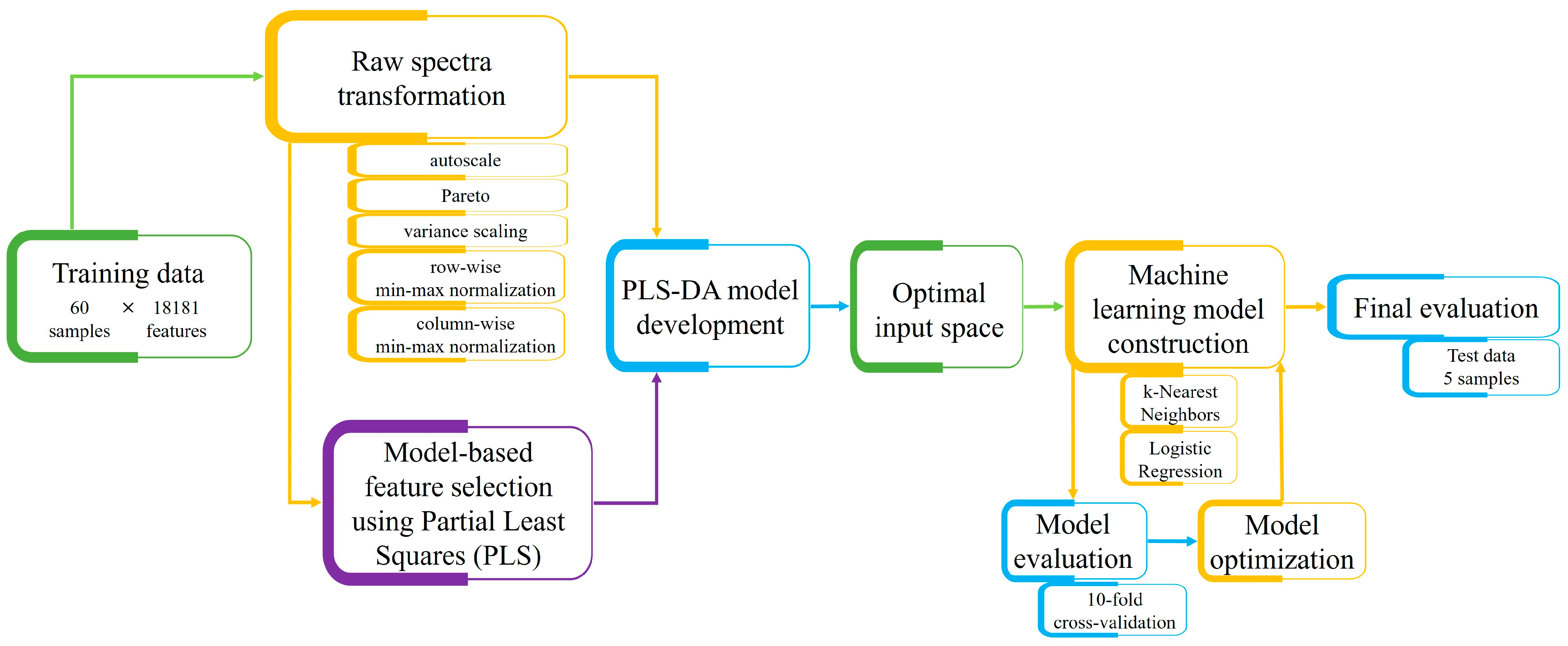
2.3. Experimental Data Preprocessing

With the aim of optimizing the input data for the development of the machine learning models, several preprocessing steps were conducted and further compared. The investigated preprocessing techniques included the application of several methods (i.e., autoscaling, variance scaling, Pareto scaling, and min–max scaling along rows and columns) for transforming the raw 1H-NMR spectra, and the reduction in the dimensionality of the data space through a model-based variable selection method that uses Partial Least Squares (PLS) regression. The potential given by the application of each preprocessing method was evaluated through the mean accuracy score determined by means of 10-fold cross-validation when Partial Least Squares Discriminant Analysis (PLS-DA) models were constructed. All data preprocessing investigations were conducted utilizing the software SOLO 8.9.1 (2021) (Eigenvector Research Inc., 2022 Manson, WA, USA, 98831).

2.3.1. Raw Spectra Transformation Techniques

Five preprocessing techniques were applied to the raw 1H-NMR spectra, namely autoscale, Pareto, variance scaling, and min–max scaling, which was utilized in two manners, once along the rows and another time on the columns of the data set, leading to different transformations of the original data. In the current work, each 1H-NMR spectrum corresponded to a single row, and the intensity of the signals of all samples at a specific ppm was associated with a column of the data matrix. By applying the autoscale method, each column was transformed such that it had a zero mean and a standard deviation of one. This was achieved by subtracting, from a column, the mean intensity value of the samples at the corresponding ppm followed by a division to the standard deviation of that column. Variance scaling and Pareto also represent preprocessing techniques that are oriented on each variable (i.e., column) of the data set and imply dividing each column by its standard deviation and by the square root of its standard deviation, respectively. Lastly, min–max scaling consists of subtracting the minimum value from a row (or column) and subsequently dividing it by the difference between the maximum and minimum associated with that row (or column). Based on these theoretical considerations, four of the applied preprocessing methods corresponded to variable-oriented techniques, whereas only one of them was applied to each data instance (i.e., spectrum-oriented) [27].

2.3.2. Data Dimensionality Reduction

To identify the spectral points with the highest discrimination power, a model-based feature selection algorithm based on Partial Least Squares (PLS) was conducted. This technique implies an iterative removal from the input space of the variables that have the lowest VIP (Variable Importance in Projection) and SR (Selectivity Ratio) scores with respect to the PLS models constructed for a specific differentiation criterion [28]. Through this approach, the 1H-NMR spectra variables that correspond to the highest differentiation power in relation to each classification criterion (i.e., cultivar, vintage, or geographical origin) were able to be determined and further used for developing the prediction models.

2.4. Machine Learning-Based Analysis

For implementing the wine discrimination models, two machine learning algorithms have been applied, namely k-Nearest Neighbors (kNN) and Logistic Regression. Due to the fact that the purpose of the present work corresponds to the development of predictive models by taking into account the training data (i.e., the recorded 1H-NMR spectra and their associated labels), these two learning techniques have been employed in the context of supervised learning.

2.4.1. K-Nearest Neighbors

K-Nearest Neighbors (kNN) can be regarded as an instance-based learning method, as it does not aim to build a general model for approximating a given target function, and instead simply stores the data associated with the training examples [22]. In the case of classification problems, the prediction of an unknown instance is determined through a straightforward majority vote of the training objects that are closest to it. In this manner, a test object is allocated to the class having the highest representation among its nearest neighbors [29]. The kNN models were developed through the use of the sklearn.neighbors.KNeighborsClassifier class [29] and were optimized by testing distinct numbers of neighbors (i.e., 1, 3, …, 15), distance functions (i.e., Euclidean and Manhattan), or weight functions (i.e., uniform and distance).

2.4.2. Logistic Regression

Logistic Regression represents a method for modeling the relationship between a binary dependent variable and several independent variables. The key idea behind Logistic Regression is to map the linear combination of the independent variables to the probability of the event occurring using a logistic function [30]. In the frame of the present study, Logistic Regression models were implemented through the use of the linear_model.LogisticRegression class available in the Python library scikit-learn (version 1.2.2). In this context, special attention was given to setting the solver (i.e., the algorithm used to optimize the model’s parameters), the penalty (i.e., the term which helps prevent overfitting through the addition of a regularization term to the loss function), the regularization parameter C, and the number of iterations [29]. This implied the use of a grid-search approach to experiment and select the combination that yields the best results for a given classification type.

2.4.3. Performance Evaluation

During the optimization stage, the performances of the learning-based models have been evaluated and compared by means of cross-validation, having the number of folds set to 10. An important aspect refers to the fact that each of the testing folds has been chosen to maintain the original distribution of the samples with respect to the investigated classes. Nonetheless, for consistency reasons, the same groups of testing instances have been used to assess the performance of each type of classifier (i.e., k-Nearest Neighbors or Logistic Regression models). This was achieved through the use of the class sklearn.model_selection.StratifiedKFold [29], having the parameter shuffle set to True and random_state set to 1. Subsequently, after the identification of the optimal hyperparameters, the machine learning models were retrained based on an entire training data set and nonetheless evaluated in regard to the test instances, ensuring an unbiased assessment of their performance.

3. Results and Discussion

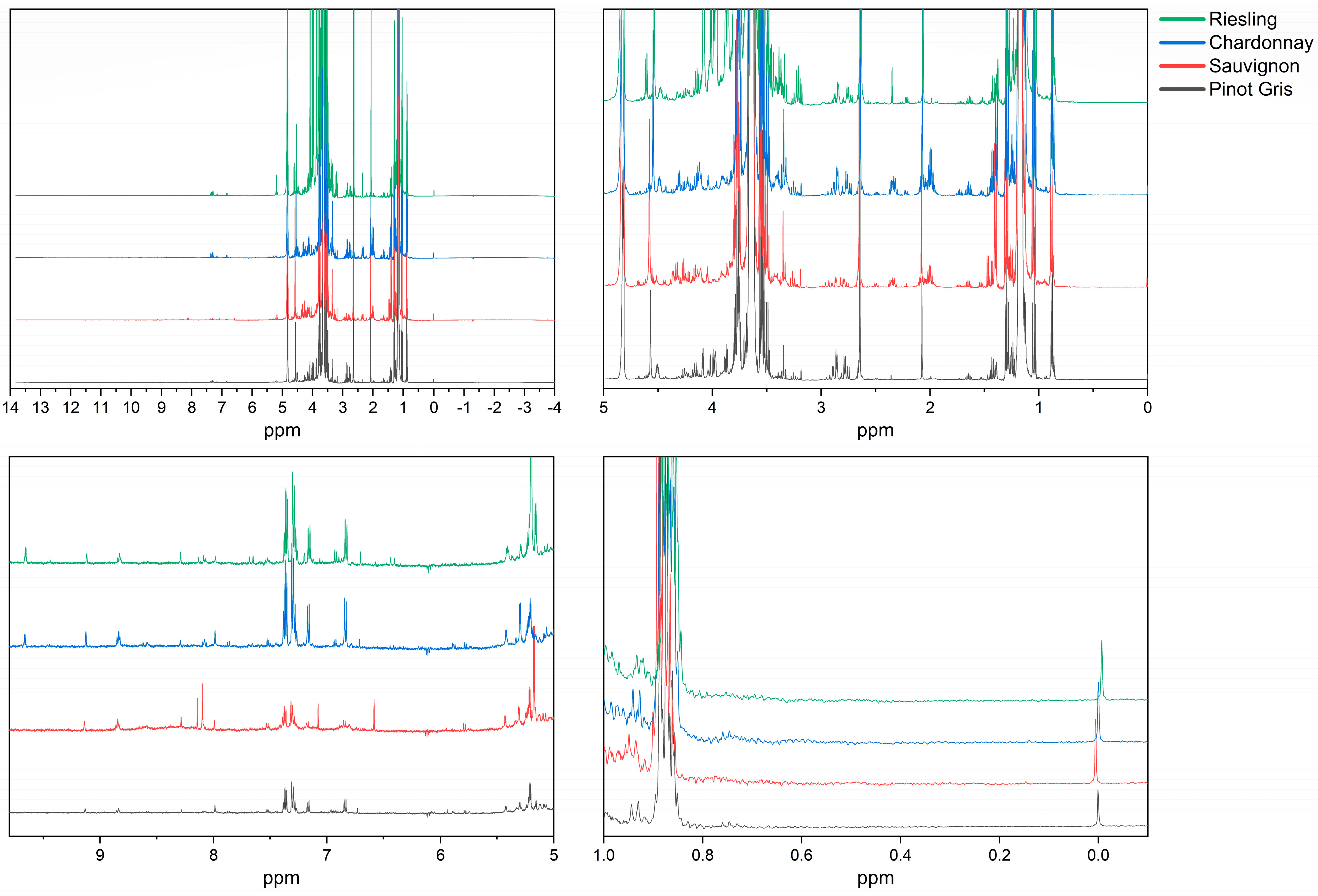
3.1. Experimental Spectra

The raw 1H-NMR measurements of the investigated wine samples were characterized by 32,768 spectral variables situated in the range of –4–14 ppm. However, due to the fact that the marginal regions of the spectra did not present any significant peaks, the spectral range that was considered for model development was between 0 and 10 ppm, comprising a total of 18,181 spectral points. As can be seen in Figure 1, this spectral region contains the peaks that correspond to the protons from ethanol, as well as protons from minor components that can be used to detect subtle differences among wine samples according to distinct classification criteria.

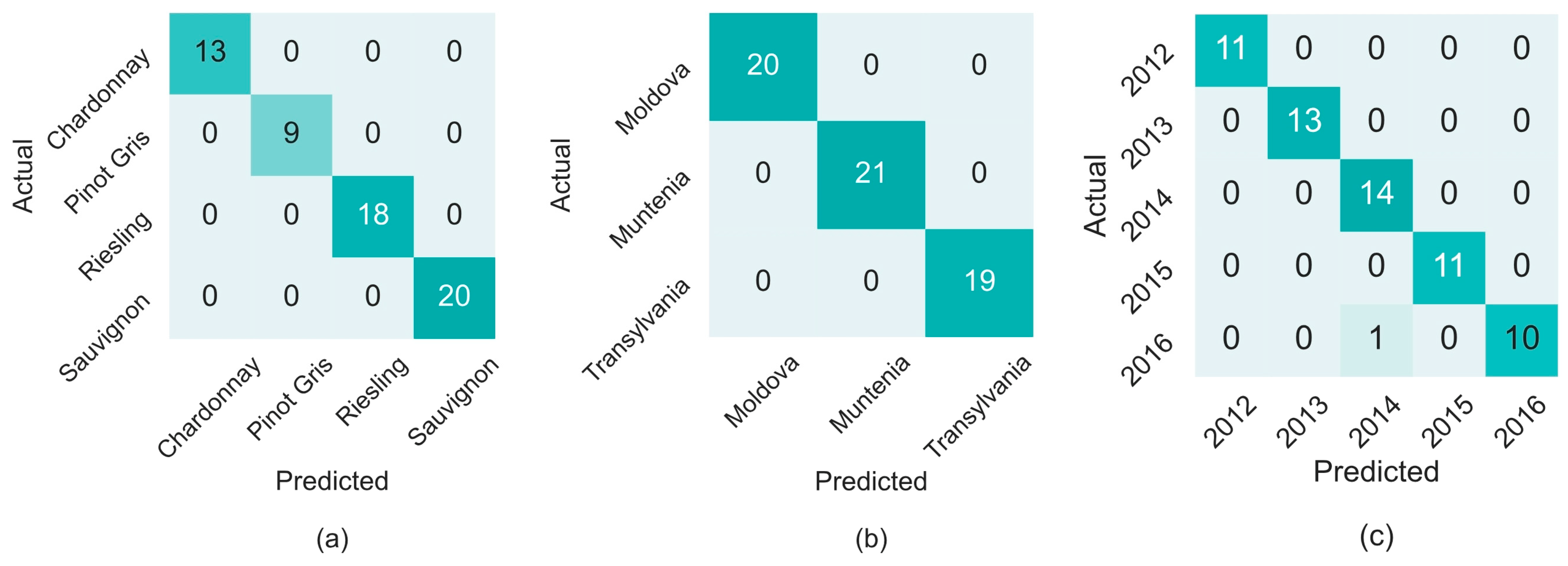
3.2. Varietal Differentiation

The first category of prediction models was developed for classifying the wine samples with respect to the following cultivars: Chardonnay, Pinot Gris, Riesling, and Sauvignon. In this regard, as previously mentioned, the first step in the working flow (Figure 2) consisted of the application of distinct preprocessing techniques on the raw spectra (i.e., autoscale, Pareto, variance scaling, row-wise min–max scaling, and column-wise min–max scaling). The impact of each method was evaluated through the performance of PLS-DA models that had the transformed spectra of the training samples as input data. Using the entire mentioned spectral region, modest accuracies, based on 10-fold cross-validation, were obtained, as can be seen in Table 1. However, after the application of the data dimensionality reduction step based on PLS for identifying the meaningful variables for the proposed classification, a drastic decrease in the input space dimensionality was achieved. According to the information presented in Table 2, the preprocessing methods that led to the selection of the lowest number of spectral points corresponded to autoscale and variance scaling. These outcomes are in good agreement with the results obtained in the frame of previously published papers [25,31], where the suitability of applying variance scaling or autoscaling for transforming the raw 1H-NMR spectra of wine [31] or other food matrices such as honey [25] was highlighted. These techniques led to the extraction of approximately 1% of the points from the entire utilized spectral range (i.e., between 0 and 10 ppm), whereas the other three methods led to the extraction of between 4% and 55% of the variables. New PLS-DA models were subsequently constructed based on the information stored only in the meaningful spectral points. Through this approach, mean accuracy scores between 35% and 100% were obtained in the cross-validation procedure (Table 2). Autoscale and variance scaling were the preprocessing methods that allowed a perfect simultaneous discrimination of the four cultivars, which might be linked to the fact that the feature selection method applied to the data preprocessed through these techniques led to the highest decrease in the dimensionality of the input space (i.e., from 18,181 to 210 spectral points for autoscale and to 176 variables in the case of variance scaling).
Based on the results obtained from the conducted preprocessing investigations regarding varietal discrimination, the input data for the development of the machine learning models corresponded to the 176 variables transformed through variance scaling (Figure S1), which were selected by the feature selection algorithm. In this regard, a tentative attribution of the obtained markers based on the reported literature [32] indicated that the differentiation of the wine samples concerning the cultivar is due to the following compounds: tyrosine (6.89 and 7.17 ppm), proline (1.99, 2.06, 2.33, 3.32, and 4.11 ppm), caffeic acid (6.43 and 7.69 ppm), alanine (1.48 and 3.76 ppm), pyruvic acid (2.35 ppm), and gallic acid (7.13 ppm). These findings are consistent with the most significant differentiators found in the frame of previous studies [26,31,32,33] between several wine varieties.
Using this optimal input data space, the application of Logistic Regression allowed a perfect prediction of all the investigated training wine samples in regard to the cultivar, conducting to a mean accuracy score of 100% in the cross-validation evaluation procedure (Figure 3a and Figure S2a). The optimized classification model was characterized by a liblinear solver, an L2 penalty, and a C parameter of 3792.6. In addition, the maximum number of iterations allowed for convergence was set to 100. This selection of hyperparameters illustrated the best performance based on the accuracy metric.
The learning-based classifier illustrating this configuration was further retrained based on the entire training set and subjected to a testing phase, proving its high capacity in recognizing the cultivar of the wine samples through the achievement of a 100% accuracy rate. In this case, all five test samples, namely three Sauvignon Blanc and two Riesling samples, were correctly classified by the developed Logistic Regression model.
In comparison with Logistic Regression, the kNN algorithm was shown to be less efficient in classifying wines according to the varietal origin. The optimized model led to the accurate prediction of 81% of the wine samples, leading to a sensitivity score of 100% for the Riesling class, and of 90%, 84%, and 22% for the Sauvignon, Chardonnay, and Pinot Gris groups, respectively. The low probability of detection of the Pinot Gris class was mainly due to the misclassification of five wine samples belonging to this cultivar to the Riesling group. The kNN algorithm utilized the Euclidean metric for computing the distance, the points were weighted equally, and the number of neighbors was set to 3. A similar accuracy was also achieved in the test phase, when the kNN classifier correctly identified the variety of 80% of the samples, with one Sauvignon Blanc wine being wrongly attributed to the Chardonnay class.

3.3. Geographical Classification

For the geographical differentiation of the wine samples, the same data processing workflow, as illustrated in Figure 2, was adopted as in the case of varietal classification. Firstly, the most efficient input data aimed to be identified by means of testing distinct preprocessing techniques and comparing them through the application of a supervised statistical method, namely PLS-DA. In this regard, the raw spectra of the training instances were transformed using the following methods: autoscale, Pareto, variance scaling, min–max scaling (applied to rows), and min–max scaling (applied to columns). In cases when the input data consisted of the entire spectral range (Table 1), accuracy scores between 36% and 60% were obtained. Even though these classification models were observed to be more efficient for identifying the geographical source of the Transylvanian samples, the overall classification results were not reliable. To improve the discrimination ability of the discrimination models, the PLS-based feature selection technique was applied. Through this method, the input data space was limited to the most relevant geographical markers, leading to a significant decrease in the variable number, especially when the 1H-NMR experimental spectra were preprocessed with Pareto, autoscale, column-wise min–max scaling, and variance scaling (Table 2). The highest performance (100% accuracy) was obtained for the data preprocessed with variance scaling, followed by autoscaling, a case in which 98% of the wine samples were properly classified with respect to the geographical origin. Once again, these two data pretreatment techniques, found to be the most effective for transforming the raw 1H-NMR wine spectra, are consistent with the preprocessing results highlighted in previous studies [25,31]. This 98% accuracy obtained by the autoscaled input data occurred due to the fact that one sample from Moldova was misclassified and attributed to the Muntenia class (Table 2).
Having this insight about the data input space, the selected variables for the development of the machine learning models corresponded to the 800 attributes that were identified as relevant markers when variance scaling was applied to the 1H-NMR spectra (Figure S3). To assess the significance of the identified features, a preliminary attribution of the 1H-NMR spectral variables to the molecules responsible for their corresponding signal was performed, guided by peak attributions previously reported in the literature [32]. Accordingly, the markers identified for geographical discrimination appeared to be associated with the following compounds: tyrosine (6.89 and 7.17 ppm), phenethyl alcohol (2.76, 3.74, 7.28, and 7.34 ppm), trigonelline (8.07, 8.82, and 9.11 ppm), fumaric acid (6.71 ppm), shikimic acid (6.81 ppm), tartaric acid (4.41 ppm), succinic acid (2.62 ppm), caffeic acid (6.43 and 7.69 ppm), alanine (1.48 and 3.76 ppm), pyruvic acid (2.35 ppm), and gallic acid (7.13 ppm). The alignment of these differentiator markers with the ones emphasized in previously reported studies [26,31,32] indicates that the employed methodology effectively captured the key geographical characteristics from the 1H-NMR spectra.
Based on these input data, the Logistic Regression algorithm conducted the obtainment of a 100% cross-validation accuracy score in classifying the Romanian wine sample set in regard to the region of production (Figure 3b and Figure S1b). In this case, the optimized model for this task illustrated the use of a liblinear solver, an L1 penalty, a C parameter of 10,000, and had the maximum number of iterations set to 2500. The model also illustrated a high performance during the testing phase, when four out of five samples were correctly predicted in terms of the region of production. Correspondingly, only one wine sample produced in Moldova was misclassified and attributed to the Muntenia region.
Despite its simplicity, the kNN algorithm correctly predicted 83% of the wine samples according to geographical origin; namely, 94% of the samples from the Transylvania region were properly classified, 80% of those originating from Muntenia were correctly predicted, while a lower precision measure of 75% was obtained for the Moldova class. As resulted from the grid-search approach conducted for tuning the hyperparameters, the kNN model was characterized by a number of 3 neighbors, the Euclidean function, and a distance weight function (i.e., the influence of neighbors diminished as the distance from the query point increased).

3.4. Harvesting Year Discrimination

The last investigated wine sample differentiation was made according to the vintage. The purpose was to find the best discrimination model able to recognize the wine samples produced over five consecutive years: 2012–2016. For identifying the most suitable input data for developing the harvesting year differentiation models, the same approach was conducted as for the previous classification criteria (Figure 2). Once again, the utilization of the entire 1H-NMR spectral range (i.e., 18,181 data points) obtained poor classification results when PLS-DA models were constructed, no matter the applied preprocessing technique (Table 1). However, after the data dimensionality reduction step, high accuracy scores in recognizing the wine samples’ harvesting year were achieved when the experimental data were previously preprocessed by autoscaling and variance scaling. It was observed that for these two types of data preprocessing methods, the dimensionality reduction process proved to be very efficient; namely, it led to the identification of a small number of relevant discrimination variables as opposed to the original input data space. Thus, a decrease from 18,181 to 252 variables was obtained for the data set preprocessed with autoscale, and this reduction was comparable with the one realized when the variance (std) scaling method was used, where a total of 277 variables proved to have the highest discrimination power for this classification (Table 2).
For consistency reasons, the selected input data for constructing machine learning models were represented by the 277 markers identified when the experimental data were preprocessed through variance scaling (Figure S4). Based on the peak assignments reported in the literature [32], the 1H-NMR markers that allowed the vintage discrimination of the wine samples were as follows: tyrosine (6.89 and 7.17 ppm), phenethyl alcohol (2.76, 3.74, 7.28, and 7.34 ppm), succinic acid (2.62 ppm), proline (1.99, 2.06, 2.33, 3.32, and 4.11 ppm), caffeic acid (6.43 and 7.69 ppm), alanine (1.48 and 3.76 ppm), and pyruvic acid (2.35 ppm). Tyrosine, phenethyl alcohol, succinic acid, proline, and caffeic acid have also been reported as relevant markers for vintage discrimination in the previous work [31].
Once again, the application of Logistic Regression for wine classification allowed the obtainment of highly reliable results. The model, defined through a liblinear solver, an L1 penalty, a C parameter of 10,000, and having the maximum number of iterations set to 5000, correctly predicted 98% of the samples (Figure 3c and Figure S2c). For this differentiation, only one sample was misclassified; namely, a wine produced in 2016 was attributed to the 2014 vintage. This recognition performance is of high relevance since the investigated vintage classification refers to the simultaneous differentiation of 5 consecutive years and comprises wines from various production regions, characterized by different geoclimatic characteristics and corresponding to different cultivars. Nonetheless, the performance of the model was finally assessed in regard to the test instances, which allowed the correct attribution of three samples out of five. In this case, one sample produced in 2012 and another one from 2014 were wrongly labeled as samples from the 2013 production year.
In the case when the kNN algorithm was applied, a lower performance in classifying wines according to the vintage was recorded in cross-validation. In this case, a 68% accuracy measure was obtained and sensitivity scores of 72%, 76%, 64%, 100%, and 27% were obtained for 2012, 2013, 2014, 2015, and 2016 vintages, respectively. The kNN model was characterized by a number of 13 neighbors, a uniform weight function, and the Euclidean distance function, as a result of the hyperparameter tuning process. Despite illustrating a much lower prediction ability in cross-validation, the kNN model led to the obtainment of the same prediction performance concerning the test set as the Logistic Regression classifier; namely, three out of five samples were correctly classified in terms of harvesting year.
Based on a search conducted on the Web of Knowledge in January 2025, in the literature, no research studies have been previously reported for investigating the potential of utilizing 1H-NMR in association with Logistic Regression or kNN algorithms for predicting the origin of wine. In this regard, the originality of the present study emerges particularly from the meticulous optimization of the data processing workflow for the development of reliable wine authentication models based on these modeling techniques. The application of 1H-NMR spectroscopy for wine recognition through the employment of chemometric or other learning-based methods has also been proposed in the studies [23,26,31,34]. For example, Fan et al. [34] discussed the potential of applying 1H-NMR in association with multivariate statistical analysis for discriminating in regard to the variety a data set comprising 170 Chinese wine samples originating from different regions in China and harvested in different years. The classification performances reported by the authors were 82% and 94% in internal validation and 83% and 94% in testing, for red and white wine, respectively. The higher accuracy scores obtained for the cultivar discrimination in the frame of our study (i.e., 100% in internal validation and 100% in testing on an independent sample set) might be the outcome of the application of a supervised method for selecting the relevant variables for a specific classification criterion or of the in-depth optimization process conducted for selecting the Logistic Regression’s hyperparameters. Higher classification accuracies were also achieved in comparison with our previously published paper [31], where we aimed to differentiate a data set of 55 wine samples concerning the geographical origin, cultivar, and vintage. As was proven in the present study, where a direct comparison between two distinct ML algorithms was performed, the explanation for the achieved performance improvement can be attributed to the utilization of a more suitable learning-based algorithm for the present task. However, performing a comparison between the approaches proposed in the frame of the present study and similar ones reported in the literature is challenging, mainly owing to the fact that the data sets employed for constructing the classification models are different. The variations can arise from numerous aspects, including the number of wine samples, the considered geographical regions, wine varieties, and vintages, or even the employed data preprocessing methods that directly influence the input data for the development of the prediction models.

4. Conclusions

The present work highlighted the potential given by machine learning methods for differentiating wine samples with respect to the cultivar, geographical origin, and harvesting year, based on the experimental data obtained through 1H-NMR spectroscopy. In this regard, k-Nearest Neighbors and Logistic Regression were applied for the development of the prediction models. With the aim of constructing reliable wine control instruments, an emphasis was placed on the utilization of an appropriate preprocessing method for transforming the raw 1H-NMR spectra, along with the selection of the most significant variables, identified individually for each differentiation type. For all the investigated classification criteria, the algorithm that allowed the development of the prediction models having the highest performance (i.e., greater than 98% mean accuracy in the 10-fold cross-validation procedure and between 60% and 100% in testing) proved to be Logistic Regression. These results were achieved when the raw experimental data were preprocessed through variance scaling and the dimensionality of the input space was drastically reduced. Moreover, our study proposes an optimum workflow for the successful association between 1H-NMR spectroscopy and machine learning algorithms. In this flow, we pointed out the importance of the data preprocessing phase, with an emphasis on feature selection. Based on the proposed approach, reliable wine recognition models have been constructed for all wine differentiation criteria: vintage, cultivar, and geographical origin.

Supplementary Materials

The following supporting information can be downloaded at: https://www.mdpi.com/article/10.3390/beverages11020045/s1, Table S1: Distribution of training and test samples in regard to the cultivars, geographical origins and vintages; Figure S1: Most efficient discriminant markers found for the cultivar classification of the wine samples based on the 1H-NMR spectra preprocessed through variance (std) scaling; Figure S2. Cross-validation probability estimates returned by the most optimal Logistic Regression model developed for classifying the wine samples with respect to the (a) cultivar, (b) geographical origin, and (c) vintage; Figure S3. 1H-NMR variables identified as the most efficient geographical discriminators of the wine samples when variance (std) scaling was used for preprocessing the raw spectra; Figure S4. 1H-NMR spectral points identified as most relevant for the discrimination of the wine samples according to the vintage.

Author Contributions

Conceptualization, D.A.M.; methodology, A.P.; software, A.R.H.; validation, A.R.H. and D.A.M.; formal analysis, A.P.; investigation, A.P.; resources, D.A.M.; data curation, A.R.H. and A.P.; writing—original draft preparation, A.R.H. and D.A.M.; writing—review and editing, A.R.H., A.P. and D.A.M.; visualization, A.R.H.; supervision, D.A.M.; project administration, D.A.M.; funding acquisition, D.A.M. All authors have read and agreed to the published version of the manuscript.

Funding

This paper was co-financed by the European Regional Development Fund (ERDF) through the Smart Growth, Digitization and Financial Instruments Program (PoCIDIF), call PCIDIF/144/PCIDIF_P1/OP1/RSO1.1/PCIDIF_A3, Project SMIS number 309287, acronym METROFOOD-RO Evolve.

Data Availability Statement

The data presented in this study are available on request from the corresponding author.

Conflicts of Interest

The authors declare no conflicts of interest.

References

  1. Moore, J.C.; Spink, J.; Lipp, M. Development and application of a database of food ingredient fraud and economically motivated adulteration from 1980 to 2010. J. Food Sci. 2012, 77, R118–R126. [Google Scholar] [CrossRef]
  2. Solovyev, P.A.; Fauhl-Hassek, C.; Riedl, J.; Esslinger, S.; Bontempo, L.; Camin, F. NMR spectroscopy in wine authentication: An official control perspective. Compr. Rev. Food Sci. Food Saf. 2021, 20, 2040–2062. [Google Scholar] [CrossRef]
  3. Jackson, R.S. Chapter 6—Chemical constituents of grapes and wine. In Wine Science, 5th ed.; Jackson, R.S., Ed.; Academic Press: Cambridge, MA, USA, 2020; pp. 375–459. [Google Scholar] [CrossRef]
  4. Sun, X.; Zhang, F.; Gutiérrez-Gamboa, G.; Ge, Q.; Xu, P.; Zhang, Q.; Fang, Y.; Ma, T. Real Wine or Not? Protecting Wine with Traceability and Authenticity for Consumers: Chemical and Technical Basis, Technique Applications, Challenge, and Perspectives. Crit. Rev. Food Sci. Nutr. 2021, 62, 6783–6808. [Google Scholar] [CrossRef] [PubMed]
  5. Koljančić, N.; Furdíková, K.; de Araújo Gomes, A.; Špánik, I. Wine authentication: Current progress and state of the art. Trends Food Sci. Technol. 2024, 150, 104598. [Google Scholar] [CrossRef]
  6. Camin, F.; Boner, M.; Bontempo, L.; Fauhl-Hassek, C.; Kelly, S.D.; Riedl, J.; Rossmann, A. Stable isotope techniques for verifying the declared geographical origin of food in legal cases. Trends Food Sci. Technol. 2017, 61, 176–187. [Google Scholar] [CrossRef]
  7. Basalekou, M.; Pappas, C.; Tarantilis, P.; Kotseridis, Y.; Kallithraka, S. Wine authentication with Fourier Transform Infrared Spectroscopy: A feasibility study on variety, type of barrel wood and ageing time classification. Int. J. Food Sci. 2017, 52, 1307–1313. [Google Scholar] [CrossRef]
  8. Lu, B.; Tian, F.; Chen, C.; Wu, W.; Tian, X.; Chen, C.; Lv, X. Identification of Chinese red wine origins based on Raman spectroscopy and deep learning. Spectrochim. Acta Part A Mol. Biomol. Spectrosc. 2023, 291, 122355. [Google Scholar] [CrossRef]
  9. Bevin, C.J.; Dambergs, R.G.; Fergusson, A.J.; Cozzolino, D. Varietal discrimination of Australian wines by means of mid-infrared spectroscopy and multivariate analysis. Anal. Chim. Acta 2008, 621, 19–23. [Google Scholar] [CrossRef]
  10. Magdas, D.A.; Cinta Pinzaru, S.; Guyon, F.; Feher, I.; Cozar, B.I. Application of SERS technique in white wines discrimination. Food Control 2018, 92, 30–36. [Google Scholar] [CrossRef]
  11. Godelmann, R.; Fang, F.; Humpfer, E.; Schütz, B.; Bansbach, M.; Schäfer, H.; Spraul, M. Targeted and nontargeted wine analysis by 1H NMR spectroscopy combined with multivariate statistical analysis. Differentiation of important parameters: Grape variety, geographical origin, year of vintage. J. Agric. Food Chem. 2013, 61, 5610–5619. [Google Scholar] [CrossRef]
  12. Anastasiadi, M.; Zira, A.; Magiatis, P.; Haroutounian, S.A.; Skaltsounis, A.L.; Mikros, E. 1H NMR-based metabonomics for the classification of Greek wines according to variety, region, and vintage. Comparison with HPLC data. J. Agric. Food Chem. 2009, 57, 11067–11074. [Google Scholar] [CrossRef] [PubMed]
  13. Ehlers, M.; Horn, B.; Raeke, J.; Fauhl-Hassek, C.; Hermann, A.; Brockmeyer, J.; Riedl, J. Towards harmonization of non-targeted 1H NMR spectroscopy-based wine authentication: Instrument comparison. Food Control 2022, 132, 108508. [Google Scholar] [CrossRef]
  14. Suciu, R.C.; Zarbo, L.; Guyon, F.; Magdas, D.A. Application of fluorescence spectroscopy using classical right angle technique in white wines classification. Sci. Rep. 2019, 9, 18250. [Google Scholar] [CrossRef] [PubMed]
  15. Azcarate, S.M.; de Araújo Gomes, A.; Alcaraz, M.R.; de Araújo, M.C.U.; Camiña, J.M.; Goicoechea, H.C. Modeling excitation–emission fluorescence matrices with pattern recognition algorithms for classification of Argentine white wines according grape variety. Food Chem. 2015, 184, 214–219. [Google Scholar] [CrossRef]
  16. Ranaweera, R.K.R.; Capone, D.L.; Bastian, S.E.P.; Cozzolino, D.; Jeffery, D.W. A Review of Wine Authentication Using Spectroscopic Approaches in Combination with Chemometrics. Molecules 2021, 26, 4334. [Google Scholar] [CrossRef]
  17. Friebolin, H. Basic One-and Two-Dimensional NMR Spectroscopy, 4th ed.; Wiley-VCH: Weinheim, Germany, 2005. [Google Scholar]
  18. Lolli, V.; Caligiani, A. How NMR contributes to food authentication: Current trends and perspectives. Curr. Opin. Food Sci. 2024, 58, 101200. [Google Scholar] [CrossRef]
  19. Balthazar, C.F.; Guimarães, J.T.; Rocha, R.S.; Pimentel, T.C.; Neto, R.P.C.; Tavares, M.I.B.; Graça, J.S.; Alves Filho, E.G.; Freitas, M.Q.; Esmerino, E.A.; et al. Nuclear Magnetic Resonance as an Analytical Tool for Monitoring the Quality and Authenticity of Dairy Foods. Trends Food Sci. Technol. 2021, 108, 84–91. [Google Scholar] [CrossRef]
  20. Smolinska, A.; Blanchet, L.; Buydens, L.M.C.; Wijmenga, S.S. NMR and pattern recognition methods in metabolomics: From data acquisition to biomarker discovery: A review. Anal. Chim. Acta 2012, 750, 82–97. [Google Scholar] [CrossRef]
  21. Mitchell, T.M. Machine Learning; McGraw-Hill: New York, NY, USA, 1997. [Google Scholar]
  22. Jordan, M.I.; Mitchell, T.M. Machine learning: Trends, perspectives, and prospects. Science 2015, 349, 255–260. [Google Scholar] [CrossRef]
  23. Mascellani, A.; Hoca, G.; Babisz, M.; Krska, P.; Kloucek, P.; Havlik, J. 1H NMR chemometric models for classification of Czech wine type and variety. Food Chem. 2021, 339, 127852. [Google Scholar] [CrossRef]
  24. Esslinger, S.; Fauhl-Hassek, C.; Wittkowski, R. Authentication of Wine by 1H-NMR Spectroscopy: Opportunities and Challenges. In Advances in Wine Research; Ebeler, S.B., Sacks, G., Vidal, S., Winterhalter, P., Eds.; American Chemical Society: Washington, DC, USA, 2015; pp. 85–108. [Google Scholar]
  25. Hategan, A.R.; Guyon, F.; Magdas, D.A. The improvement of honey recognition models built on 1H NMR fingerprint through a new proposed approach for feature selection. J. Food Compos. Anal. 2022, 114, 104786. [Google Scholar] [CrossRef]
  26. Magdas, D.A.; Pirnau, A.; Feher, I.; Guyon, F.; Cozar, B.I. Alternative approach of applying 1H NMR in conjunction with chemometrics for wine classification. LWT 2019, 109, 422–428. [Google Scholar] [CrossRef]
  27. Roger, J.M.; Boulet, J.C.; Zeaiter, M.; Rutledge, D.N. Pre-processing methods. In Comprehensive Chemometrics; Brown, S., Tauler, R., Walczak, B., Eds.; Elsevier: Oxford, UK, 2020; pp. 1–75. [Google Scholar]
  28. Eigenvector Research Wiki, Selectvars. Available online: https://wiki.eigenvector.com/index.php?title=Selectvars (accessed on 22 November 2024).
  29. Pedregosa, F.; Varoquaux, G.; Gramfort, A.; Michel, V.; Thirion, B.; Grisel, O.; Blondel, M.; Prettenhofer, P.; Weiss, R.; Dubourg, V.; et al. Scikit-learn: Machine learning in Python. J. Mach. Learn. Res. 2011, 12, 2825–2830. [Google Scholar]
  30. Bisong, E. Logistic Regression. In Building Machine Learning and Deep Learning Models on Google Cloud Platform; Apress: Berkeley, CA, USA, 2019. [Google Scholar] [CrossRef]
  31. Hategan, A.R.; David, M.; Pirnau, A.; Cozar, B.; Cinta-Pinzaru, S.; Guyon, F.; Magdas, D.A. Fusing 1H NMR and Raman experimental data for the improvement of wine recognition models. Food Chem. 2024, 458, 140245. [Google Scholar] [CrossRef]
  32. Gougeon, L.; Da Costa, G.; Le Mao, I.; Ma, W.; Teissedre, P.L.; Guyon, F.; Richard, T. Wine analysis and authenticity using 1H-NMR metabolomics data: Application to Chinese wines. Food Anal. Methods 2018, 11, 3425–3434. [Google Scholar] [CrossRef]
  33. Bambina, P.; Spinella, A.; Lo Papa, G.; Chillura Martino, D.F.; Lo Meo, P.; Cinquanta, L.; Conte, P. 1H-NMR Spectroscopy Coupled with Chemometrics to Classify Wines According to Different Grape Varieties and Different Terroirs. Agriculture 2024, 14, 749. [Google Scholar] [CrossRef]
  34. Fan, S.; Zhong, Q.; Fauhl-Hassek, C.; Pfister, M.K.H.; Horn, B.; Huang, Z. Classification of Chinese wine varieties using 1H NMR spectroscopy combined with multivariate statistical analysis. Food Control 2018, 88, 113–122. [Google Scholar] [CrossRef]
Figure 1. Details of stacked 1H-NMR spectra of wine samples belonging to distinct cultivars.
Beverages 11 00045 g001
Figure 2. Data processing workflow for wine recognition model development.
Beverages 11 00045 g002
Figure 3. Confusion matrices corresponding to the cross-validation predictions of the optimized Logistic Regression models in regard to the (a) cultivar, (b) geographical, and (c) vintage classifications of the wine samples.
Beverages 11 00045 g003
Table 1. Performance of PLS-DA models aiming the discrimination of wine based on the 1H-NMR spectral range of 0–10 ppm as a function of the classification criterion (i.e., cultivar, geographical origin, and vintage) and the type of preprocessing.
Preprocessing MethodNumber of VariablesTrue PositivesAccuracy
(CV)
Cultivar discrimination
Chardonnay
(13)
Pinot Gris
(9)
Riesling
(18)
Sauvignon
(20)
autoscale18,181638120.48
Pareto18,18155570.36
variance scaling18,181611290.46
min–max scaling (row-wise)18,18161670.33
min–max scaling (column-wise)18,181511350.40
Geographical origin discrimination
Moldova
(20)
Muntenia
(21)
Transylvania
(19)
autoscale18,181714150.60
Pareto18,18187130.46
variance scaling18,181911150.58
min–max scaling (row-wise)18,18184100.36
min–max scaling (column-wise)18,181616130.58
Vintage discrimination
2012
(11)
2013
(13)
2014
(14)
2015
(11)
2016
(11)
autoscale18,181456550.41
Pareto18,181425310.25
variance scaling18,181436320.30
min–max scaling (row-wise)18,181655720.41
min–max scaling (column-wise)18,181637120.31
Table 2. The 10-fold cross-validation performance of the PLS-DA models developed based on the selected variables as a function of the classification criterion and the method used for preprocessing the raw 1H-NMR spectra.
Preprocessing MethodNumber of VariablesTrue PositivesAccuracy
(CV)
Cultivar discrimination
Chardonnay
(13)
Pinot Gris
(9)
Riesling
(18)
Sauvignon
(20)
autoscale21013918201.00
Pareto9156413100.55
variance scaling17613918201.00
min–max scaling (row-wise)10,00063570.35
min–max scaling (column-wise)73411616170.83
Geographical origin discrimination
Moldova
(20)
Muntenia
(21)
Transylvania
(19)
autoscale5121921190.98
Pareto2771317140.73
variance scaling8002021191.00
min–max scaling (row-wise)302512780.45
min–max scaling (column-wise)5091920140.88
Vintage discrimination
2012
(11)
2013
(13)
2014
(14)
2015
(11)
2016
(11)
autoscale25211131311110.98
Pareto503469850.53
variance scaling27711121411110.98
min–max scaling (row-wise)152516750.40
min–max scaling (column-wise)18,181637120.31
Disclaimer/Publisher’s Note: The statements, opinions and data contained in all publications are solely those of the individual author(s) and contributor(s) and not of MDPI and/or the editor(s). MDPI and/or the editor(s) disclaim responsibility for any injury to people or property resulting from any ideas, methods, instructions or products referred to in the content.

