Compressive Mechanical Properties of Porcine Brain: Experimentation and Modeling of the Tissue Hydration Effects

 , , ,
, , , 

Abstract
: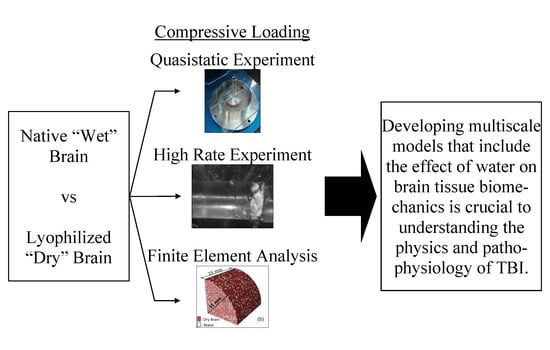
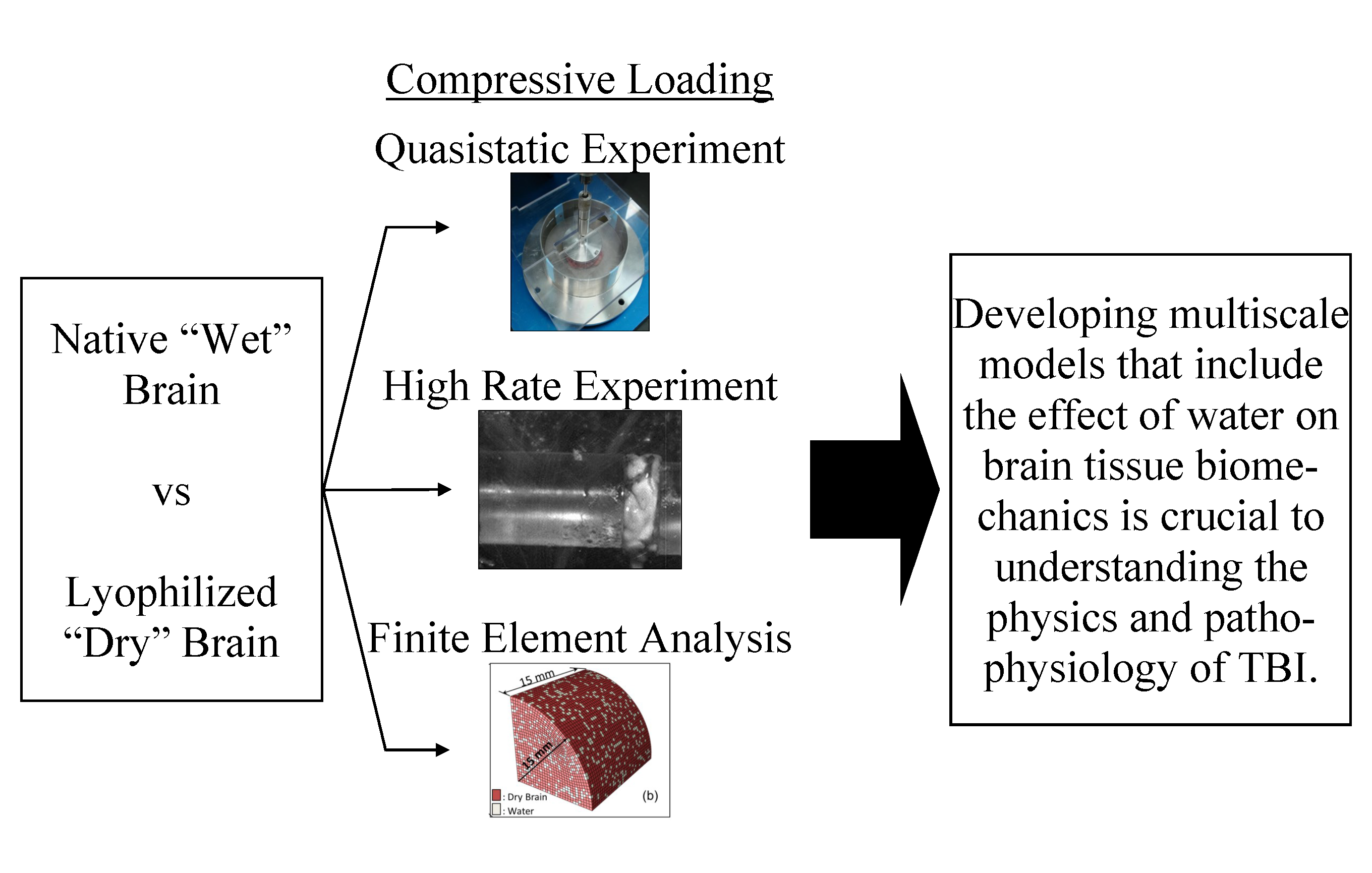
1. Introduction
2. Materials and Methods
2.1. Sample Preparation
2.2. Testing Apparatuses
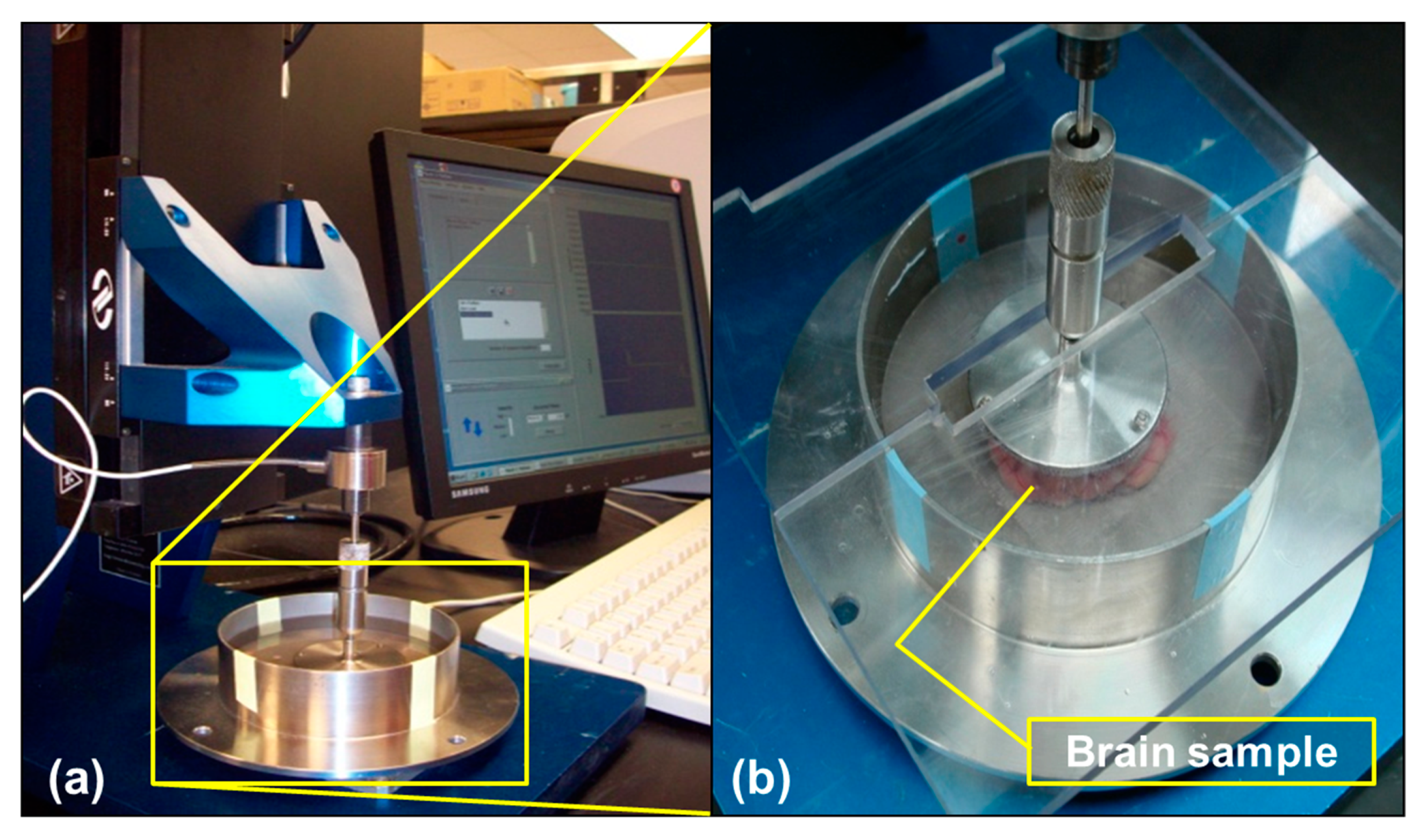
2.2.1. Mach-1™ for Quasi-static Testing of the Wet Brain
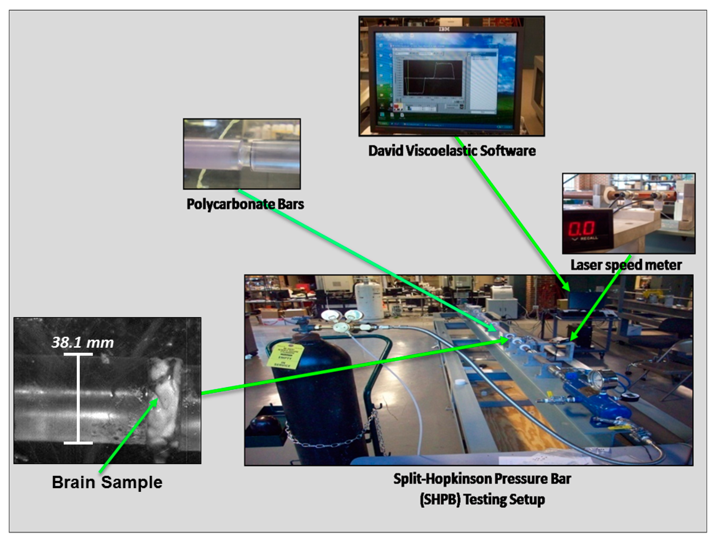
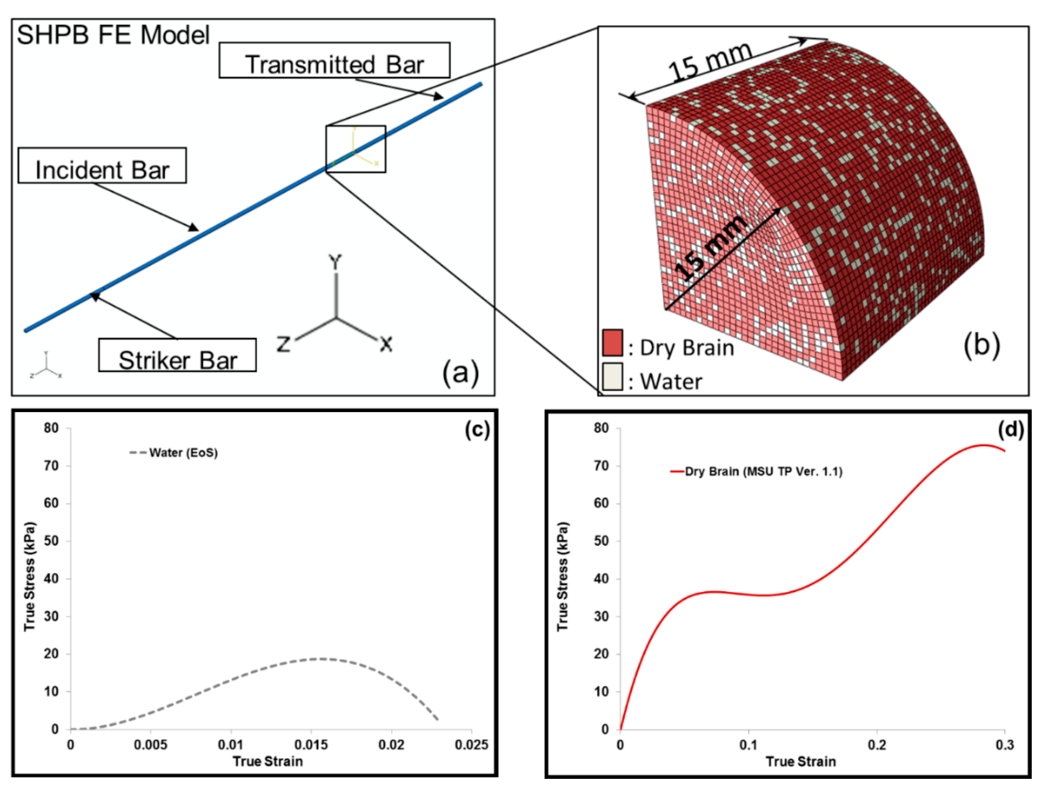
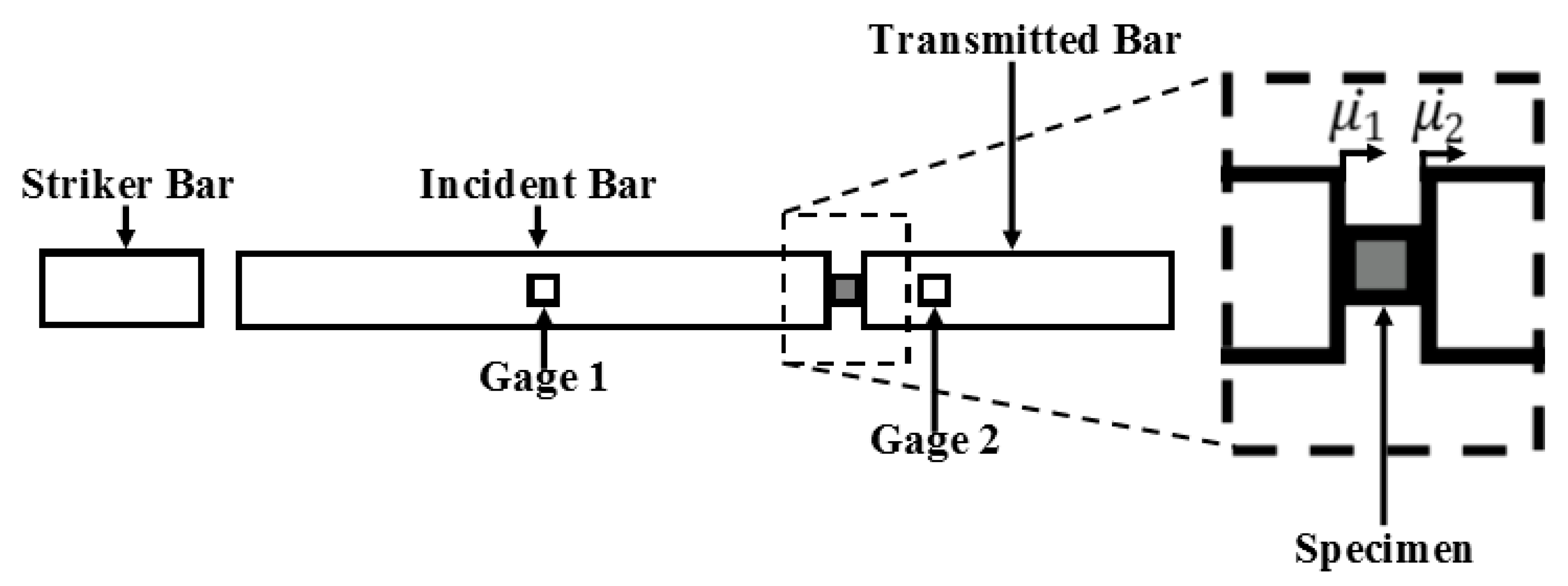
2.2.2. Split-Hopkinson Pressure Bar (SHPB) for High Strain Rate Testing of Wet and Dry Brain Specimens
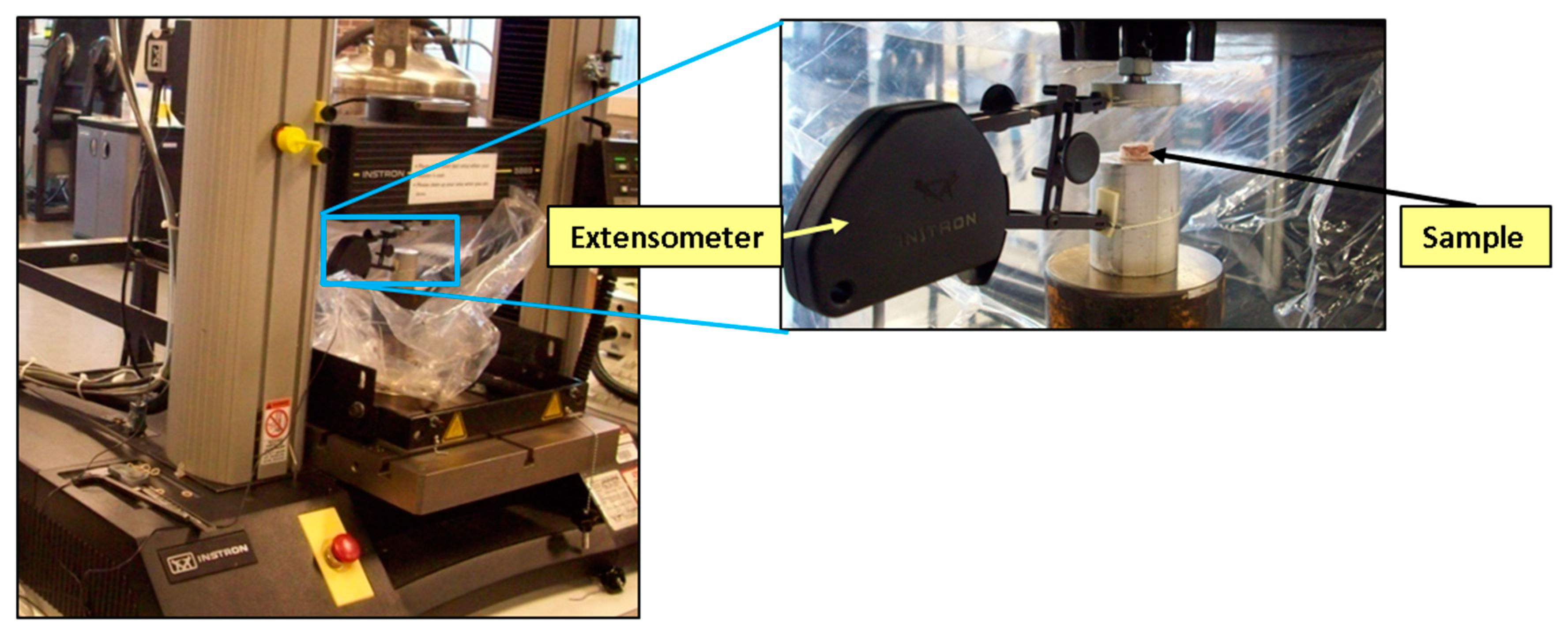
2.2.3. Instron™5568 for Quasi-Static Testing of the Dry Brain
2.3. Stress–Strain Experimental Data
2.4. Statistical Analysis of the Experimental Data
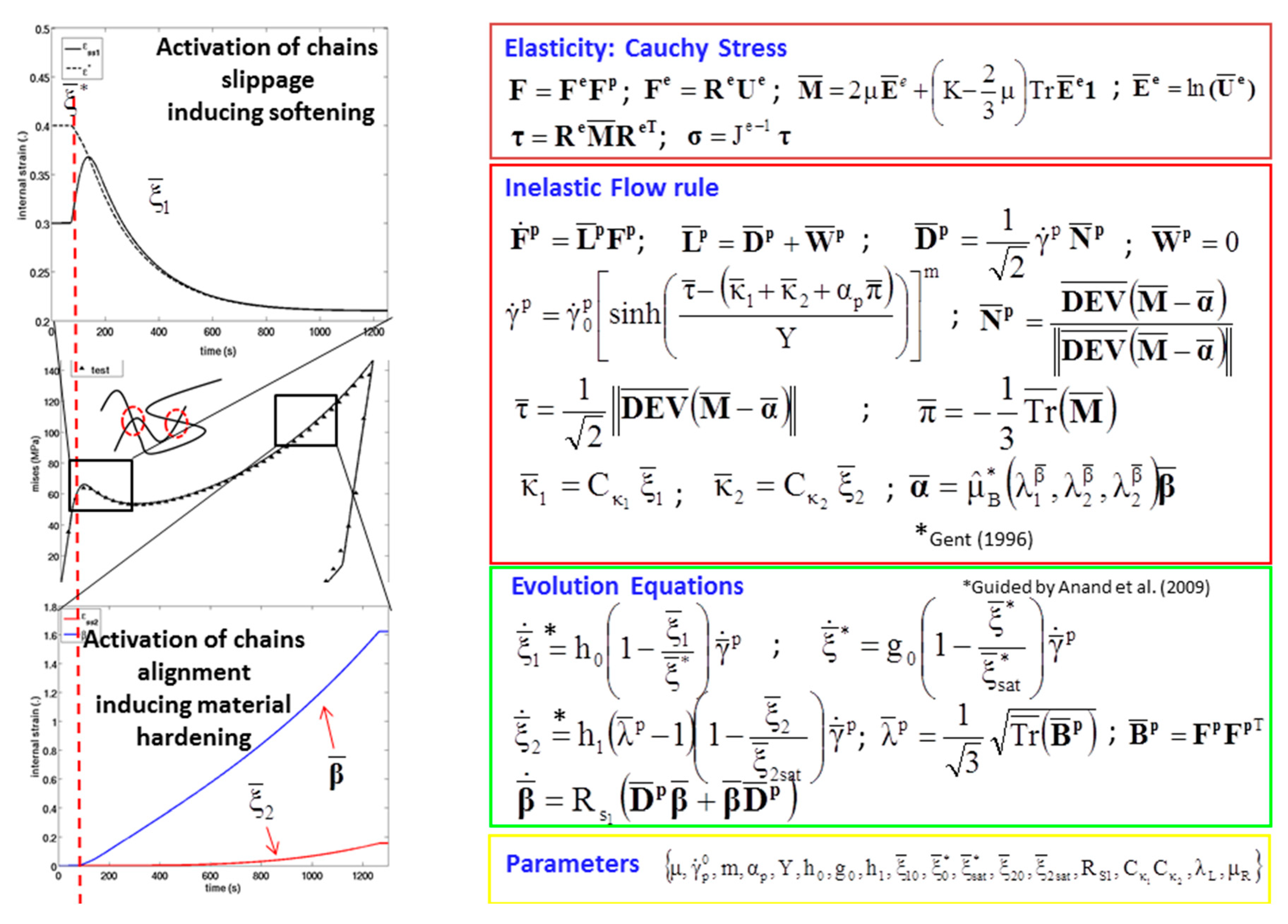
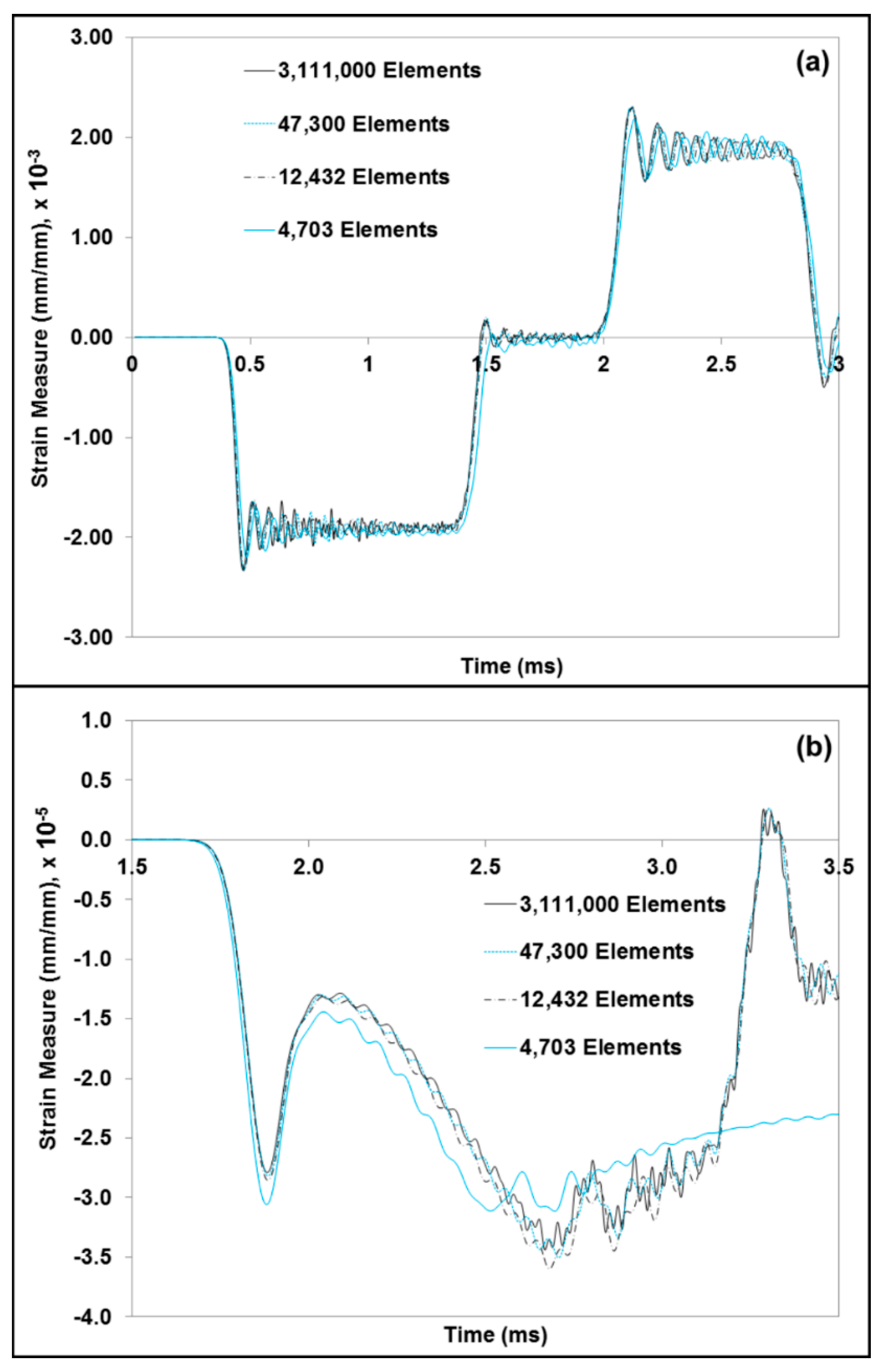
2.5. Finite Element Simulation-Based Micromechanics of the Dry Brain and Water
3. Results and Discussion
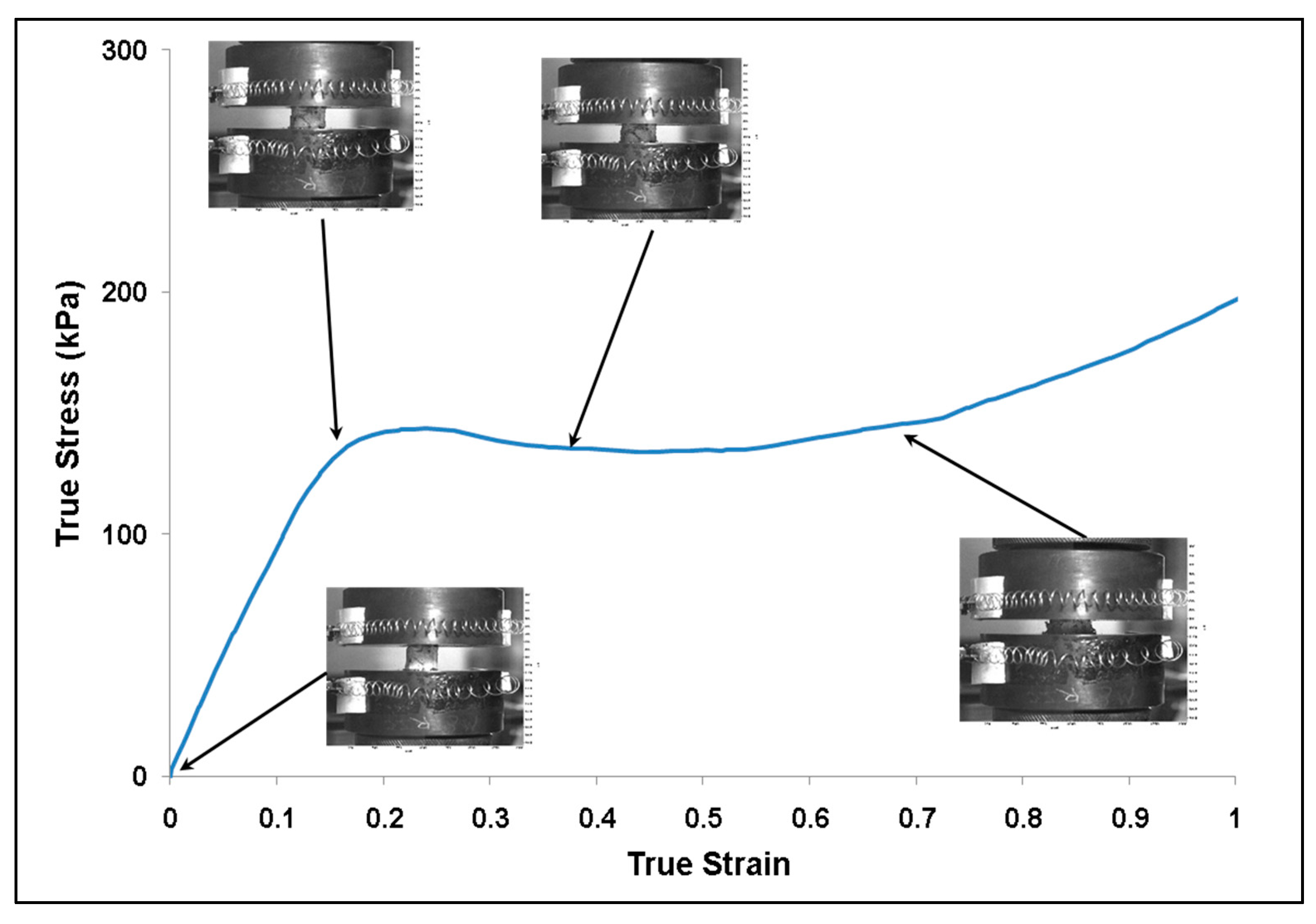
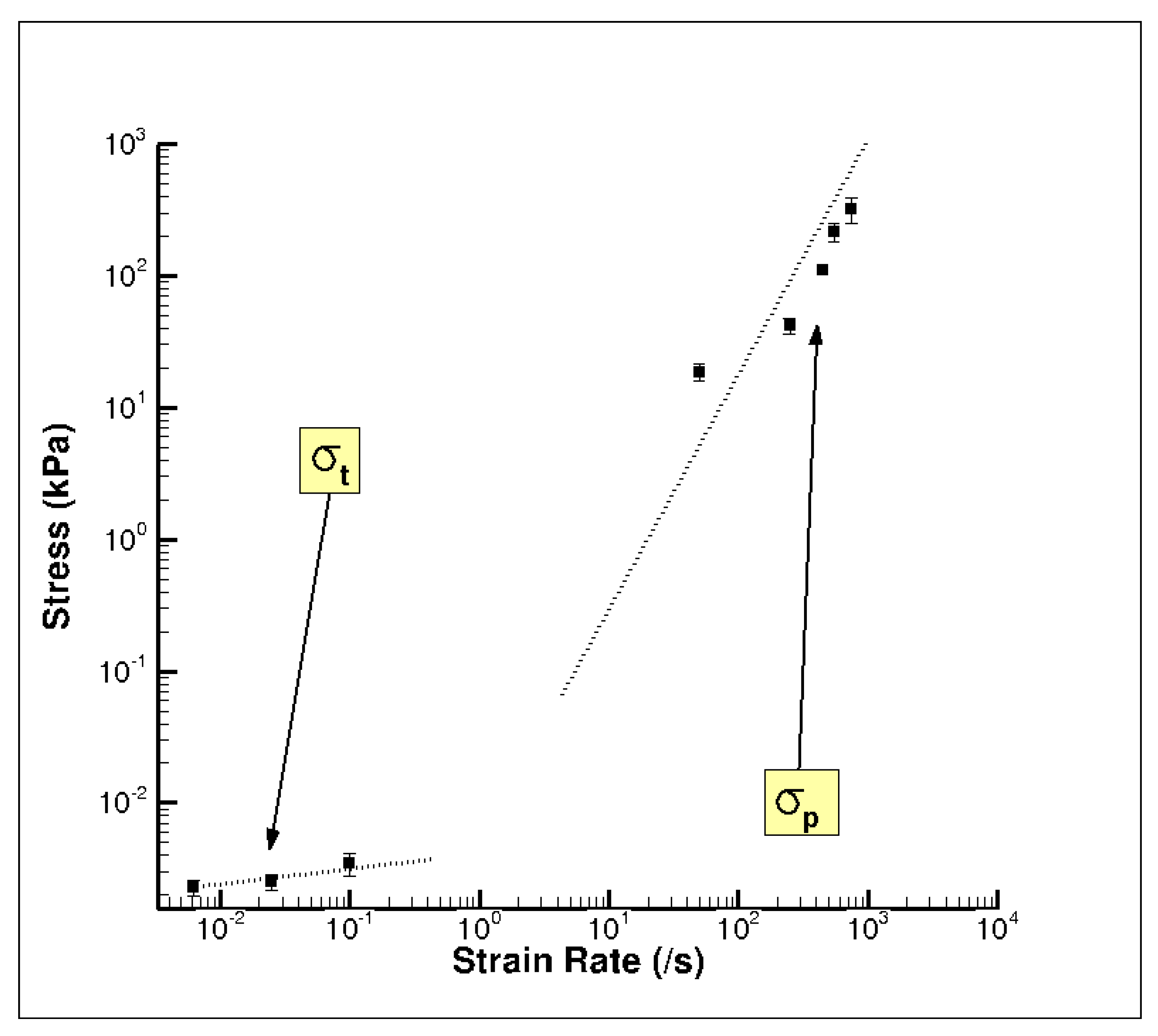
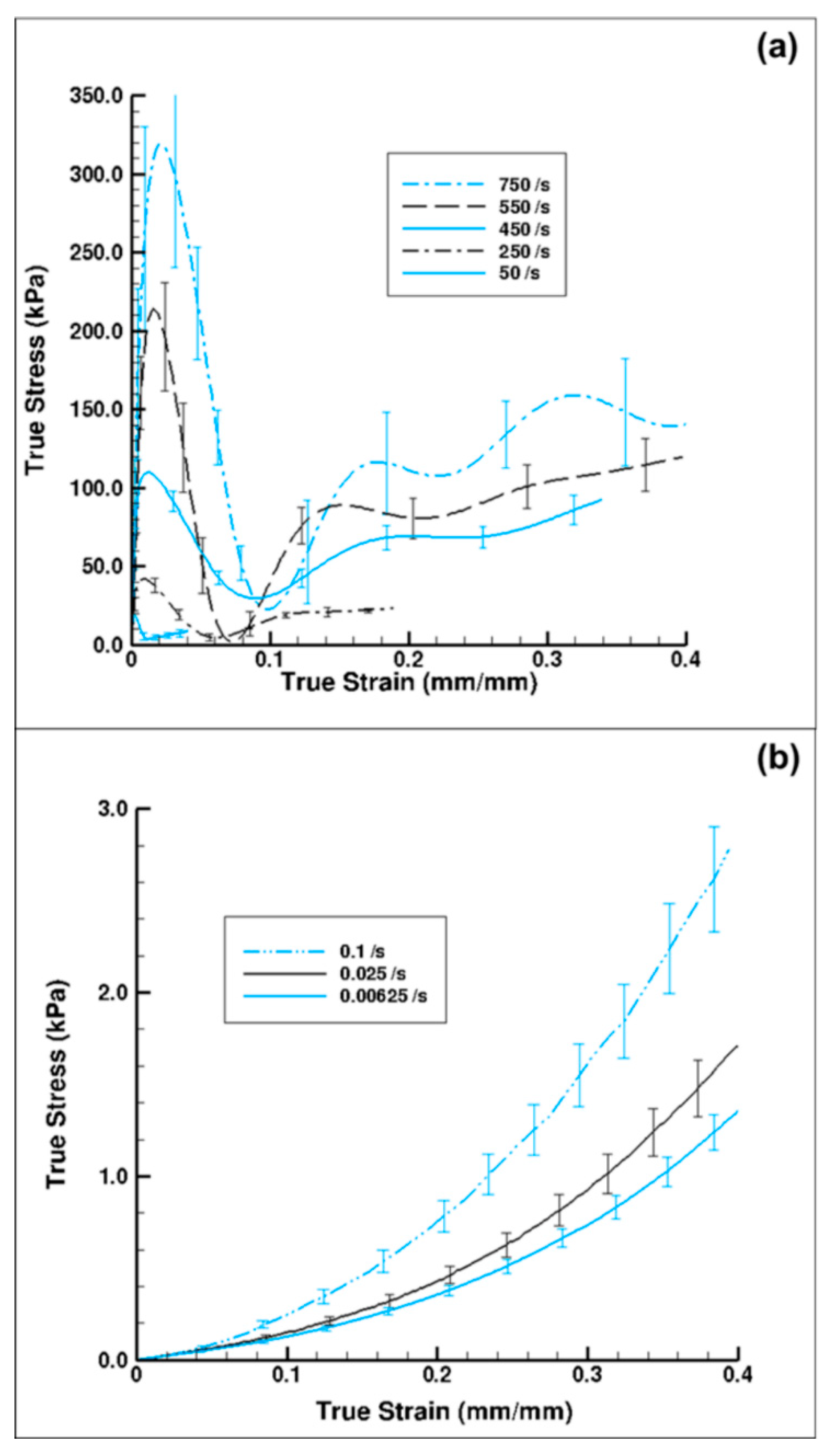
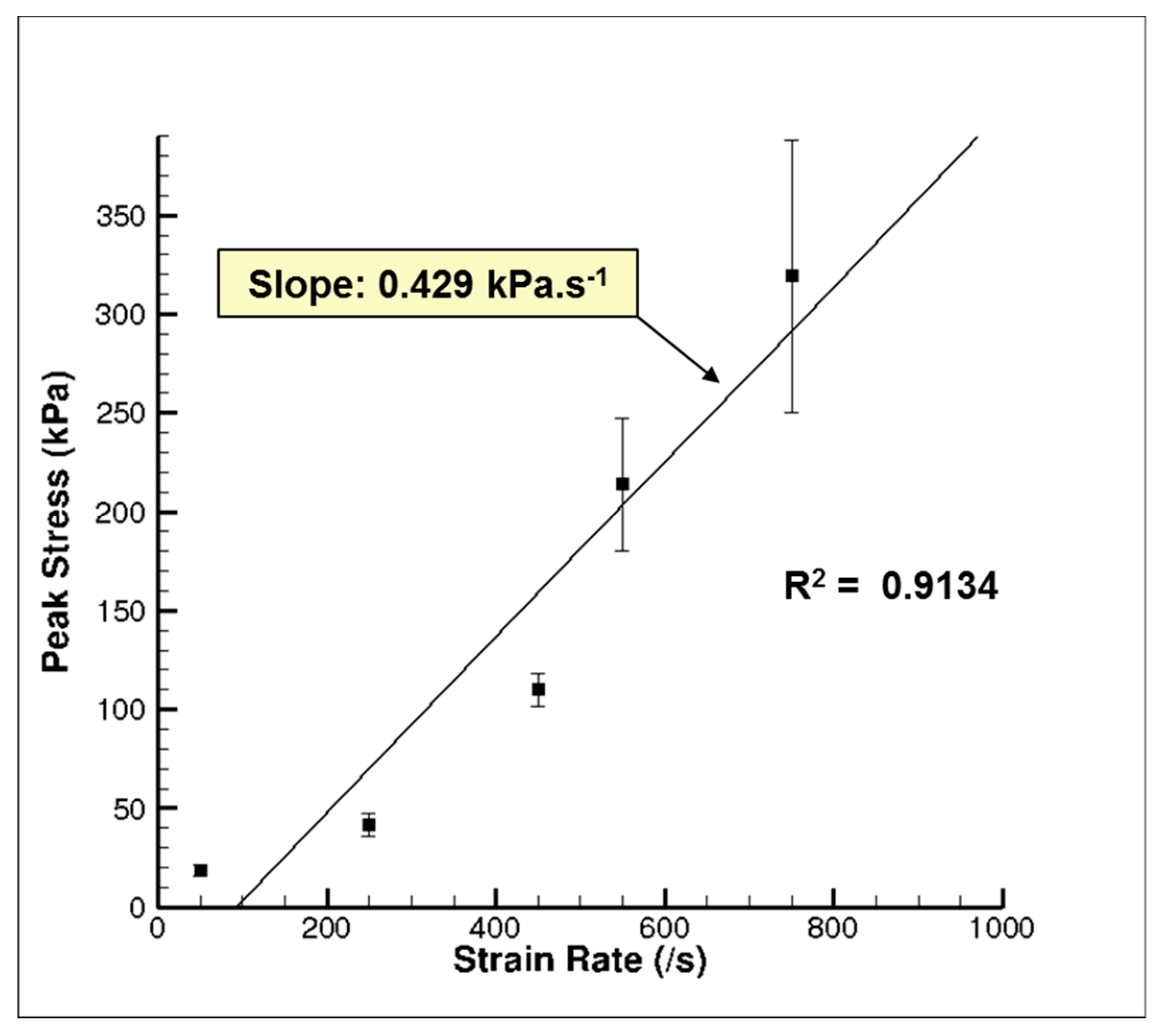
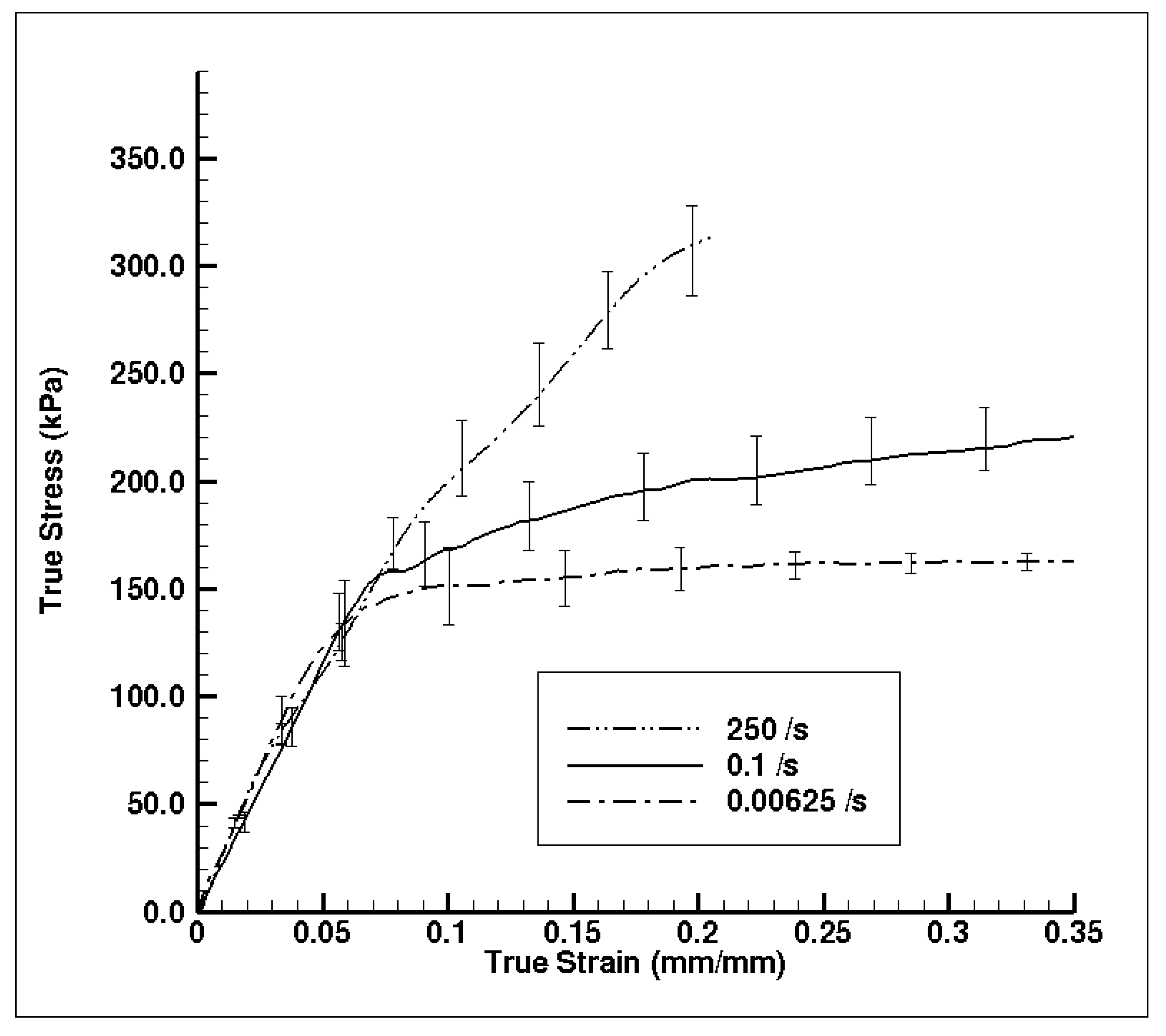
3.1. Experiment Response
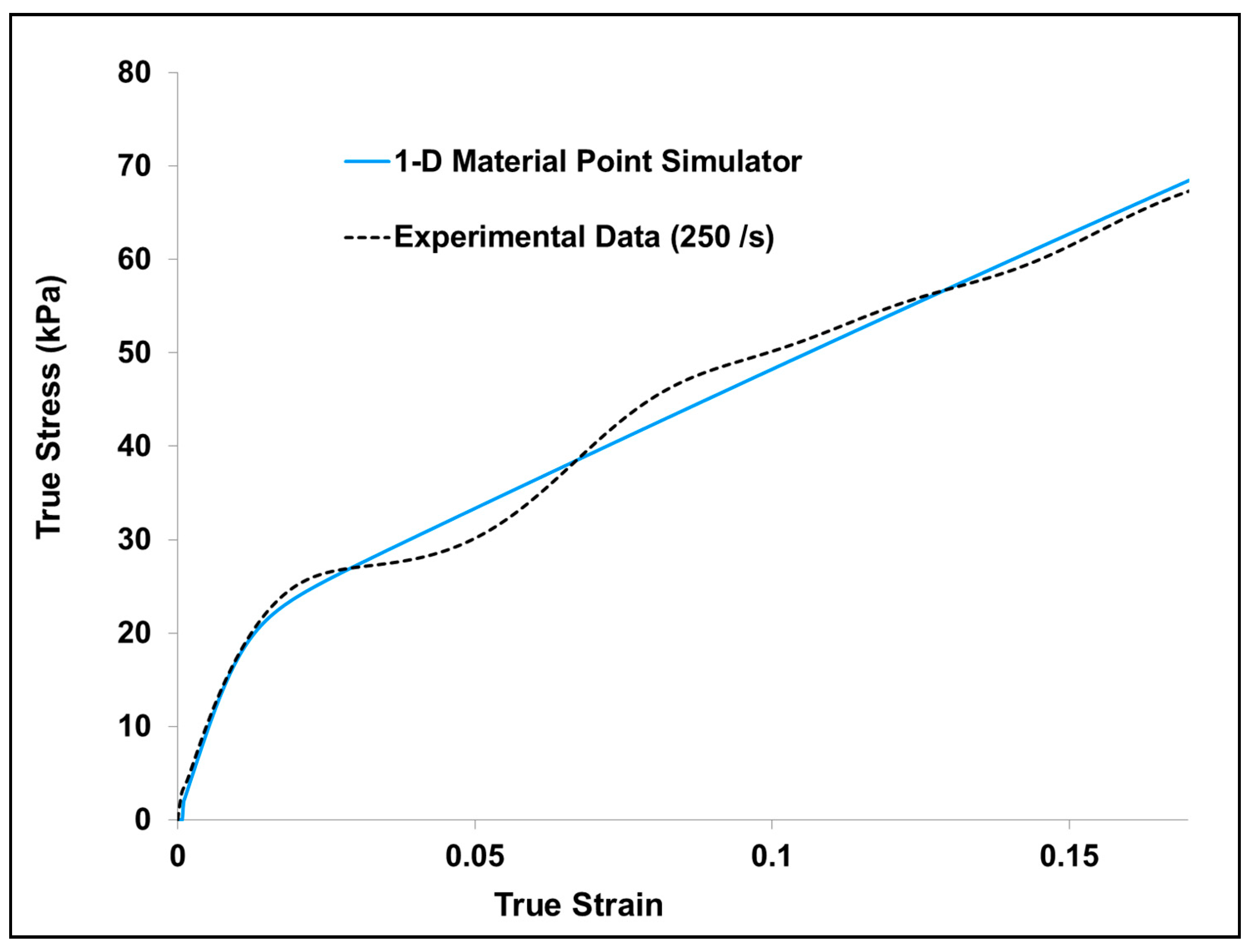
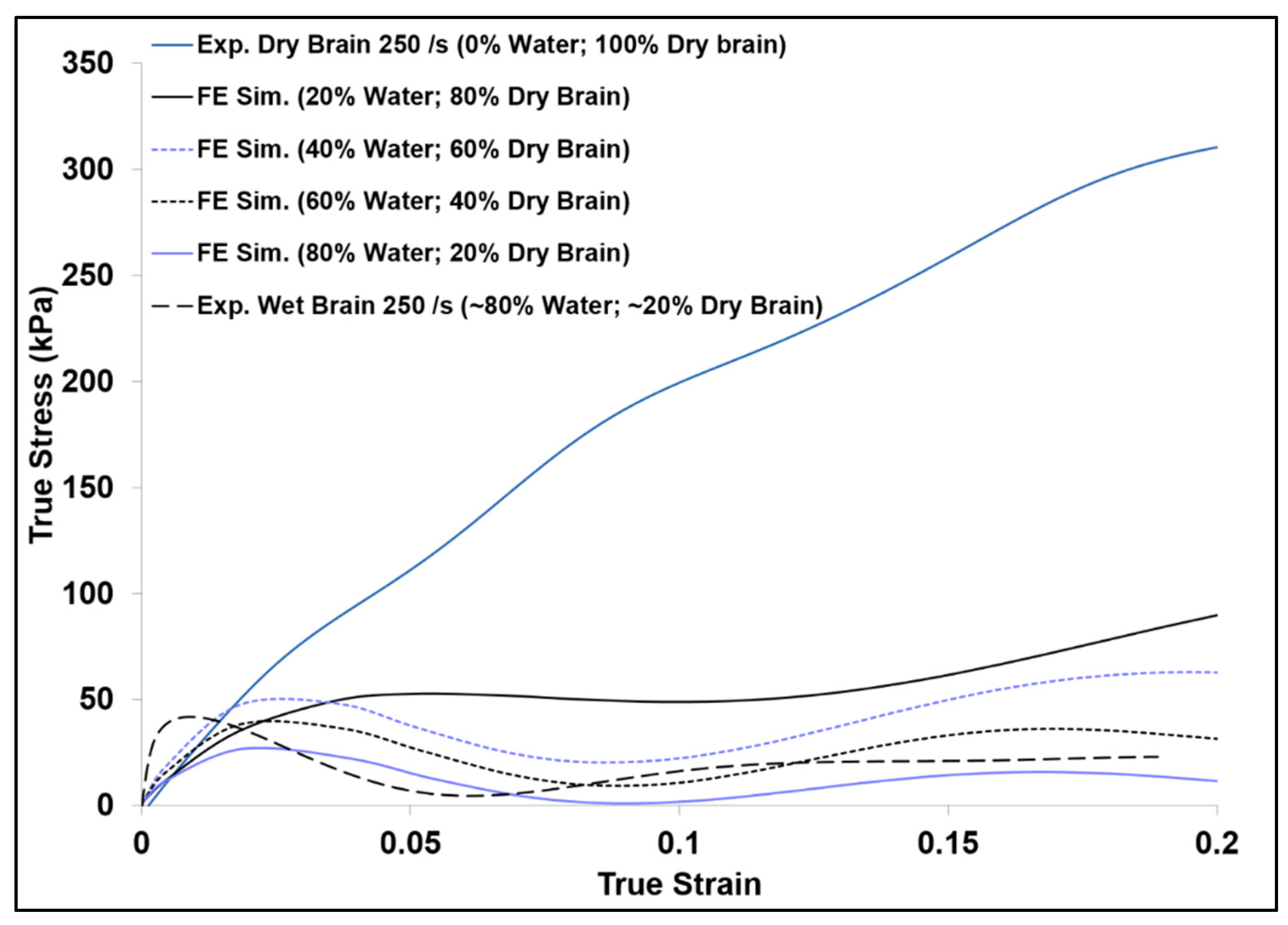
3.2. Simulation Response
4. Conclusions
Author Contributions
Funding
Acknowledgments
Conflicts of Interest
Appendix A
Appendix B

Appendix C

| Symbol | Description |
|---|---|
| Wave velocity | |
| Particle velocity | |
| , s | Wave velocity and particle velocity linear relationship constants |
| Free energy | |
| Rate of change of the strain energy density function | |
| Elastic part or the right Cauchy–Green tensor | |
| ,, | Internal strain fields (internal state variables) |
| Evolving strain threshold | |
| , | Saturation value of , |
| Cauchy stress | |
| F | Deformation gradient |
| , | Elastic part of F, transpose of the elastic part of F |
| , | Plastic part of F, transpose of the plastic part of F |
| Determinant of F, determinant of , Determinant of | |
| Elastic rate of deformation, inelastic rate of deformation | |
| Second Piola–Kirchoff stress | |
| Plastic rotational deformation | |
| Elastic portion of the rotation tensor, transpose of the elastic portion of the rotation tensor | |
| Right stretch tensor | |
| Mandel stress | |
| Kirchoff stress (elasto-viscoplastic part) | |
| Elastic shear moduli | |
| Identity matrix | |
| Elastic part of the Green–Lagrange strain | |
| Bulk moduli | |
| , | Stress-like thermodynamic conjugates to , |
| Stress-like thermodynamic conjugate to | |
| Viscous shear strain rate | |
| Reference viscous shear strain rate | |
| Effective pressure | |
| Equivalent shear stress | |
| αp | Stress-like thermodynamic conjugate of |
| Y | Yield criterion |
| Stretch tensor | |
| Rate of stretch tensor | |
| , , | Hardening moduli |
| Intermediate plastic configuration | |
| σt | Elastic-viscoelastic transition stress |
| σp | Elastic-plastic transition stress |
| Direction of viscous flow | |
| Hoppy bar velocities | |
| t | Time |
| Strain | |
| , | Hoppy bar sample strain rate, hoppy bar sample strain |
| Sample instantaneous length | |
| Hoppy bar areas | |
| Hoppy bar forces | |
| Hoppy bar elastic moduli | |
| Strain in the incident and transmitted hoppy bars | |
| Hoppy bar sample stress | |
| Hoppy bar sample area | |
| Engineering stress, engineering strain | |
| Initial sample area | |
| P | Force applied on the material |
| Current and reference lengths | |
| True stress, true strain |
References
- Langlois, J.A.; Rutland-Brown, W.; Wald, M.M. The Epidemiology and Impact of Traumatic Brain Injury A Brief Overview. J. Head Trauma Rehabilm 2006, 21, 375–378. [Google Scholar] [CrossRef]
- Finkelstein, E.A.; Corso, P.S.; Miller, T.R. The Incidence and Economic Burden of Injuries in the United States; Oxford University Press: New York, NY, USA, 2006; ISBN 9780195179484. [Google Scholar]
- Thurman, D.J.; Alverson, C.; Dunn, K.A.; Guerrero, J.; Sniezek, J.E. Traumatic Brain Injury in the United States: A Public Health Perspective. J. Head Trauma Rehabil. 1999, 14, 602–615. [Google Scholar] [CrossRef] [PubMed]
- Holbourn, A.H.S. MECHANICS OF HEAD INJURIES. Lancet 1943, 242, 438–441. [Google Scholar] [CrossRef]
- Pudenz, R.H.; Shelden, C.H. The Lucite Calvarium—A Method for Direct Observation of the Brain. J. Neurosurg. 1946, 3, 487–505. [Google Scholar] [CrossRef] [PubMed]
- Ommaya, A.K. Mechanical properties of tissues of the nervous system. J. Biomech. 1968, 1, 127–138. [Google Scholar] [CrossRef]
- Fallenstein, G.T.; Hulce, V.D.; Melvin, J.W. Dynamic mechanical properties of human brain tissue. J. Biomech. 1969, 2, 217–226. [Google Scholar] [CrossRef]
- Stalnaker, R.L. Mechanical Properties of the Head. West Virginia University, 1969. Available online: http://wbldb.lievers.net/10055045.html (accessed on 30 April 2019).
- Shuck, L.Z.; Advani, S.H. Rheological Response of Human Brain Tissue in Shear. J. Basic Eng. 1972, 94, 905–911. [Google Scholar] [CrossRef]
- McElhaney, J.H.; Melvin, J.W.; Roberts, V.L.; Portnoy, H.D. Dynamic Characteristics of the Tissues of the Head. In Perspectives in Biomedical Engineering; Kenedi, R.M., Ed.; Palgrave Macmillan UK: London, UK, 1973; pp. 215–222. ISBN 978-1-349-01604-4. [Google Scholar]
- Estes, M.S.; McElhaney, J. Response of Brain Tissue of Compressive Loading. In Proceedings of the American Society of Mechanical Engineers Biomechanical and Human Factors Conference, Washington, DC, USA, 31 May–3 June 1970. [Google Scholar]
- Donnelly, B.R.; Medige, L. Shear Properties of Human Brain Tissue. Trans. ASME, J. Biomech. Eng. 1997, 119, 423–432. [Google Scholar]
- Arbogast, K.B.; Meaney, D.F.; Thibault, L.E. Biomechanical Characterization of the Constitutive Relationship for the Brainstem. In SAE Technical Paper 952716, Proceeding of the 39th Stapp Car Crash Conference, 8–10 November; Society of Automotive Engineers: Warrendale, PA, USA, 1995. [Google Scholar]
- Arbogast, K.B.; Margulies, S.S. Regional Differences in Mechanical Properties of the Porcine Central Nervous System. SAE Trans. 1997, 106, 3807–3814. [Google Scholar]
- Arbogast, K.B.; Margulies, S.S. Material characterization of the brainstem from oscillatory shear tests. J. Biomech. 1998, 31, 801–807. [Google Scholar] [CrossRef]
- Prange, M.T.; Meaney, D.F.; Margulies, S.S. Directional properties of gray and white brain tissue undergoing large deformation. Adv. Bioeng. 1998, 39, 151–152. [Google Scholar]
- Aimedieu, P.; Grebe, R.; Idy-Peretti, I. Study of brain white matter anisotropy. Annu. Int. Conf. IEEE Eng. Med. Biol. 2001, 2, 1009–1011. [Google Scholar]
- Miller, K. How to test very soft biological tissues in extension? J. Biomech. 2001, 34, 651–657. [Google Scholar] [CrossRef]
- Miller, K.; Chinzei, K. Mechanical properties of brain tissue in tension. J. Biomech. 2002, 35, 483–490. [Google Scholar] [CrossRef]
- Bayly, P.V.; Black, E.E.; Pedersen, R.C.; Leister, E.P.; Genin, G.M. In vivo imaging of rapid deformation and strain in an animal model of traumatic brain injury. J. Biomech. 2006, 39, 1086–1095. [Google Scholar] [CrossRef] [PubMed]
- Smith, D.H.; Wolf, J.A.; Lusardi, T.A.; Lee, V.M.-Y.; Meaney, D.F. High Tolerance and Delayed Elastic Response of Cultured Axons to Dynamic Stretch Injury. J. Neurosci. 1999, 19, 4263–4269. [Google Scholar] [CrossRef] [PubMed]
- Tamura, A.; Hayashi, S.; Watanabe, I.; Nagayama, K.; Matsumoto, T. Mechanical Characterization of Brain Tissue in High-Rate Compression. J. Biomech. Sci. Eng. 2007, 2, 115–126. [Google Scholar] [CrossRef]
- Bain, A.C.; Meaney, D.F. Tissue-level thresholds for axonal damage in an experimental model of central nervous system white matter injury. J. Biomech. Eng. 2000, 122, 615–622. [Google Scholar] [CrossRef]
- Pfister, B.J.; Weihs, T.P.; Betenbaugh, M.; Bao, G. An in vitro uniaxial stretch model for axonal injury. Ann. Biomed. Eng. 2003, 31, 589–598. [Google Scholar] [CrossRef]
- Begonia, M.T.; Prabhu, R.; Liao, J.; Horstemeyer, M.F.; Williams, L.N. The Influence of Strain Rate Dependency on the Structure–Property Relations of Porcine Brain. Ann. Biomed. Eng. 2010, 38, 3043–3057. [Google Scholar] [CrossRef]
- Sparks, J.L.; Dupaix, R.B. Constitutive modeling of rate-dependent stress–strain behavior of human liver in blunt impact loading. Ann. Biomed. Eng. 2008, 36, 1883–1892. [Google Scholar] [CrossRef]
- Song, B.; Chen, W.; Ge, Y.; Weerasooriya, T. Dynamic and quasi-static compressive response of porcine muscle. J. Biomech. 2007, 40, 2999–3005. [Google Scholar] [CrossRef]
- Pervin, F.; Chen, W.W. Dynamic mechanical response of bovine gray matter and white matter brain tissues under compression. J. Biomech. 2009, 42, 731–735. [Google Scholar] [CrossRef]
- Prabhu, R.; Horstemeyer, M.F.; Tucker, M.T.; Marin, E.B.; Bouvard, J.L.; Sherburn, J.A.; Liao, J.; Williams, L.N. Coupled experiment/finite element analysis on the mechanical response of porcine brain under high strain rates. J. Mech. Behav. Biomed. Mater. 2011, 4, 1067–1080. [Google Scholar] [CrossRef]
- Clemmer, J.; Prabhu, R.; Chen, J.; Colebeck, E.; Priddy, L.B.; McCollum, M.; Brazile, B.; Whittington, W.; Wardlaw, J.L.; Rhee, H.; et al. Experimental Observation of High Strain Rate Responses of Porcine Brain, Liver, and Tendon. J. Mech. Med. Biol. 2016, 16, 1650032. [Google Scholar] [CrossRef]
- Cheng, S.; Bilston, L.E. Unconfined compression of white matter. J. Biomech. 2007, 40, 117–124. [Google Scholar] [CrossRef]
- Neeb, H.; Ermer, V.; Stocker, T.; Shah, N.J. Fast quantitative mapping of absolute water content with full brain coverage. Neuroimage 2008, 42, 1094–1109. [Google Scholar] [CrossRef]
- Hopkinson, B. The Effects of Momentary Stresses in Metals. Proc. R. Soc. London 1904, 74, 498–506. [Google Scholar] [CrossRef]
- Kolsky, H. An investigation of the mechanical properties of materials at very high rates of loading. Proc. R. Sot. Lond. B62 1949, 676, 676–700. [Google Scholar] [CrossRef]
- Tucker, M.T.; Horstemeyer, M.F.; Whittington, W.R.; Solanki, K.N.; Gullett, P.M. The effect of varying strain rates and stress states on the plasticity, damage, and fracture of aluminum alloys. Mech. Mater. 2010, 42, 895–907. [Google Scholar] [CrossRef]
- Gary, G.; Klepaczko, J.R.; Zhao, H. Generalization of split Hopkinson bar technique to use viscoelastic bars. Int. J. Impact Eng. 1995, 16, 529–530. [Google Scholar] [CrossRef]
- Prabhu, R.; Whittington, W.R.; Patnaik, S.S.; Mao, Y.; Begonia, M.T.; Williams, L.N.; Liao, J.; Horstemeyer, M.F. A Coupled Experiment-finite Element Modeling Methodology for Assessing High Strain Rate Mechanical Response of Soft Biomaterials. J. Vis. Exp. 2015, e51545. [Google Scholar] [CrossRef]
- Miller, K. Most recent results in the biomechanics of the brain. J. Biomech. 2005, 38, 965. [Google Scholar] [CrossRef] [PubMed]
- MacDonald, R.A.; MacDonald, W.M. Thermodynamic properties of fcc metals at high temperatures. Phys. Rev. B 1981, 24, 1715–1724. [Google Scholar] [CrossRef]
- Bouvard, J.L.; Ward, D.K.; Hossain, D.; Marin, E.B.; Bammann, D.J.; Horstemeyer, M.F. A general inelastic internal state variable model for amorphous glassy polymers. Acta Mech. 2010, 213, 71–96. [Google Scholar] [CrossRef]
- MATLAB 2010; The MathWorks Inc.: Natick, MA, USA, 2010.
- ABAQUS/Explicit User’s Manual 2009; Simulia Inc.: Providence, RI, USA, 2009.
- Franceschini, G.; Bigoni, D.; Regitnig, P.; Holzapfel, G.A. Brain tissue deforms similarly to filled elastomers and follows consolidation theory. J. Mech. Phys. Solids 2006, 54, 2592–2620. [Google Scholar] [CrossRef]
- Weinberg, K.; Ortiz, M. Shock wave induced damage in kidney tissue. Comput. Mater. Sci. 2005, 32, 588–593. [Google Scholar] [CrossRef]
- Ratajczak, M.; Ptak, M.; Chybowski, L.; Gawdzińska, K.; Bedziński, R. Material and structural modeling aspects of brain tissue deformation under dynamic loads. Materials (Basel) 2019, 12, 271. [Google Scholar] [CrossRef] [PubMed]
- Kaczyński, P.; Ptak, M.; Fernandes, F.A.O.; Chybowski, L.; Wilhelm, J.; de Sousa, R.J.A. Development and Testing of Advanced Cork Composite Sandwiches for Energy-Absorbing Structures. Materials (Basel) 2019, 12, 697. [Google Scholar] [CrossRef]
- Yamada, H.; Evans, F.G. Strength of Biological Materials; Williams & Wilkins: Philadelphia, PA, USA, 1970. [Google Scholar]
- Kroner, E. Allgemeine kontinuumstheorie der versetzungen und eigenspannungen. Arch. Ration. Mech. Anal. 1960, 4, 273–334. [Google Scholar] [CrossRef]
- Lee, E.H. Elastic plastic deformation at finite strain. ASME J. Appl. Mech. 1969, 36. [Google Scholar] [CrossRef]
- Gurtin, M.E.; Anand, L. The Decomposition F = FeFp, Material Symmetry, and Plastic Irrotationality for Solids that are Isotropic-Viscoplastic or Amorphous. Int. J. Plast. 2005, 21, 1686–1719. [Google Scholar] [CrossRef]
- Boyce, M.C.; Weber, G.G.; Parks, D.M. On the kinematics of finite strain plasticity. J. Mech. Phys. Solids 1989, 37, 647–665. [Google Scholar] [CrossRef]
- Fotheringham, D.G.; Cherry, B.W. Strain rate effects on the ratio of recoverable to non-recoverable strain in linear polyethylene. J. Mater. Sci. 1978, 13, 231–238. [Google Scholar] [CrossRef]
- Anand, L. Single-crystal elasto-viscoplasticity: Application to texture evolution in polycrystalline metals at large strains. Comput. Methods Appl. Mech. Eng. 2004, 193, 5359–5383. [Google Scholar] [CrossRef]
- Richeton, J.; Ahzi, S.; Vecchio, K.S.; Jiang, F.C.; Adharapurapu, R.R. Influence of temperature and strain rate on the mechanical behavior of three amorphous polymers: Characterization and modeling of the compressive yield stress. Int. J. Solids Struct. 2006, 43, 2318–2335. [Google Scholar] [CrossRef]
- Richeton, J.; Ahzi, S.; Vecchio, K.S.; Jiang, F.C.; Makradi, A. Modeling and validation of the large deformation inelastic response of amorphous polymers over a wide range of temperatures and strain rates. Int. J. Solids Struct. 2007, 44, 7938–7954. [Google Scholar] [CrossRef]
- Gent, A.N. A new constitutive relation for rubber. Rubber Chem. Technol. 1996, 69, 59–61. [Google Scholar] [CrossRef]
- Prantil, V.C.; Jenkins, J.T.; Dawson, P.R. An analysis of texture and plastic spin for planar polycrystals. J. Mech. Phys. Solids 1993, 41, 1357–1382. [Google Scholar] [CrossRef]
- Ames, N.M.; Srivastava, V.; Chester, S.A.; Anand, L. A thermo-mechanically coupled theory for large deformations of amorphous polymers. Part II: Applications. Int. J. Plast. 2009, 25, 1495–1539. [Google Scholar] [CrossRef]


| Strain Rate (s−1) | Wet/Dry | Number of Samples | Number of Animals/Porcine Brains | Temperature (°C) | Pressure (MPa) |
|---|---|---|---|---|---|
| 0.00625 | Wet | 6 | 3 | 20.85 | 0.1 |
| 0.025 | Wet | 7 | 4 | 20.85 | 0.1 |
| 0.1 | Wet | 16 | 7 | 20.85 | 0.1 |
| 50 | Wet | 6 | 3 | 20.85 | 0.1 |
| 250 | Wet | 4 | 2 | 20.85 | 0.1 |
| 450 | Wet | 5 | 2 | 20.85 | 0.1 |
| 550 | Wet | 7 | 3 | 20.85 | 0.1 |
| 750 | Wet | 4 | 2 | 20.85 | 0.1 |
| 0.00625 | Dry | 4 | 2 | 20.85 | 0.1 |
| 0.1 | Dry | 5 | 3 | 20.85 | 0.1 |
| 250 | Dry | 4 | 2 | 20.85 | 0.1 |
| Total | 68 | 33 |
| FE Simulation Case | Dry Brain % (m/m) | Water % (m/m) |
|---|---|---|
| 1 | 80 | 20 |
| 2 | 60 | 40 |
| 3 | 40 | 60 |
| 4 | 20 | 80 |
| Term/Function | Description |
|---|---|
| , where is the elastic part of the right Cauchy-Green tensor, and , and are internal strain fields (internal state variables). | Free energy, |
| , where Je-1 is the inverse of the determinant of . and are the elastic part of F and the transpose of elastic part of F. | Cauchy Stress, Second Piola-Kirchhoff Stress, |
| , where and are the elastic part of the rotation tensor (R) and the transpose of the elastic part of R. , where μ and K are the elastic shear and bulk moduli modeling the elastic behavior respectively. is the elastic part of the Green-Lagrange strain tensor, and is the identity matrix. , where is the plastic part of the deformation tensor, and is the right stretch tensor. | Kirchhoff Stress (elasto-viscoplastic part, ) Elastic Law (Mandel Stress, ) Deformation Gradient |
| , , where and are stress-like thermodynamic conjugates of the and respectively. , where is a stress-like thermodynamic conjugate of . | Stress-like internal state variables Stress-like internal state variable |
| , where is the inelastic rate of deformation. with , where is the viscous shear strain rate given by the following equation: with and , where is an equivalent shear stress term and is the effective pressure term, is a reference strain rate, m is a strain rate sensitivity parameter, and αp is a pressure sensitivity parameter and Y is the yield criterion. , , where represents an evolving strain threshold or criterion that the macromolecular chains must overcome to slip. h0 and g0 are hardening moduli, and is the saturation value of . with and where is the hardening modulus, and is the saturation value of ξ2. and | Flow rule Equivalent plastic shear strain-rate Polymer chain resistance to plastic flow Polymer chain crystallization at large strain Evolution equation of stretch-like tensor |
| Material constants |
| Model Constants | Constant Definition | Values |
|---|---|---|
| μ (MPa) | Shear Modulus | 0.80 |
| K (MPa) | Bulk Modulus | 399.73 |
| (s−1) | Reference Strain Rate | 120,000 |
| m | Strain Rate Sensitivity Parameter | 0.90 |
| Yo (MPa) | Material Yield Parameter | 9.00 |
| αp | Sensitivity Parameter | 0 |
| λL | Network Locking Stretch | 2.00 |
| μR | Rubbery Modulus | 0.07 |
| Rs1 | Material Hardening Parameter | 1.4 |
| ho | Hardening Modulus | 0.41 |
| ξo1 | Internal Strain-Like Parameter Initial Value | 0.0045 |
| ξ*sat | Internal Strain-Like Parameter Saturation Value | 0.001 |
| ξ*o | Energetic Strain Barrier | 1.2 |
| go | Hardening Modulus | 0.3 |
| Cκ1 (MPa) | Internal Stress-Like Parameter | 0.41 |
| h1 | Hardening Modulus | 0 |
| eos2 | Internal Strain-Like Parameter Initial Value | 0 |
| esats2 | Internal Strain-Like Parameter Saturation Value | 0.4 |
| Cκ2 (MPa) | Internal Stress-Like Parameter | 0 |
| Strain Rate (s−1) | 0.00625 s−1 n = 6 | 0.0250 s−1 n = 7 | 0.100 s−1 n = 16 | p-Value | |
|---|---|---|---|---|---|
| Variable | |||||
| Tangent Modulus (kPa) | 1.6822 ± 0.0047 | 1.7497 ± 0.0021 | 3.2378 ± 0.0371 | <0.05 | |
| Transition Stress (kPa) | 0.1046 ± 0.0046 | 0.1069 ± 0.0020 | 0.1400 ± 0.0377 | >0.05 | |
| Strain at Peak Stress | 0.075 ± 0.0040 | 0.075 ± 0.0060 | 0.072 ± 0.0050 | >0.05 | |
| Strain Rate (s−1) | 0.00625 s−1 n = 4 | 0.100 s−1 n = 5 | 250 s−1 n = 4 | p-Value | |
|---|---|---|---|---|---|
| Variable | |||||
| Tangent Modulus (kPa) | 2591.451 ± 424.4080 | 2282.160 ± 922.3810 | 2143.683 ± 620.0000 | >0.05 | |
| Transition Stress (kPa) | 108.602 ± 17.7860 | 138.313 ± 55.9020 | 166.389 ± 48.1420 | >0.05 | |
| Strain at Transition Stress | 0.0419 ± 0.0086 | 0.0606 ± 0.0100 | 0.0776 ± 0.0106 | >0.05 | |
© 2019 by the authors. Licensee MDPI, Basel, Switzerland. This article is an open access article distributed under the terms and conditions of the Creative Commons Attribution (CC BY) license (http://creativecommons.org/licenses/by/4.0/).
Share and Cite
Prabhu, R.K.; Begonia, M.T.; Whittington, W.R.; Murphy, M.A.; Mao, Y.; Liao, J.; Williams, L.N.; Horstemeyer, M.F.; Sheng, J. Compressive Mechanical Properties of Porcine Brain: Experimentation and Modeling of the Tissue Hydration Effects. Bioengineering 2019, 6, 40. https://doi.org/10.3390/bioengineering6020040
Prabhu RK, Begonia MT, Whittington WR, Murphy MA, Mao Y, Liao J, Williams LN, Horstemeyer MF, Sheng J. Compressive Mechanical Properties of Porcine Brain: Experimentation and Modeling of the Tissue Hydration Effects. Bioengineering. 2019; 6(2):40. https://doi.org/10.3390/bioengineering6020040
Chicago/Turabian StylePrabhu, Raj K., Mark T. Begonia, Wilburn R. Whittington, Michael A. Murphy, Yuxiong Mao, Jun Liao, Lakiesha N. Williams, Mark F. Horstemeyer, and Jianping Sheng. 2019. "Compressive Mechanical Properties of Porcine Brain: Experimentation and Modeling of the Tissue Hydration Effects" Bioengineering 6, no. 2: 40. https://doi.org/10.3390/bioengineering6020040
APA StylePrabhu, R. K., Begonia, M. T., Whittington, W. R., Murphy, M. A., Mao, Y., Liao, J., Williams, L. N., Horstemeyer, M. F., & Sheng, J. (2019). Compressive Mechanical Properties of Porcine Brain: Experimentation and Modeling of the Tissue Hydration Effects. Bioengineering, 6(2), 40. https://doi.org/10.3390/bioengineering6020040