

Enhancing Knee MR Image Clarity through Image Domain Super-Resolution Reconstruction


Abstract
1. Introduction
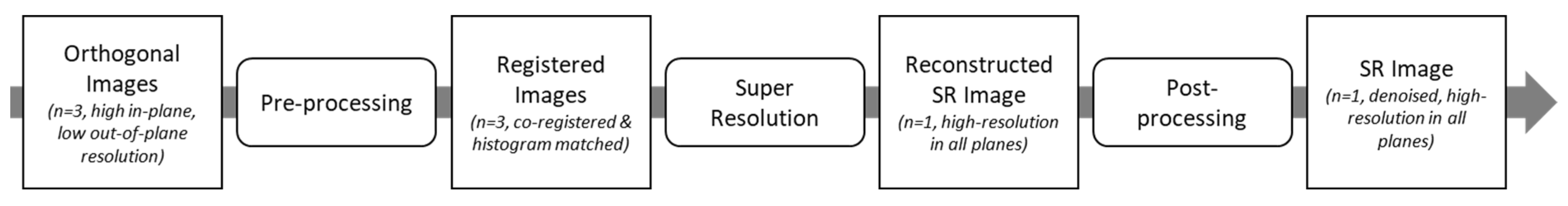
2. Methods
2.1. Preprocessing
2.2. Super-Resolution
2.3. Post-Processing—Artefact Reduction Convolutional Neural Network
2.4. Evaluation of Methods
3. Results
4. Discussion
5. Conclusions
Author Contributions
Funding
Institutional Review Board Statement
Informed Consent Statement
Data Availability Statement
Conflicts of Interest
Appendix A
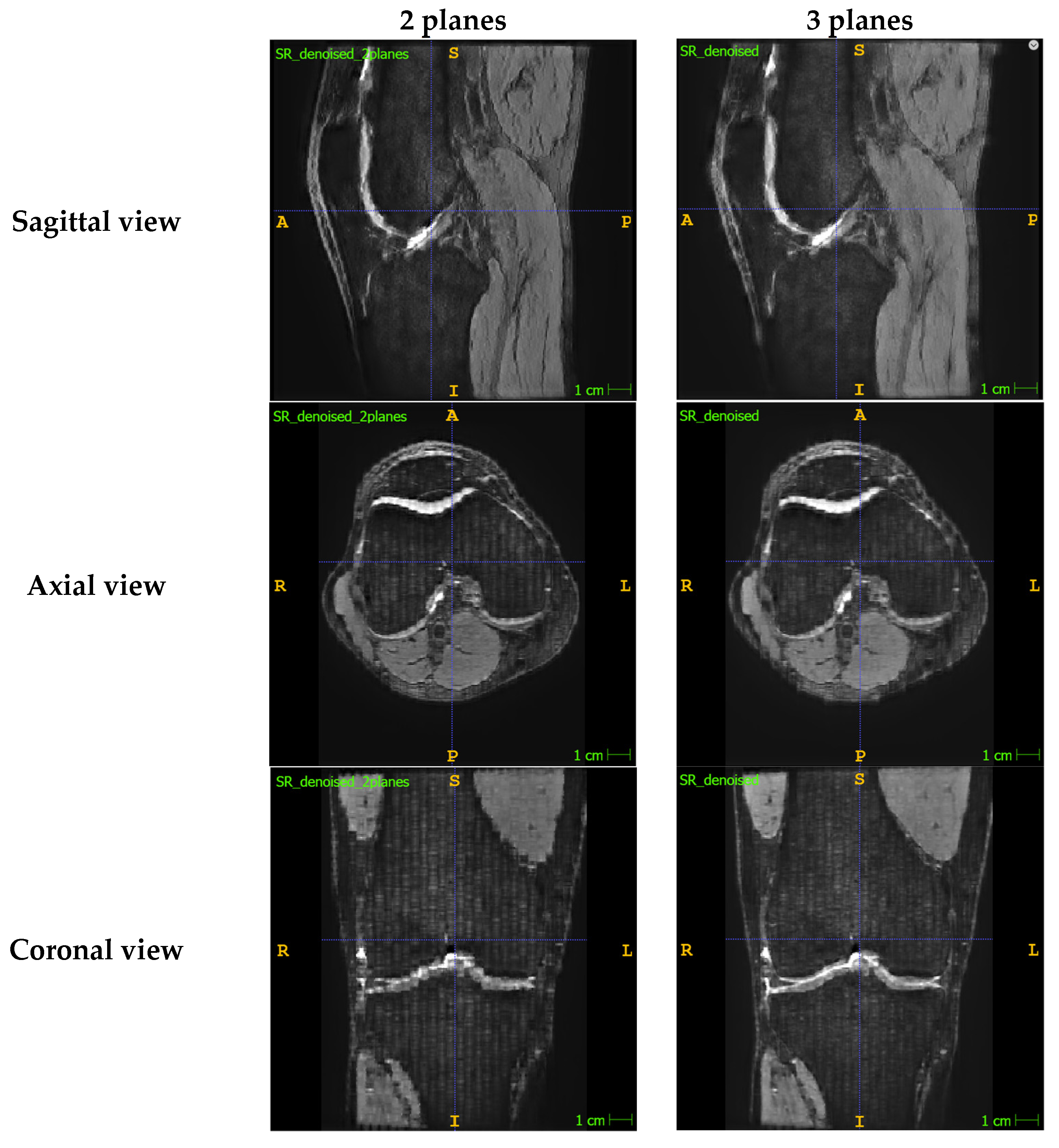
Appendix A.1. Presenting the Comparison between SR Images Reconstructed with Two Planes vs. Three Planes
Appendix A.2. Summary of the 3D Slicer Registration Parameters

| Input Images | |
|---|---|
| Fixed image volume | Isotropic sagittal image |
| Moving image volume | Axial image OR coronal image |
| Percentage of samples | 0.002 |
| B-spline grid size | 14,10,12 |
| Output settings | |
| Slicer linear transform | None |
| Slicer Bspline transform | None |
| Output image volume | Registered axial image OR Registered coronal image |
| Transform initialisation settings | |
| Initialisation transform | None |
| Initialise transform mode | Off |
| Registration phases | Rigid and affine selected |
| Image Mask and Pre-processing | Default settings |
| Advanced output settings | |
| Fixed image volume 2 | None |
| Moving image volume 2 | None |
| Output image pixel type | Float |
| Background fill value | 0.0 |
| Interpolation mode | Linear |
| Advanced optimisation settings | |
| Max iterations | 1500 |
| Maximum step length | 0.05 |
| Minimum step length | 0.001 |
| Relaxation factor | 0.5 |
| Transform scale | 1000.0 |
| Reproportion scale | 1.0 |
| Skew scale | 1.0 |
| Maximum B-spline displacement | 0.0 |
| Expert-only parameters | |
| Fixed image time index | 0 |
| Moving image time index | 0 |
| Histogram bin count | 50 |
| Histogram match point count | 10 |
| Cost metric | NC (i.e., normalised correlation) |
| Inferior cut off from centre | 1000.0 |
| ROIAuto dilate size | 0.0 |
| ROIAuto closing size | 9.0 |
| Number of samples | 0 |
| Stripped output transform | None |
| Output transform | None |
| Debugging parameters | Default settings |
Appendix A.3. Worked Example Showing How the Intensity Value Is Calculated for a Template Voxel
| Image Stack | Distance from Template Voxel (mm) | Intensity Value |
|---|---|---|
| Sagittal | 2 | 173 |
| Axial | 3 | 198 |
| Coronal | 5 | 127 |
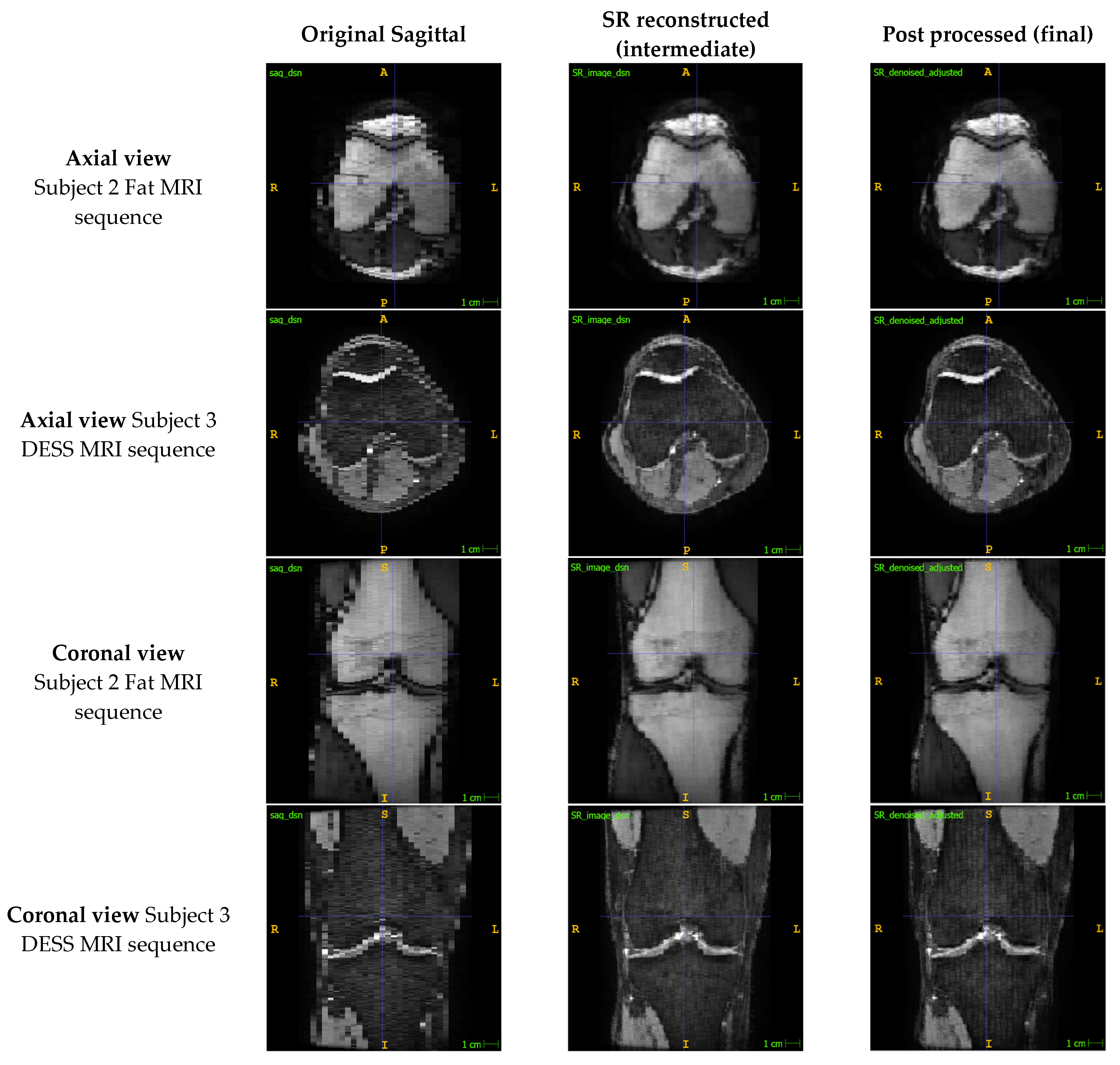
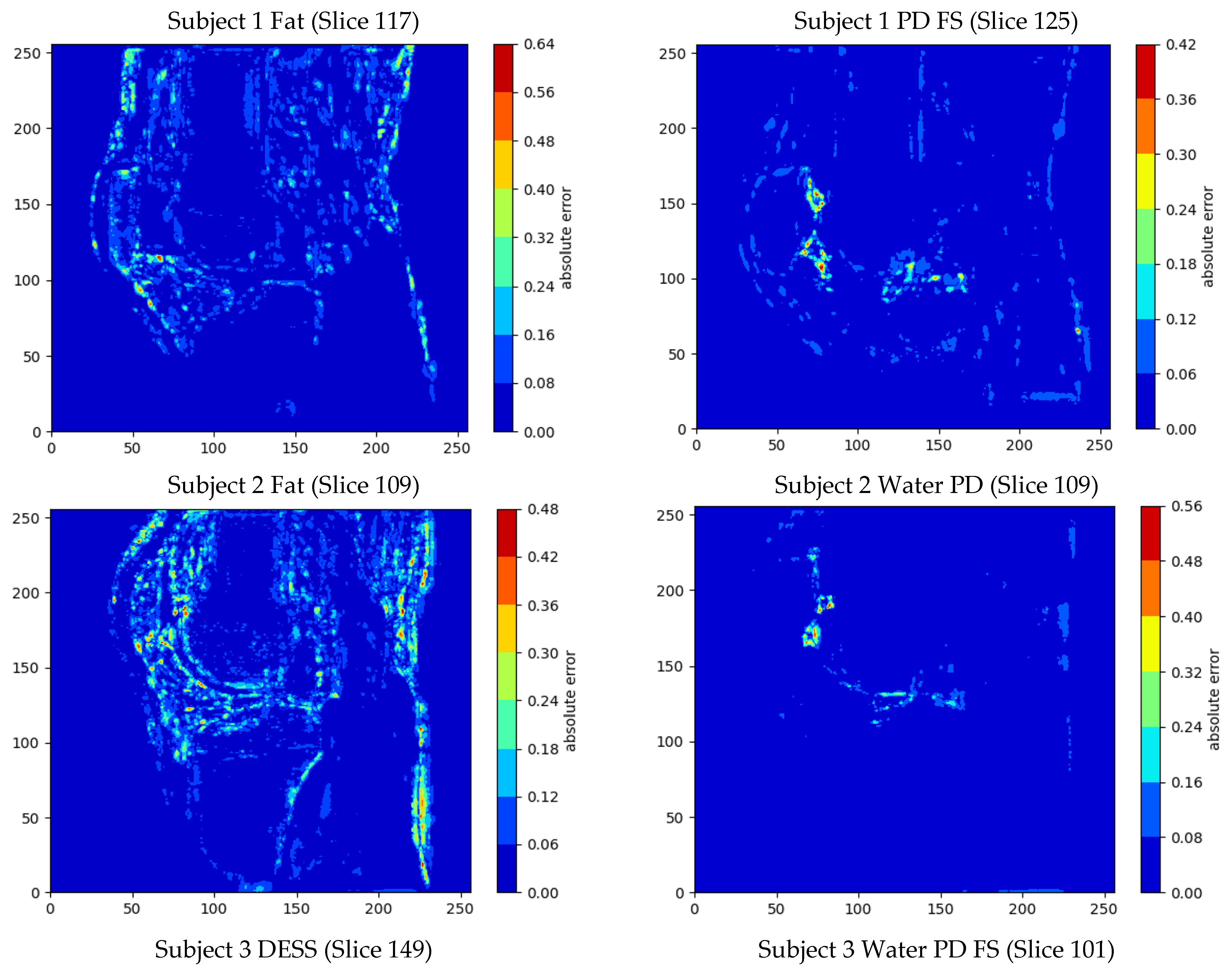
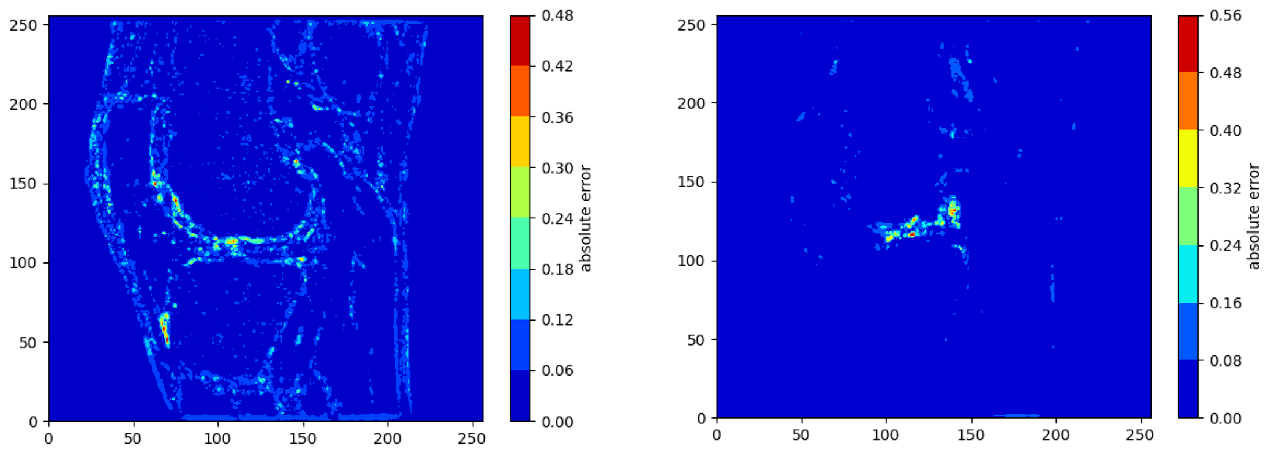
Appendix A.4. Presenting the Quantitative Analysis Results between the Intermediate SR Reconstructed Image and the Original High-Resolution MR Image
| Subject (MR Sequence) | MSE | Mean Error ± Standard Deviation | PSNR (dB) | SSIM | Max Error | Min Error |
|---|---|---|---|---|---|---|
| 1 (Fat) | 0.091% | 1.36% ± 2.70% | 30.40 | 0.939 | 58.8% | 0% |
| 1 (PD FS) | 0.013% | 0.50% ± 1.03% | 38.80 | 0.966 | 62.6% | 0% |
| 2 (Fat) | 0.103% | 1.47% ± 2.86% | 29.86 | 0.926 | 64.8% | 0% |
| 2 (Water PD) | 0.019% | 0.76% ± 1.15% | 37.20 | 0.965 | 61.3% | 0% |
| 3 (DESS) | 0.058% | 1.14% ± 2.12% | 32.36 | 0.888 | 77.3% | 0% |
| 3 (Water PD FS) | 0.027% | 0.85% ± 1.39% | 35.76 | 0.966 | 60.4% | 0% |
| Mean | 0.052% | 1.01% ± 1.88% | 34.06 | 0.942 | 64.2% | 0% |
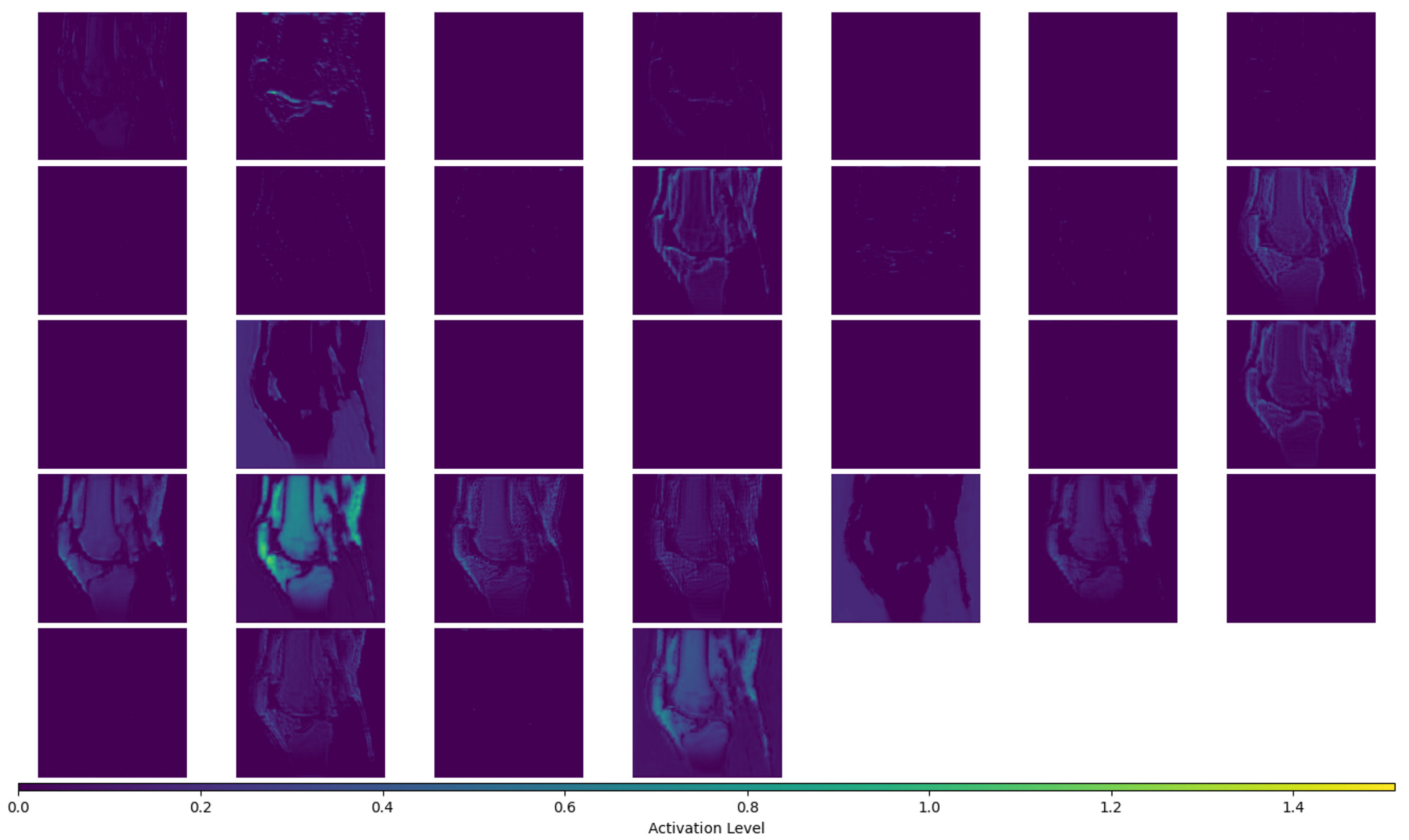
Appendix A.5. Presenting the Activation Maps for the “Feature Enhancement” Layer of the ARCNN for a Single Slice of One of the High-Resolution MR Images
References
- Gholipour, A.; Afacan, O.; Aganj, I.; Scherrer, B.; Prabhu, S.P.; Sahin, M.; Warfield, S.K. Super-Resolution Reconstruction in Frequency, Image, and Wavelet Domains to Reduce through-Plane Partial Voluming in MRI. Med. Phys. 2015, 42, 6919–6932. [Google Scholar] [CrossRef]
- Woo, J.; Murano, E.Z.; Stone, M.; Prince, J.L. Reconstruction of High-Resolution Tongue Volumes from MRI. IEEE Trans. Biomed. Eng. 2012, 59, 3511–3524. [Google Scholar] [CrossRef]
- Plenge, E.; Poot, D.H.J.; Bernsen, M.; Kotek, G.; Houston, G.; Wielopolski, P.; Van Der Weerd, L.; Niessen, W.J.; Meijering, E. Super-Resolution in MRI: Better Images Faster? Haynor, D.R., Ourselin, S., Eds.; Proceedings of SPIE: San Diego, CA, USA, 2012; p. 83143V. [Google Scholar]
- Grover, V.P.B.; Tognarelli, J.M.; Crossey, M.M.E.; Cox, I.J.; Taylor-Robinson, S.D.; McPhail, M.J.W. Magnetic Resonance Imaging: Principles and Techniques: Lessons for Clinicians. J. Clin. Exp. Hepatol. 2015, 5, 246–255. [Google Scholar] [CrossRef] [PubMed]
- Van Reeth, E.; Tham, I.W.K.; Tan, C.H.; Poh, C.L. Super-Resolution in Magnetic Resonance Imaging: A Review. Concepts Magn. Reson. Part A 2012, 40A, 306–325. [Google Scholar] [CrossRef]
- Plenge, E.; Poot, D.H.J.; Bernsen, M.; Kotek, G.; Houston, G.; Wielopolski, P.; van der Weerd, L.; Niessen, W.J.; Meijering, E. Super-Resolution Methods in MRI: Can They Improve the Trade-off between Resolution, Signal-to-Noise Ratio, and Acquisition Time? Magn. Reson. Med. 2012, 68, 1983–1993. [Google Scholar] [CrossRef]
- Greenspan, H.; Oz, G.; Kiryati, N.; Peled, S. MRI Inter-Slice Reconstruction Using Super-Resolution. Magn. Reson. Imaging 2002, 20, 437–446. [Google Scholar] [CrossRef]
- Yan, Z.; Lu, Y. Super Resolution of MRI Using Improved IBP. In Proceedings of the 2009 International Conference on Computational Intelligence and Security, Beijing, China, 11–14 December 2009; pp. 643–647. [Google Scholar] [CrossRef]
- Souza, A.; Senn, R. Model-Based Super-Resolution for MRI. In Proceedings of the 2008 30th Annual International Conference of the IEEE Engineering in Medicine and Biology Society, Vancouver, BC, Canada, 20–25 August 2008; pp. 430–434. [Google Scholar] [CrossRef]
- Bai, Y.; Han, X.; Prince, J.L. Super-Resolution Reconstruction of MR Brain Images. In Proceedings of the 38th Annual Conference on Information Sciences and Systems (CISS04); 2004. [Google Scholar]
- Lu, Y.; Yang, R.; Zhang, J.; Zhang, C. Super Resolution Image Reconstruction in Parallel Magnetic Resonance Imaging. In Proceedings of the IEEE ICCA 2010, Xiamen, China, 9–11 June 2010; pp. 761–766. [Google Scholar]
- Shilling, R.Z.; Robbie, T.Q.; Bailloeul, T.; Mewes, K.; Mersereau, R.M.; Brummer, M.E. A Super-Resolution Framework for 3-D High-Resolution and High-Contrast Imaging Using 2-D Multislice MRI. IEEE Trans. Med. Imaging 2009, 28, 633–644. [Google Scholar] [CrossRef]
- Goshtasby, A.A.; Turner, D.A. Fusion of Short-Axis and Long-Axis Cardiac MR Images. Comput. Med. Imaging Graph. Off. J. Comput. Med. Imaging Soc. 1996, 20, 77–87. [Google Scholar] [CrossRef]
- Steines, D.; Timsari, B.; Tsougarakis, K. Fusion of Multiple Imaging Planes for Isotropic Imaging in MRI and Quantitative Image Analysis Using Isotropic or Near-Isotropic Imaging 2012. US8094900B2, 10 January 2012. [Google Scholar]
- Kim, K.; Habas, P.A.; Rousseau, F.; Glenn, O.A.; Barkovich, A.J.; Studholme, C. Intersection Based Motion Correction of Multislice MRI for 3-D in Utero Fetal Brain Image Formation. IEEE Trans. Med. Imaging 2010, 29, 146–158. [Google Scholar] [CrossRef]
- Mahmoudzadeh, A.P.; Kashou, N.H. Interpolation-Based Super-Resolution Reconstruction: Effects of Slice Thickness. J. Med. Imaging 2014, 1, 034007. [Google Scholar] [CrossRef] [PubMed]
- Kashou, N.H.; Smith, M.A.; Roberts, C.J. Ameliorating Slice Gaps in Multislice Magnetic Resonance Images: An Interpolation Scheme. Int. J. Comput. Assist. Radiol. Surg. 2015, 10, 19–33. [Google Scholar] [CrossRef]
- Qiu, D.; Zhang, S.; Liu, Y.; Zhu, J.; Zheng, L. Super-Resolution Reconstruction of Knee Magnetic Resonance Imaging Based on Deep Learning. Comput. Methods Programs Biomed. 2020, 187, 105059. [Google Scholar] [CrossRef]
- Dong, C.; Loy, C.C.; He, K.; Tang, X. Image Super-Resolution Using Deep Convolutional Networks. IEEE Trans. Pattern Anal. Mach. Intell. 2016, 38, 295–307. [Google Scholar] [CrossRef]
- Chaudhari, A.S.; Fang, Z.; Kogan, F.; Wood, J.; Stevens, K.J.; Gibbons, E.K.; Lee, J.H.; Gold, G.E.; Hargreaves, B.A. Super-Resolution Musculoskeletal MRI Using Deep Learning. Magn. Reson. Med. 2018, 80, 2139–2154. [Google Scholar] [CrossRef] [PubMed]
- Andrew, J.; Mhatesh, T.S.R.; Sebastin, R.D.; Sagayam, K.M.; Eunice, J.; Pomplun, M.; Dang, H. Super-Resolution Reconstruction of Brain Magnetic Resonance Images via Lightweight Autoencoder. Inform. Med. Unlocked 2021, 26, 100713. [Google Scholar] [CrossRef]
- Zhao, C.; Shao, M.; Carass, A.; Li, H.; Dewey, B.E.; Ellingsen, L.M.; Woo, J.; Guttman, M.A.; Blitz, A.M.; Stone, M.; et al. Applications of a Deep Learning Method for Anti-Aliasing and Super-Resolution in MRI. Magn. Reson. Imaging 2019, 64, 132–141. [Google Scholar] [CrossRef]
- Dyrby, T.B.; Lundell, H.; Burke, M.W.; Reislev, N.L.; Paulson, O.B.; Ptito, M.; Siebner, H.R. Interpolation of Diffusion Weighted Imaging Datasets. NeuroImage 2014, 103, 202–213. [Google Scholar] [CrossRef] [PubMed]
- Zhou, F.; Yang, W.; Liao, Q. Interpolation-Based Image Super-Resolution Using Multisurface Fitting. IEEE Trans. Image Process. 2012, 21, 3312–3318. [Google Scholar] [CrossRef]
- Yu, K.; Dong, C.; Loy, C.C.; Tang, X. Deep Convolution Networks for Compression Artifacts Reduction 2016. arXiv 2016, arXiv:1608.02778. [Google Scholar]
- Xie, S.; Zheng, X.; Chen, Y.; Xie, L.; Liu, J.; Zhang, Y.; Yan, J.; Zhu, H.; Hu, Y. Artifact Removal Using Improved GoogLeNet for Sparse-View CT Reconstruction. Sci. Rep. 2018, 8, 6700. [Google Scholar] [CrossRef]
- Yeh, C.-H.; Lin, C.-H.; Lin, M.-H.; Kang, L.-W.; Huang, C.-H.; Chen, M.-J. Deep Learning-Based Compressed Image Artifacts Reduction Based on Multi-Scale Image Fusion. Inf. Fusion 2021, 67, 195–207. [Google Scholar] [CrossRef]
- Cui, L.; Song, Y.; Wang, Y.; Wang, R.; Wu, D.; Xie, H.; Li, J.; Yang, G. Motion Artifact Reduction for Magnetic Resonance Imaging with Deep Learning and K-Space Analysis. PLoS ONE 2023, 18, e0278668. [Google Scholar] [CrossRef] [PubMed]
- Johnson, H.; Harris, G.; Williams, K. BRAINSFIT: Mutual Information Registrations of Whole-Brain 3D Images, Using the Insight Toolkit. Insight J. 2007, 57, 1–10. [Google Scholar] [CrossRef]
- Registration—3D Slicer Documentation. Available online: https://slicer.readthedocs.io/en/latest/user_guide/registration.html (accessed on 24 November 2023).
- Wang, Z.; Bovik, A.C.; Sheikh, H.R.; Simoncelli, E.P. Image Quality Assessment: From Error Visibility to Structural Similarity. IEEE Trans. Image Process. 2004, 13, 600–612. [Google Scholar] [CrossRef]

| Layer | Type | Filters (i.e., Number of Output Channels) | Kernel (i.e., Size of the Convolution Filter) | Stride | Padding | Activation |
|---|---|---|---|---|---|---|
| (i) Feature extraction | Conv2D | 64 | 9 × 9 | 1 | Zero padding | ReLU |
| (ii) Shrinking | Conv2D | 32 | 1 × 1 | 1 | No padding | ReLU |
| (iii) Feature enhancement | Conv2D | 32 | 7 × 7 | 1 | Zero padding | ReLU |
| (iv) Mapping | Conv2D | 64 | 1 × 1 | 1 | No padding | ReLU |
| (v) Reconstruction | Conv2D Transpose | 1 | 7 × 7 | 1 | Zero padding | None |
| Index | Subject ID | Sequence | MRI Dimensions |
|---|---|---|---|
| 1 | 1 | Fat | 512 × 512 × 208 |
| 2 | 1 | PD FS | 512 × 512 × 228 |
| 3 | 2 | Fat | 512 × 512 × 208 |
| 4 | 2 | Water PD | 512 × 512 × 208 |
| 5 | 3 | DESS | 512 × 512 × 236 |
| 6 | 3 | Water PD FS | 512 × 512 × 188 |
| Subject (MR Sequence) | MSE | Mean Error ± Standard Deviation | PSNR (dB) | SSIM | Max Error | Min Error |
|---|---|---|---|---|---|---|
| 1 (Fat) | 0.123% | 1.75% ± 3.04% | 29.11 | 0.897 | 72.4% | 0% |
| 1 (PD FS) | 0.043% | 1.24% ± 1.68% | 33.62 | 0.880 | 71.4% | 0% |
| 2 (Fat) | 0.130% | 1.89% ± 3.07% | 28.85 | 0.870 | 70.0% | 0% |
| 2 (Water PD) | 0.037% | 1.12% ± 1.57% | 34.29 | 0.904 | 62.5% | 0% |
| 3 (DESS) | 0.074% | 1.42% ± 2.33% | 31.29 | 0.843 | 79.3% | 0% |
| 3 (Water PD FS) | 0.035% | 0.95% ± 1.63% | 34.50 | 0.919 | 68.5% | 0% |
| Mean | 0.074% | 1.40% ± 2.22% | 31.94 | 0.886 | 70.7% | 0% |
| Subject (MR Sequence) | Initialising coordinate Lists (s) | Binary Tree Creation and Finding Nearest Voxels and Their Distances (s) | Reconstruction (s) | Total Time (s) |
|---|---|---|---|---|
| 1 (Fat) | 633 | 1609 | 464 | 2706 |
| 1 (PD FS) | 846 | 2355 | 467 | 3668 |
| 2 (Fat) | 704 | 1519 | 340 | 2563 |
| 2 (Water PD) | 592 | 1487 | 311 | 2390 |
| 3 (DESS) | 842 | 1795 | 372 | 3009 |
| 3 (Water PD FS) | 532 | 1188 | 290 | 2010 |
| Mean | 692 | 1659 | 374 | 2725 |
| Standard deviation | 131 | 394 | 76 | 569 |
| % of total time | 25.4% | 60.9% | 13.7% | 100% |
| Time complexity | O(N) | O(Nlog(N)) | O(N) | - |
Disclaimer/Publisher’s Note: The statements, opinions and data contained in all publications are solely those of the individual author(s) and contributor(s) and not of MDPI and/or the editor(s). MDPI and/or the editor(s) disclaim responsibility for any injury to people or property resulting from any ideas, methods, instructions or products referred to in the content. |
© 2024 by the authors. Licensee MDPI, Basel, Switzerland. This article is an open access article distributed under the terms and conditions of the Creative Commons Attribution (CC BY) license (https://creativecommons.org/licenses/by/4.0/).
Share and Cite
Patel, V.; Wang, A.; Monk, A.P.; Schneider, M.T.-Y. Enhancing Knee MR Image Clarity through Image Domain Super-Resolution Reconstruction. Bioengineering 2024, 11, 186. https://doi.org/10.3390/bioengineering11020186
Patel V, Wang A, Monk AP, Schneider MT-Y. Enhancing Knee MR Image Clarity through Image Domain Super-Resolution Reconstruction. Bioengineering. 2024; 11(2):186. https://doi.org/10.3390/bioengineering11020186
Chicago/Turabian StylePatel, Vishal, Alan Wang, Andrew Paul Monk, and Marco Tien-Yueh Schneider. 2024. "Enhancing Knee MR Image Clarity through Image Domain Super-Resolution Reconstruction" Bioengineering 11, no. 2: 186. https://doi.org/10.3390/bioengineering11020186
APA StylePatel, V., Wang, A., Monk, A. P., & Schneider, M. T.-Y. (2024). Enhancing Knee MR Image Clarity through Image Domain Super-Resolution Reconstruction. Bioengineering, 11(2), 186. https://doi.org/10.3390/bioengineering11020186