

Hip Joint Angles and Moments during Stair Ascent Using Neural Networks and Wearable Sensors


Abstract
1. Introduction
2. Materials and Methods
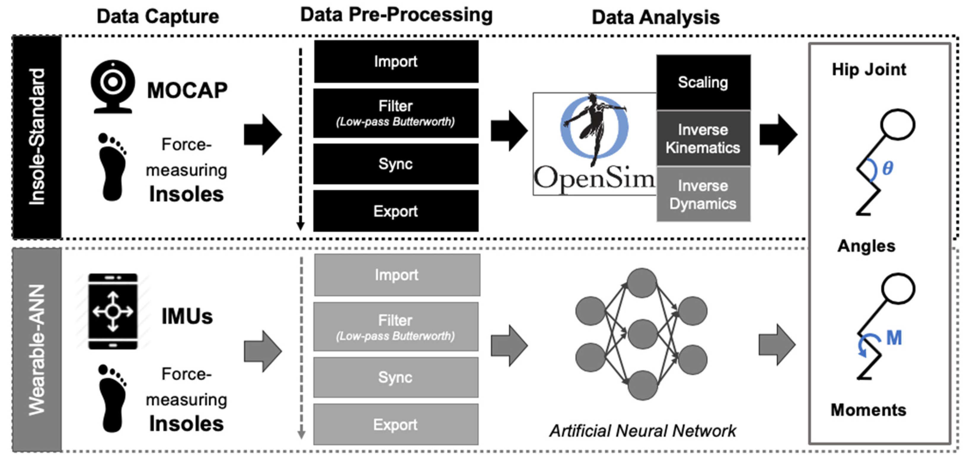
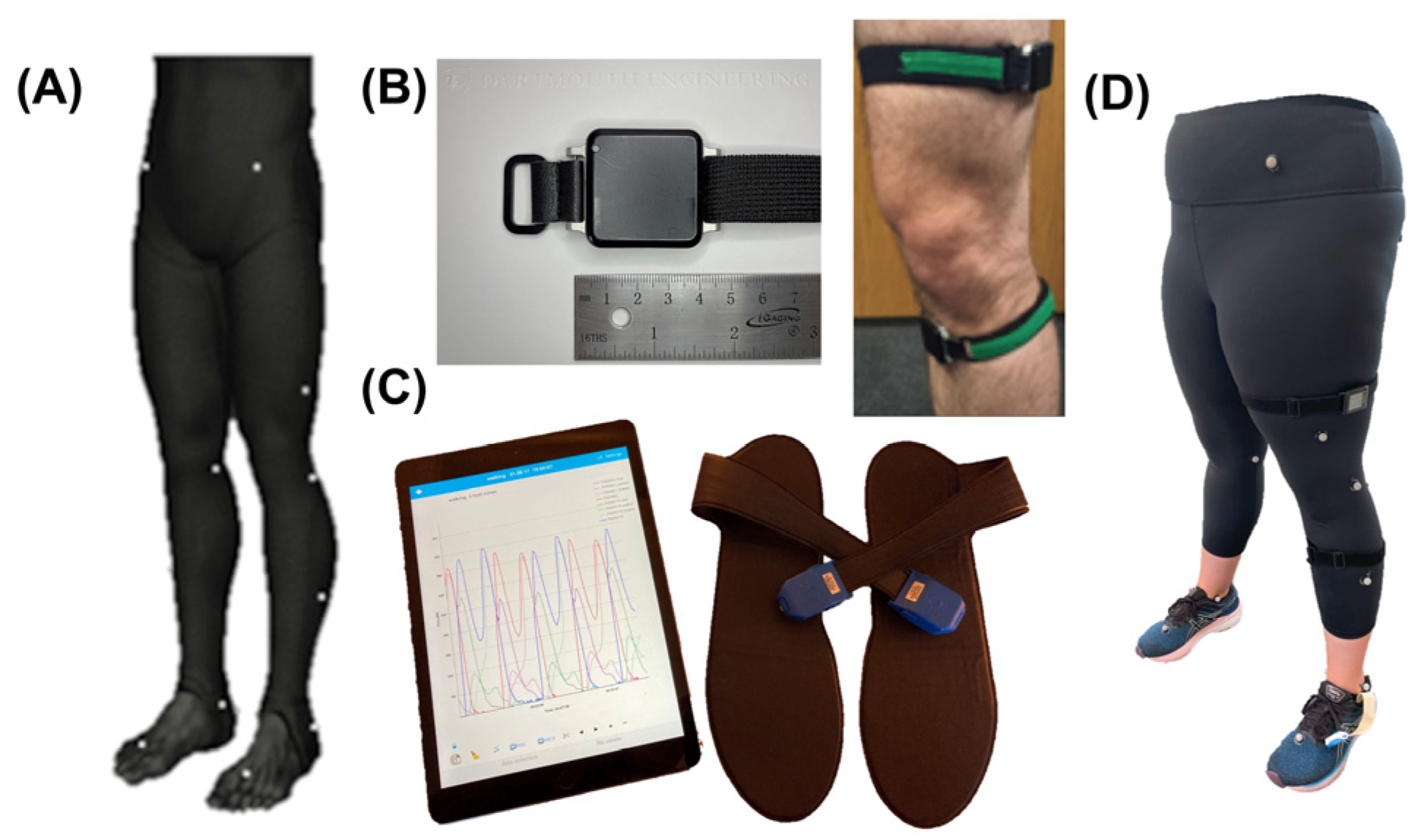
2.1. Data Capture
2.2. Data Pre-Processing
2.2.1. Overview
2.2.2. MATLAB Pre-Processing
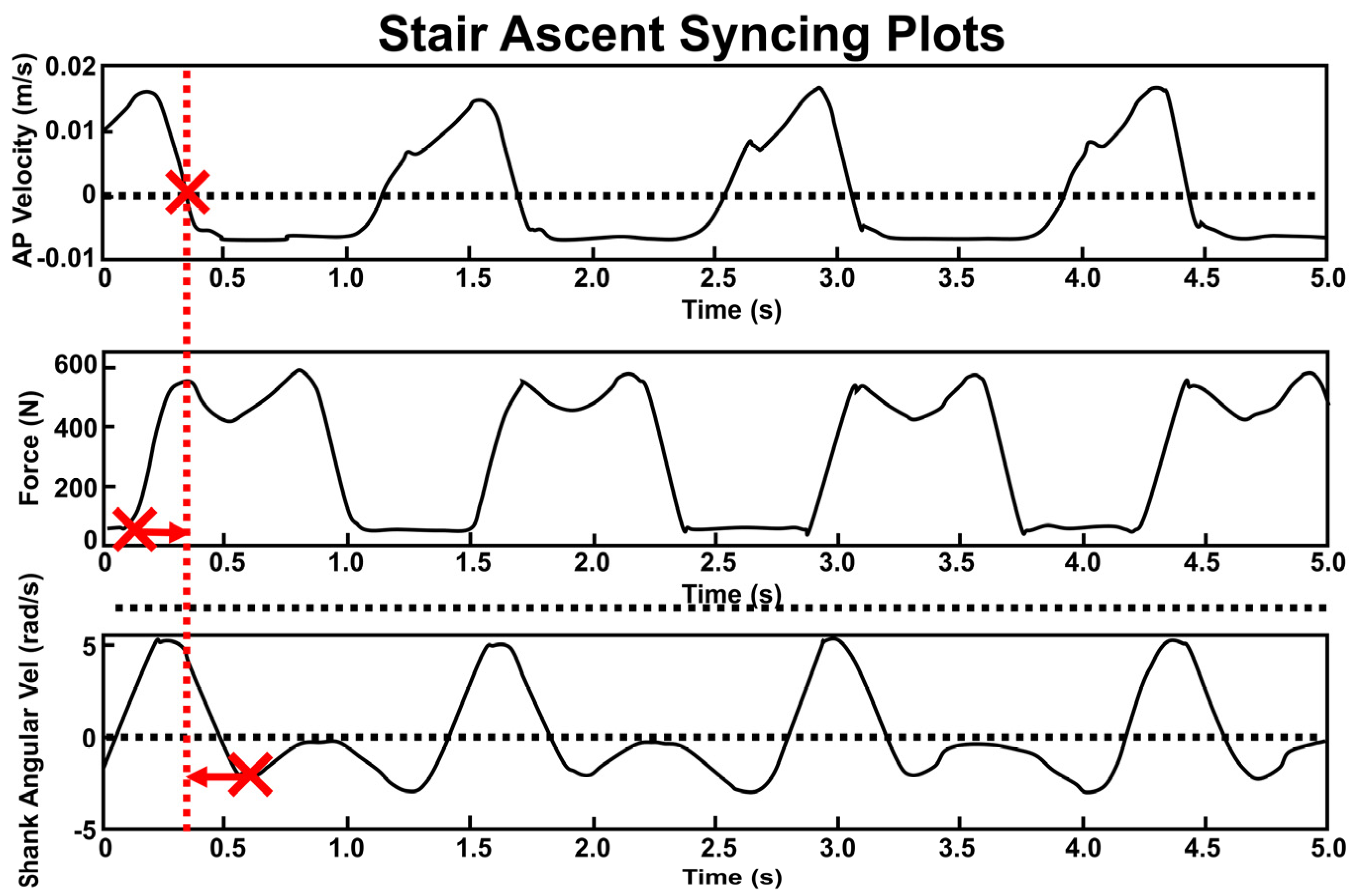
2.2.3. Temporal Synchronization (Figure 3)
2.2.4. OpenSim Workflow
2.2.5. ANN Workflow
3. Results
3.1. Stair Ascent on the Exercise Machine
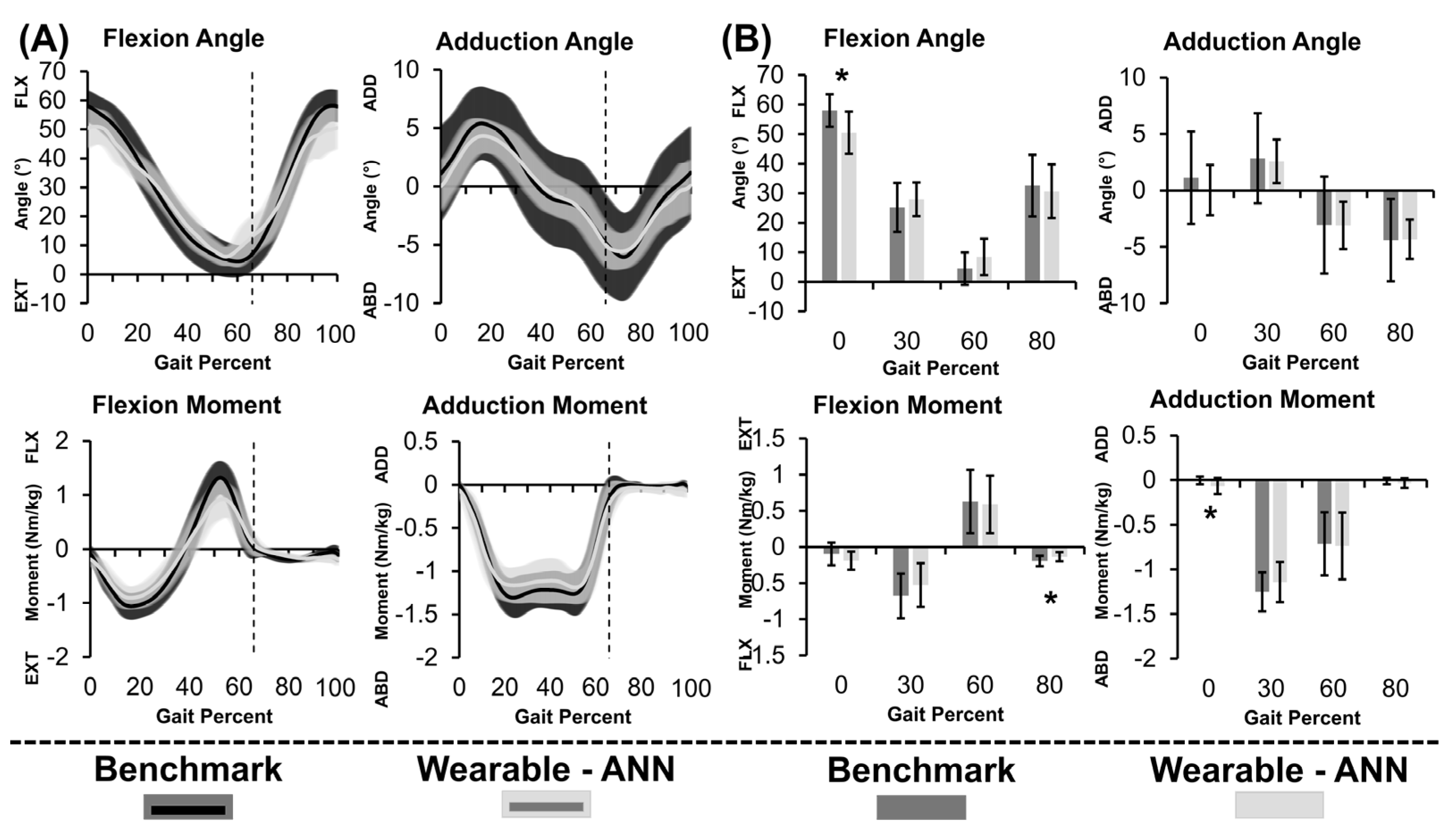
3.2. Gold-Standard Approach
3.3. Wearable-ANN Approach
4. Discussion
4.1. Overview
4.2. Stair Ascent on Exercise Machine
4.3. Gold-Standard Approach
4.4. Wearable-ANN Approach
4.5. Limitations
5. Conclusions
Author Contributions
Funding
Institutional Review Board Statement
Informed Consent Statement
Data Availability Statement
Acknowledgments
Conflicts of Interest
References
- Felson, D.T. Osteoarthritis as a Disease of Mechanics. Osteoarthr. Cartil. 2013, 21, 10–15. [Google Scholar] [CrossRef] [PubMed]
- Heller, M.O.; Bergmann, G.; Deuretzbacher, G.; Dürselen, L.; Pohl, M.; Claes, L.; Haas, N.P.; Duda, G.N. Musculo-Skeletal Loading Conditions at the Hip during Walking and Stair Climbing. J. Biomech. 2001, 34, 883–893. [Google Scholar] [CrossRef] [PubMed]
- Kassi, J.-P.; Heller, M.O.; Stoeckle, U.; Perka, C.; Duda, G.N. Stair Climbing Is More Critical than Walking in Pre-Clinical Assessment of Primary Stability in Cementless THA in Vitro. J. Biomech. 2005, 38, 1143–1154. [Google Scholar] [CrossRef] [PubMed]
- Kirkwood, R.N.; Culham, E.G.; Costigan, P. Hip Moments During Level Walking, Stair Climbing, and Exercise in Individuals Aged 55 Years or Older. Phys. Ther. 1999, 79, 360–370. [Google Scholar] [CrossRef] [PubMed]
- Röling, M.; Mathijssen, N.; Bloem, R. Incidence of Symptomatic Femoroacetabular Impingement in the General Population: A Prospective Registration Study. J. Hip Preserv. Surg. 2016, 3, 203–207. [Google Scholar] [CrossRef]
- Steiner, C.; Andrews, R.; Barrett, M.; Weiss, A. HCUP Projections: Mobility/Orthopaedic Procedures 2003 to 2012. 2012. Available online: http://www.hcup-us.ahrq.gov/reports/projections/2012-03.pdf (accessed on 3 March 2022).
- Swanson, E.; Schmalzried, T.; Dorey, F. Activity Recommendations After Total Hip and Knee Arthroplasty. J. Arthroplast. 2009, 24, 120–126. [Google Scholar] [CrossRef]
- Bevill, S.; Bevill, G.; Penmetsa, J.; Petrella, A.; Rullkoetter, P. Finite Element Simulation of Early Creep and Wear in Total Hip Arthroplasty. J. Biomech. 2005, 38, 2365–2374. [Google Scholar] [CrossRef]
- Callaghan, J.; Pedersen, D.; Johnston, R.; Brown, T. Clinical Biomechanics of Wear in Total Hip Arthroplasty. Iowa Orthop. J. 2003, 23, 1–12. [Google Scholar]
- Hamacher, D.; Bertram, D.; Fölsch, C.; Schega, L. Evaluation of a Visual Feedback System in Gait Retraining: A Pilot Study. Gait Posture 2012, 36, 182–186. [Google Scholar] [CrossRef]
- Haynes, R.; Pöll, R.; Miles, A.; Weston, R. Failure of Femoral Head Fixation: A Cadaveric Analysis of Lag Screw Cut-out with the Gamma Locking Nail and AO Dynamic Hip Screw. Injury 1997, 28, 337–341. [Google Scholar] [CrossRef]
- Luo, C.; Wu, X.; Wan, Y.; Liao, J.; Cheng, Q.; Tian, M.; Bai, Z.; Huang, W. Femoral Stress Changes after Total Hip Arthroplasty with the Ribbed Prosthesis: A Finite Element Analysis. BioMed Res. Int. 2020, 2020, 6783936. [Google Scholar] [CrossRef] [PubMed]
- Munro, J.; Millar, J.; Fernandez, J.; Walker, C.G.; Howie, D.; Shim, V. Risk Analysis of Patients with an Osteolytic Acetabular Defect after Total Hip Arthroplasty Using Subject-Specific Finite-Element Modelling. Bone Jt. J. 2018, 100-B, 1455–1462. [Google Scholar] [CrossRef] [PubMed]
- Nunn, D.; Freeman, M.; Tanner, K.; Bonfield, W. Torsional Stability of the Femoral Component of Hip Arthroplasty. Response to an Anteriorly Applied Load. J. Bone Jt. Surg. Br. Vol. 1989, 71-B, 452–455. [Google Scholar] [CrossRef] [PubMed]
- Szivek, J.; Benjamin, J.; Anderson, P. An Experimental Method for the Application of Lateral Muscle Loading and Its Effect on Femoral Strain Distributions. Med. Eng. Phys. 2000, 22, 109–116. [Google Scholar] [CrossRef]
- Watanabe, Y.; Shiba, N.; Matsuo, S.; Higuchi, F.; Tagawa, Y.; Inoue, A. Biomechanical Study of the Resurfacing Hip Arthroplasty. J. Arthroplast. 2000, 15, 505–511. [Google Scholar] [CrossRef]
- Delp, S.; Anderson, F.; Arnold, A.; Loan, P.; Habib, A.; John, C.; Guendelman, E.; Thelen, D. OpenSim: Open-Source Software to Create and Analyze Dynamic Simulations of Movement. IEEE Trans. Biomed. Eng. 2007, 54, 1940–1950. [Google Scholar] [CrossRef]
- Seth, A.; Hicks, J.; Uchida, T.; Habib, A.; Dembia, C.L.; Dunne, J.; Ong, C.; DeMers, M.; Rajagopal, A.; Millard, M.; et al. OpenSim: Simulating Musculoskeletal Dynamics and Neuromuscular Control to Study Human and Animal Movement. PLoS Comput. Biol. 2018, 14, e1006223. [Google Scholar] [CrossRef]
- Silva, M.; Moreira, P.; Rocha, H. Development of a Low Cost Force Platform for Biomechanical Parameters Analysis. Res. Biomed. Eng. 2017, 33, 259–268. [Google Scholar] [CrossRef]
- Steiling, S.; Morgan, J. Optitrack Software Comparison Tool. Available online: https://optitrack.com/software/compare/ (accessed on 3 March 2022).
- Steiling, S.; Morgan, J. OptiTrack’s S250e Ethernet Motion Capture Camera Now Available to Customers Worldwide. Available online: https://optitrack.com/about/press/20101116.html#:~:text=The%20S250e%20motion%20capture%20camera,%2C%20or%20visit%20optitrack.com (accessed on 2 March 2022).
- Peebles, A.; Maguire, L.; Renner, K.; Queen, R. Validity and Repeatability of Single-Sensor Loadsol Insoles during Landing. Sensors 2018, 18, 4082. [Google Scholar] [CrossRef]
- Renner, K.; Williams, D.; Queen, R. The Reliability and Validity of the Loadsol® under Various Walking and Running Conditions. Sensors 2019, 19, 265. [Google Scholar] [CrossRef]
- Robert-Lachaine, X.; Mecheri, H.; Larue, C.; Plamondon, A. Validation of Inertial Measurement Units with an Optoelectronic System for Whole-Body Motion Analysis. Med. Biol. Eng. Comput. 2017, 55, 609–619. [Google Scholar] [CrossRef] [PubMed]
- Dorschky, E.; Nitschke, M.; Seifer, A.; van den Bogert, A.; Eskofier, B. Estimation of Gait Kinematics and Kinetics from Inertial Sensor Data Using Optimal Control of Musculoskeletal Models. J. Biomech. 2019, 95, 109278. [Google Scholar] [CrossRef] [PubMed]
- Konrath, J.; Karatsidis, A.; Schepers, H.; Bellusci, G.; de Zee, M.; Andersen, M. Estimation of the Knee Adduction Moment and Joint Contact Force during Daily Living Activities Using Inertial Motion Capture. Sensors 2019, 19, 1681. [Google Scholar] [CrossRef] [PubMed]
- van den Noort, J.; van der Esch, M.; Steultjens, M.; Dekker, J.; Schepers, M.; Veltink, P.; Harlaar, J. Ambulatory Measurement of the Knee Adduction Moment in Patients with Osteoarthritis of the Knee. J. Biomech. 2013, 46, 43–49. [Google Scholar] [CrossRef]
- McCabe, M.V.; Van Citters, D.W.; Chapman, R.M. Developing a Method for Quantifying Hip Joint Angles and Moments during Walking Using Neural Networks and Wearables. Comput. Methods Biomech. Biomed. Eng. 2022, 26, 1–11. [Google Scholar] [CrossRef]
- Gurchiek, R.; Cheney, N.; McGinnis, R. Estimating Biomechanical Time-Series with Wearable Sensors: A Systematic Review of Machine Learning Techniques. Sensors 2019, 19, 5227. [Google Scholar] [CrossRef]
- Lim, H.; Kim, B.; Park, S. Prediction of Lower Limb Kinetics and Kinematics during Walking by a Single IMU on the Lower Back Using Machine Learning. Sensors 2019, 20, 130. [Google Scholar] [CrossRef]
- Mundt, M.; Koeppe, A.; David, S.; Witter, T.; Bamer, F.; Potthast, W.; Markert, B. Estimation of Gait Mechanics Based on Simulated and Measured IMU Data Using an Artificial Neural Network. Front. Bioeng. Biotechnol. 2020, 8, 41. [Google Scholar] [CrossRef]
- Stetter, B.; Krafft, F.; Ringhof, S.; Stein, T.; Sell, S. A Machine Learning and Wearable Sensor Based Approach to Estimate External Knee Flexion and Adduction Moments During Various Locomotion Tasks. Front. Bioeng. Biotechnol. 2020, 8, 9. [Google Scholar] [CrossRef]
- Svenningsen, S.; Terjesen, T.; Auflem, M.; Berg, V. Hip Motion Related to Age and Sex. Acta Orthop. Scand. 1989, 60, 97–100. [Google Scholar] [CrossRef]
- Collins, T.; Ghoussayni, S.; Ewins, D.; Kent, J. A Six Degrees-of-Freedom Marker Set for Gait Analysis: Repeatability and Comparison with a Modified Helen Hayes Set. Gait Posture 2009, 30, 173–180. [Google Scholar] [CrossRef] [PubMed]
- Kadaba, M.; Ramakrishnan, H.; Wootten, M. Measurement of Lower Extremity Kinematics during Level Walking. J. Orthop. Res. 1990, 8, 383–392. [Google Scholar] [CrossRef] [PubMed]
- Elias, L.; Bryden, M.; Bulman-Fleming, M. Footedness Is a Better Predictor than Is Handedness of Emotional Lateralization. Neuropsychologia 1998, 36, 37–43. [Google Scholar] [CrossRef]
- Coley, B.; Najafi, B.; Paraschiv-Ionescu, A.; Aminian, K. Stair Climbing Detection during Daily Physical Activity Using a Miniature Gyroscope. Gait Posture 2005, 22, 287–294. [Google Scholar] [CrossRef]
- Yang, S.; Zhang, J.; Novak, A.; Brouwer, B.; Li, Q. Estimation of Spatio-Temporal Parameters for Post-Stroke Hemiparetic Gait Using Inertial Sensors. Gait Posture 2013, 37, 354–358. [Google Scholar] [CrossRef]
- Foster, R.; De Asha, A.; Reeves, N.; Maganaris, C.; Buckley, J. Stair-Specific Algorithms for Identification of Touch-down and Foot-off When Descending or Ascending a Non-Instrumented Staircase. Gait Posture 2014, 39, 816–821. [Google Scholar] [CrossRef]
- O’Connor, C.; Thorpe, S.; O’Malley, M.; Vaughan, C. Automatic Detection of Gait Events Using Kinematic Data. Gait Posture 2007, 25, 469–474. [Google Scholar] [CrossRef]
- Zeni, J.; Richards, J.; Higginson, J. Two Simple Methods for Determining Gait Events during Treadmill and Overground Walking Using Kinematic Data. Gait Posture 2008, 27, 710–714. [Google Scholar] [CrossRef] [PubMed]
- Bergmann, J.; Mayagoitia, R.; Smith, I. A Novel Method for Determining Ground-Referenced Contacts during Stair Ascent: Comparing Relative Hip Position to Quiet Standing Hip Height. Gait Posture 2010, 31, 164–168. [Google Scholar] [CrossRef]
- Higginson, J.; John, C. Tutorial 3—Scaling, Inverse Kinematics, and Inverse Dynamics. Available online: https://simtk-confluence.stanford.edu:8443/display/OpenSim/Tutorial+3+-+Scaling%2C+Inverse+Kinematics%2C+and+Inverse+Dynamics#Tutorial3-Scaling,InverseKinematics,andInverseDynamics-III.ScalingAMusculoskeletalModel (accessed on 17 May 2020).
- Thelen, D.; Ajay, S.; Anderson, F.; Delp, S. Gait 2392 and 2354 Models. Available online: https://simtk-confluence.stanford.edu/display/OpenSim/Gait%2B2392%2Band%2B2354%2BModels (accessed on 8 March 2020).
- The National Center for Simulation in Rehabilitation Research How Scaling Works. Available online: https://simtk-confluence.stanford.edu/display/OpenSim/How+Scaling+Works (accessed on 31 July 2020).
- The National Center for Simulation in Rehabilitation Research How Inverse Kinematics Works. Available online: https://simtk-confluence.stanford.edu/display/OpenSim/How+Inverse+Kinematics+Works (accessed on 31 July 2020).
- Dudum, K.; Deschamps, J.; Gutierrez-Franco, J.; Kraemer, L.; Gonzalez-Smith, A.; Dandekar, E.; Hazelwood, S.; Klisch, S. Using OpenSim to Predict Knee Joint Moments during Cycling. In Proceedings of the 2015 Summer Biomechanics, Bioengineering, and Biotransport Conference Proceedings, Snowbird, UT, USA, 17 June 2015. [Google Scholar]
- Baughman, D.; Liu, Y. Neural Networks in Bioprocessing and Chemical Engineering; Academic Press: Cambridge, MA, USA, 1996. [Google Scholar]
- Wouda, F.; Giuberti, M.; Bellusci, G.; Maartens, E.; Reenalda, J.; van Beijnum, B.; Veltink, P. Estimation of Vertical Ground Reaction Forces and Sagittal Knee Kinematics During Running Using Three Inertial Sensors. Front. Physiol. 2018, 9, 218. [Google Scholar] [CrossRef]
- Costigan, P.; Deluzio, K.; Wyss, U. Knee and Hip Kinetics during Normal Stair Climbing. Gait Posture 2002, 16, 31–37. [Google Scholar] [CrossRef] [PubMed]
- Eng, J.; Winter, D. Kinetic Analysis of the Lower Limbs during Walking: What Information Can Be Gained from a Three-Dimensional Model? J. Biomech. 1995, 28, 753–758. [Google Scholar] [CrossRef] [PubMed]
- Protopapadaki, A.; Drechsler, W.; Cramp, M.; Coutts, F.; Scott, O. Hip, Knee, Ankle Kinematics and Kinetics during Stair Ascent and Descent in Healthy Young Individuals. Clin. Biomech. 2007, 22, 203–210. [Google Scholar] [CrossRef] [PubMed]
- Riener, R.; Rabuffetti, M.; Frigo, C. Stair Ascent and Descent at Different Inclinations. Gait Posture 2002, 15, 32–44. [Google Scholar] [CrossRef] [PubMed]
- Lin, H.; Lu, T.; Hsu, H. Three-Dimensional Analysis of Kinematic and Kinetic Coordination of the Lower Limb Joints during Stair Ascent and Descent. Biomed. Eng. Appl. Basis Commun. 2004, 16, 101–108. [Google Scholar] [CrossRef]
- Pizzolato, C.; Reggiani, M.; Modenese, L.; Lloyd, D. Real-Time Inverse Kinematics and Inverse Dynamics for Lower Limb Applications Using OpenSim. Comput. Methods Biomech. Biomed. Eng. 2017, 20, 436–445. [Google Scholar] [CrossRef]
- Kim, H.; Sakurai, S.; Ahn, J. Errors in the Measurement of Center of Pressure (CoP) Computed with Force Plate Affect on 3D Lower Limb Joint Moment During Gait. Int. J. Sport Health Sci. 2007, 5, 71–82. [Google Scholar] [CrossRef]
- McCaw, S.; DeVita, P. Errors in Alignment of Center of Pressure and Foot Coordinates Affect Predicted Lower Extremity Torques. J. Biomech. 1995, 28, 985–988. [Google Scholar] [CrossRef]
- Chiu, M.; Wu, H.; Chang, L. Gait Speed and Gender Effects on Center of Pressure Progression during Normal Walking. Gait Posture 2013, 37, 43–48. [Google Scholar] [CrossRef]
- Forner Cordero, A.; Koopman, H.; van der Helm, F. Inverse Dynamics Calculations during Gait with Restricted Ground Reaction Force Information from Pressure Insoles. Gait Posture 2006, 23, 189–199. [Google Scholar] [CrossRef]
- Forner Cordero, A.; Koopman, H.; van der Helm, F. Use of Pressure Insoles to Calculate the Complete Ground Reaction Forces. J. Biomech. 2004, 37, 1427–1432. [Google Scholar] [CrossRef] [PubMed]
- Hullfish, T.; Baxter, J. A Simple Instrumented Insole Algorithm to Estimate Plantar Flexion Moments. Gait Posture 2020, 79, 92–95. [Google Scholar] [CrossRef] [PubMed]
- Jönsson, M.; Munkhammar, T.; Norrbrand, L.; Berg, H. Foot Centre of Pressure and Ground Reaction Force during Quadriceps Resistance Exercises; a Comparison between Force Plates and a Pressure Insole System. J. Biomech. 2019, 87, 206–210. [Google Scholar] [CrossRef] [PubMed]
- Jung, Y.; Jung, M.; Lee, K.; Koo, S. Ground Reaction Force Estimation Using an Insole-Type Pressure Mat and Joint Kinematics during Walking. J. Biomech. 2014, 47, 2693–2699. [Google Scholar] [CrossRef] [PubMed]
- Bowden, M.; Balasubramanian, C.; Neptune, R.; Kautz, S. Anterior-Posterior Ground Reaction Forces as a Measure of Paretic Leg Contribution in Hemiparetic Walking. Stroke 2006, 37, 872–876. [Google Scholar] [CrossRef]
- White, R.; Agouris, I.; Selbie, R.D.; Kirkpatrick, M. The Variability of Force Platform Data in Normal and Cerebral Palsy Gait. Clin. Biomech. 1999, 14, 185–192. [Google Scholar] [CrossRef]
- Saeb, S.; Lonini, L.; Jayaraman, A.; Mohr, D.; Kording, K. The Need to Approximate the Use-Case in Clinical Machine Learning. GigaScience 2017, 6, gix019. [Google Scholar] [CrossRef]


| Gait (%) | Method | S θ (°) | S µ (Nm/kg) | F θ (°) | F µ (Nm/kg) |
|---|---|---|---|---|---|
| 0 | B-Mk | 58.0 ± 5.5 | −0.1 ± 0.2 | 1.1 ± 4.1 | −0.003 ± 0.04 |
| W-ANN | 50.5 ± 7.2 | −0.2 ± 0.1 | 0.02 ± 2.2 | −0.07 ± 0.09 | |
| 30 | B-Mk | 25.2 ± 8.3 | −0.7 ± 0.3 | 2.8 ± 4.0 | −1.3 ± 0.2 |
| W-ANN | 27.9 ± 5.7 | −0.5 ± 0.3 | 2.6 ± 1.9 | −1.1 ± 0.2 | |
| 60 | B-Mk | 4.5 ± 5.5 | 0.6 ± 0.4 | −3.1 ± 4.3 | −0.7 ± 0.4 |
| W-ANN | 8.4 ± 6.2 | 0.6 ± 0.4 | −3.1 ± 2.1 | −0.7 ± 0.4 | |
| 80 | B-Mk | 32.6 ± 10.4 | −0.2 ± 0.1 | −4.4 ± 3.7 | −0.01 ± 0.04 |
| W-ANN | 30.7 ± 9.1 | −0.1 ± 0.1 | −4.3 ± 1.7 | −0.03 ± 0.05 | |
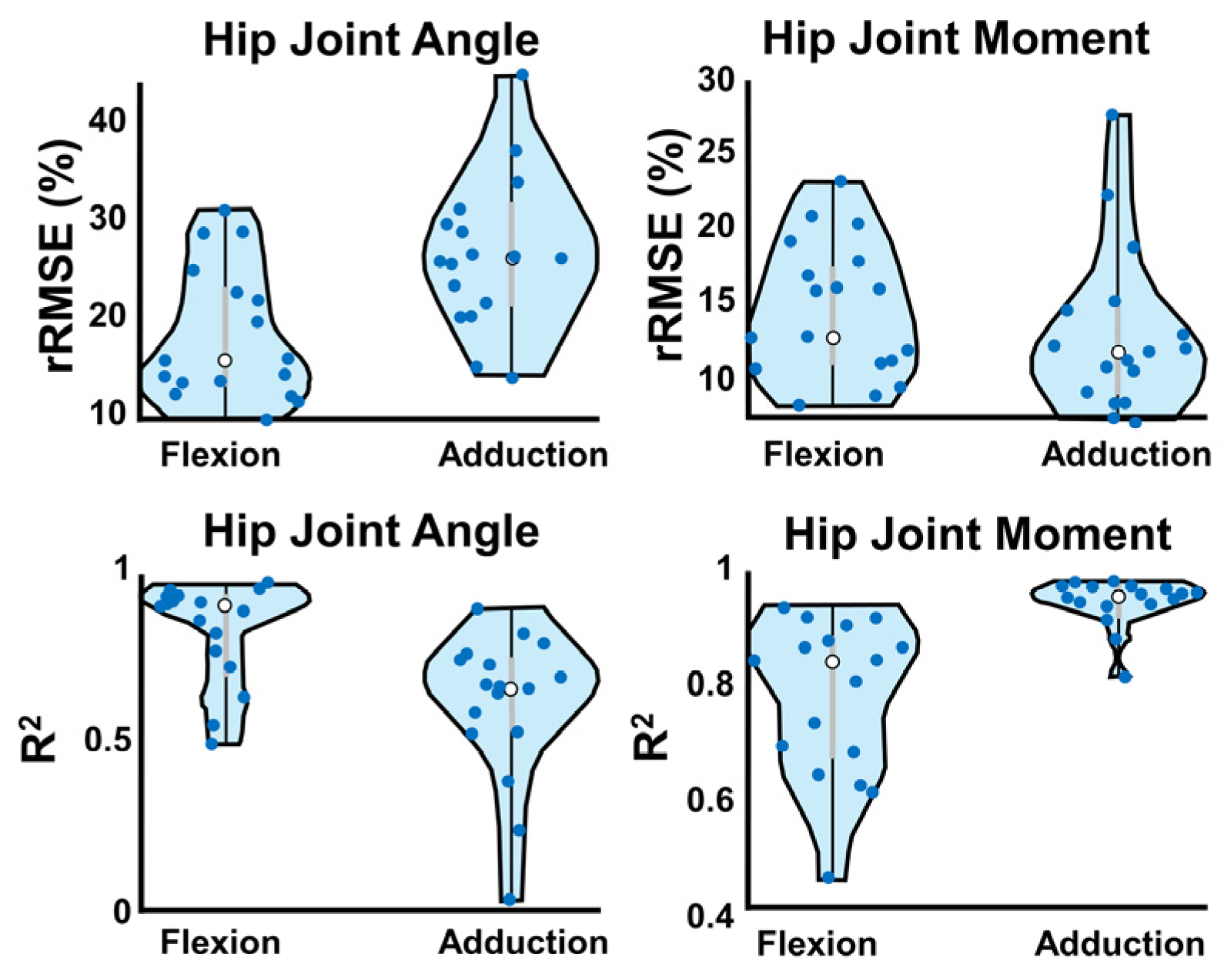
| R2 | 0.80 ± 0.02 | 0.59 ± 0.02 | 0.77 ± 0.02 | 0.93 ± 0.01 | |
| rRMSE | 17.7 ± 1.2 | 26.4 ± 1.4 | 14.1 ± 0.8 | 12.7 ± 1.1 | |
Disclaimer/Publisher’s Note: The statements, opinions and data contained in all publications are solely those of the individual author(s) and contributor(s) and not of MDPI and/or the editor(s). MDPI and/or the editor(s) disclaim responsibility for any injury to people or property resulting from any ideas, methods, instructions or products referred to in the content. |
© 2023 by the authors. Licensee MDPI, Basel, Switzerland. This article is an open access article distributed under the terms and conditions of the Creative Commons Attribution (CC BY) license (https://creativecommons.org/licenses/by/4.0/).
Share and Cite
McCabe, M.V.; Van Citters, D.W.; Chapman, R.M. Hip Joint Angles and Moments during Stair Ascent Using Neural Networks and Wearable Sensors. Bioengineering 2023, 10, 784. https://doi.org/10.3390/bioengineering10070784
McCabe MV, Van Citters DW, Chapman RM. Hip Joint Angles and Moments during Stair Ascent Using Neural Networks and Wearable Sensors. Bioengineering. 2023; 10(7):784. https://doi.org/10.3390/bioengineering10070784
Chicago/Turabian StyleMcCabe, Megan V., Douglas W. Van Citters, and Ryan M. Chapman. 2023. "Hip Joint Angles and Moments during Stair Ascent Using Neural Networks and Wearable Sensors" Bioengineering 10, no. 7: 784. https://doi.org/10.3390/bioengineering10070784
APA StyleMcCabe, M. V., Van Citters, D. W., & Chapman, R. M. (2023). Hip Joint Angles and Moments during Stair Ascent Using Neural Networks and Wearable Sensors. Bioengineering, 10(7), 784. https://doi.org/10.3390/bioengineering10070784