
High-Speed and Accurate Diagnosis of Gastrointestinal Disease: Learning on Endoscopy Images Using Lightweight Transformer with Local Feature Attention

Abstract
:1. Introduction
2. Materials and Methods
2.1. Data Collection and Preprocessing
2.2. Model Architecture
2.2.1. Vision Transformer
2.2.2. Proposed Model—FLATer
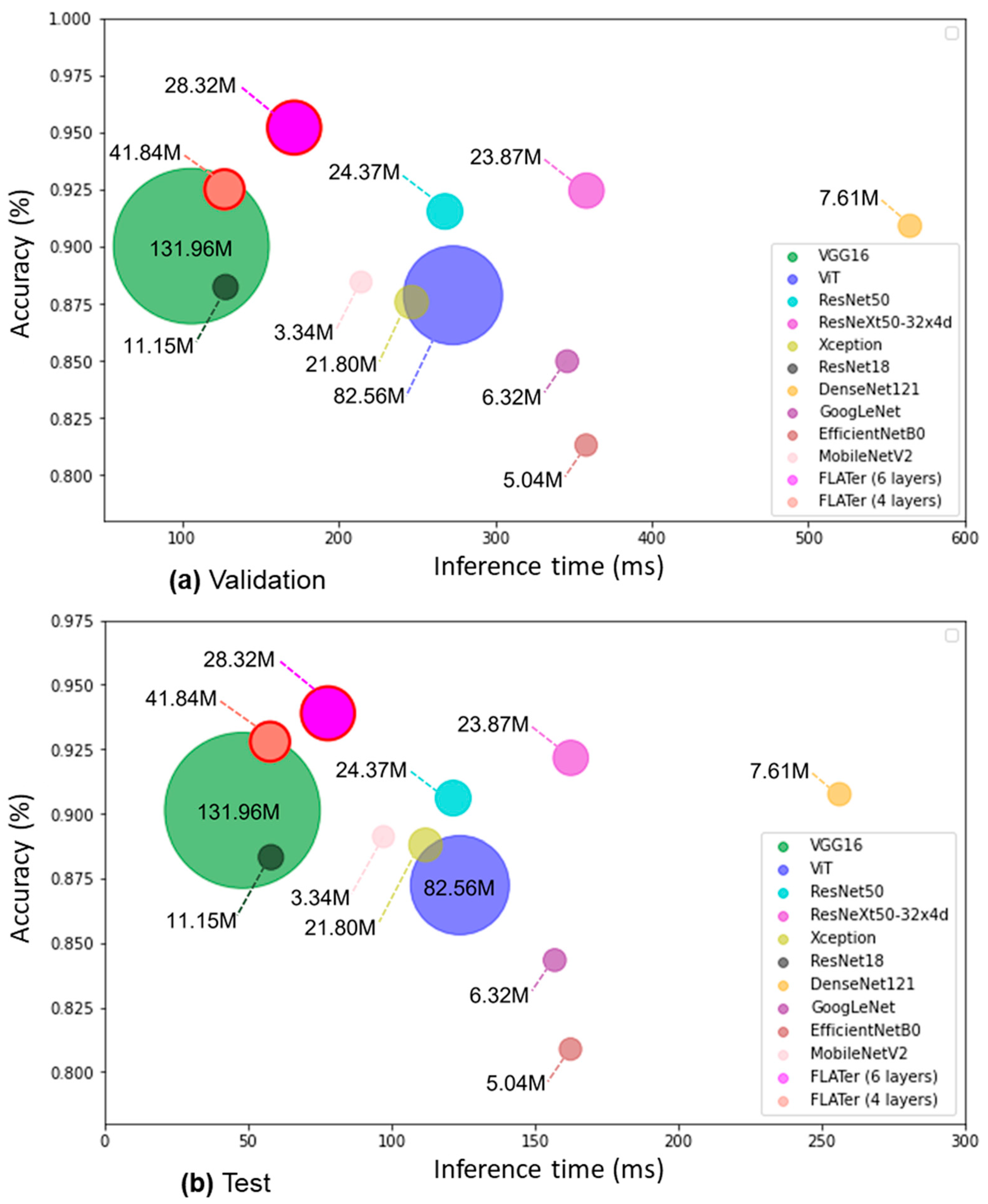
2.2.3. Comparison Models
2.3. Experimental Set Up
2.4. Model Evaluation
3. Results
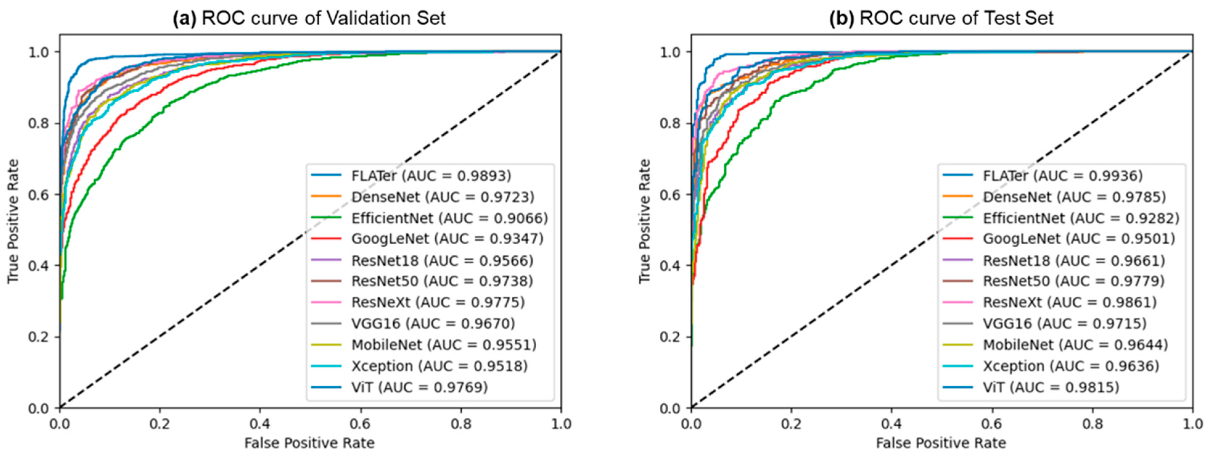
3.1. Binary Classification Results
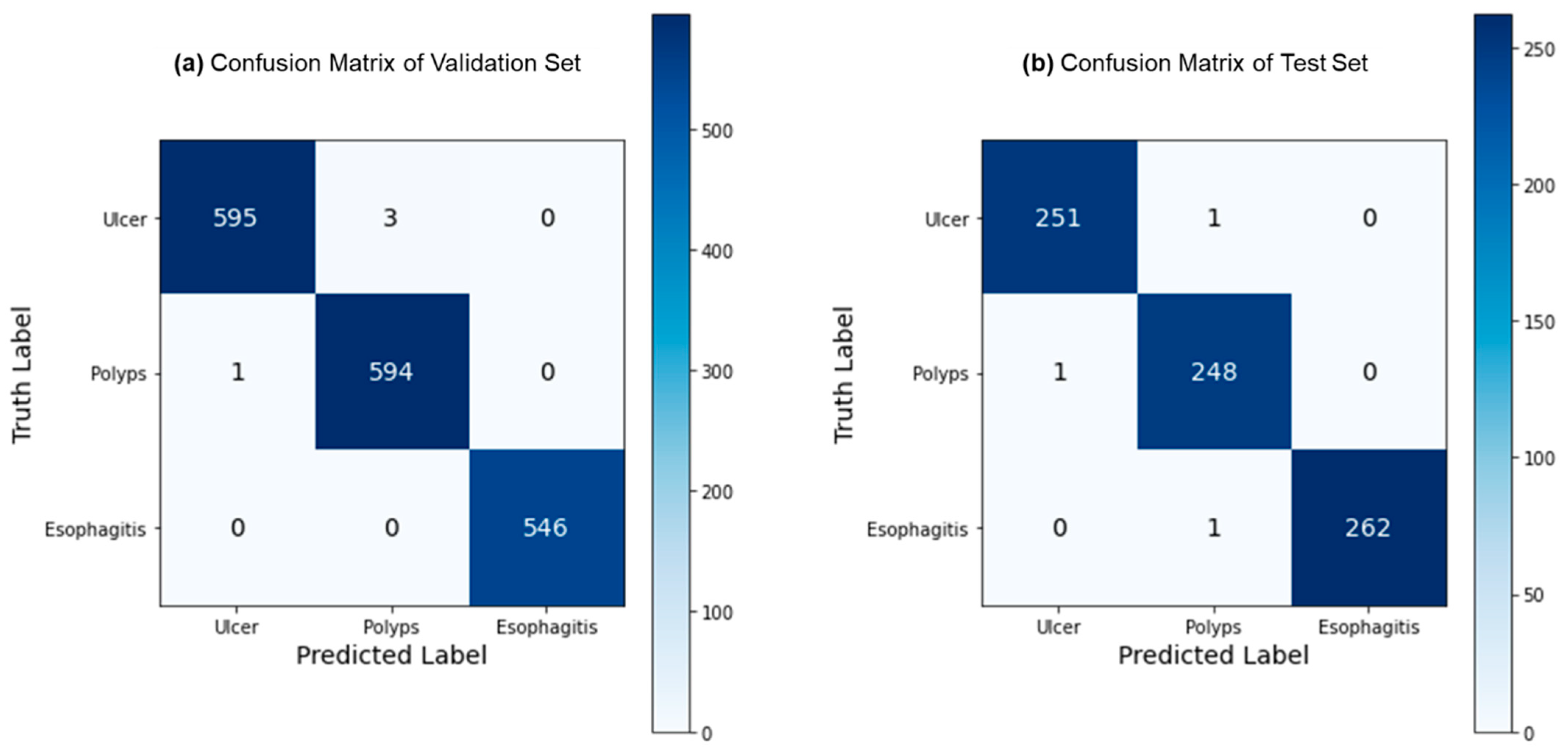
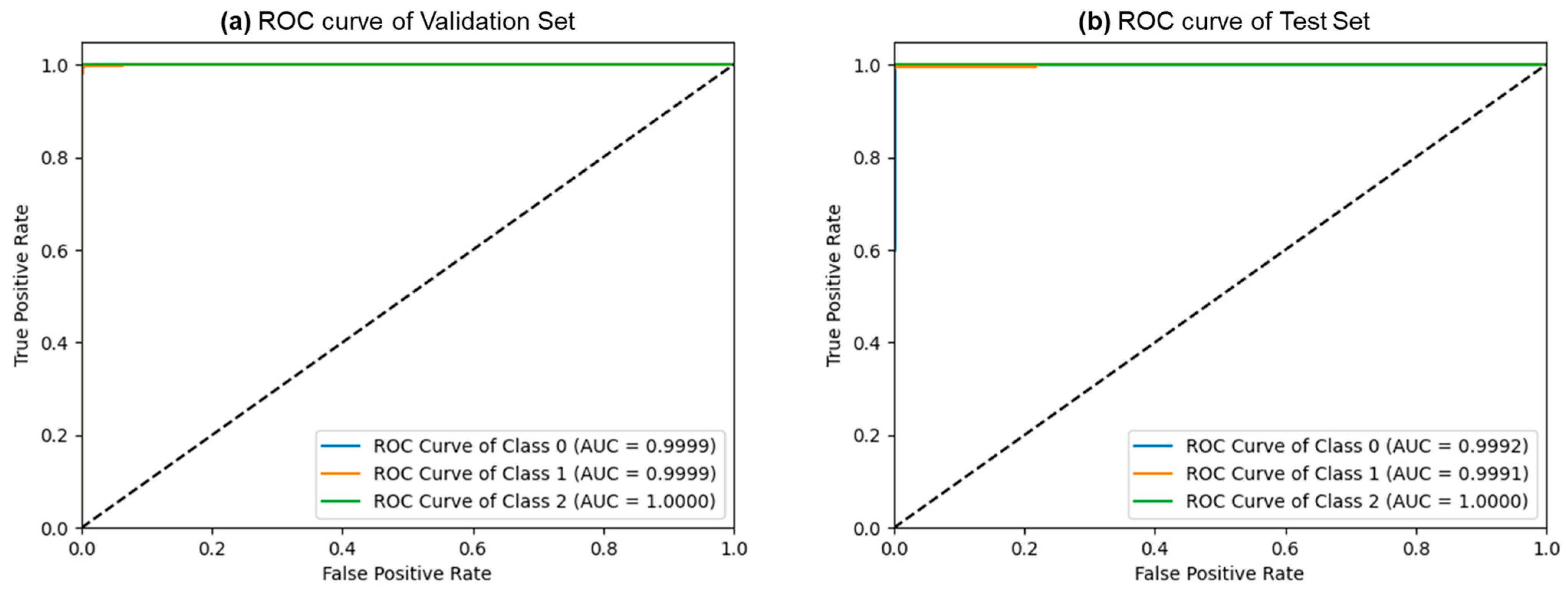
3.2. Ternary Classification Results
3.3. Ablation Study Results
4. Discussion
5. Conclusions
Author Contributions
Funding
Institutional Review Board Statement
Informed Consent Statement
Data Availability Statement
Conflicts of Interest
References
- Chen, W.; Zheng, R.; Baade, P.D.; Zhang, S.; Zeng, H.; Bray, F.; Jemal, A.; Yu, X.Q.; He, J. Cancer statistics in China, 2015. Cancer J. Clin. 2016, 66, 115–132. [Google Scholar] [CrossRef]
- Bray, F.; Ferlay, J.; Soerjomataram, I.; Siegel, R.L.; Torre, L.A.; Jemal, A. Global cancer statistics 2018: GLOBOCAN estimates of incidence and mortality worldwide for 36 cancers in 185 countries. Cancer J. Clin. 2018, 68, 394–424. [Google Scholar] [CrossRef]
- Lee, J.M.; Park, Y.M.; Yun, J.S.; Ahn, Y.B.; Lee, K.M.; Kim, D.B.; Lee, J.M.; Han, K.; Ko, S.H. The association between nonalcoholic fatty liver disease and esophageal, stomach, or colorectal cancer: National population-based cohort study. PLoS ONE 2020, 15, e0226351. [Google Scholar] [CrossRef]
- Leufkens, A.M.; van Oijen, M.G.H.; Vleggaar, F.P.; Siersema, P.D. Factors influencing the miss rate of polyps in a back-to-back colonoscopy study. Endoscopy 2012, 44, 470–475. [Google Scholar] [CrossRef] [PubMed]
- Rogler, G. Chronic ulcerative colitis and colorectal cancer. Cancer Lett. 2014, 345, 235–241. [Google Scholar] [CrossRef] [PubMed]
- Khan, M.A.; Khan, M.A.; Ahmed, F.; Mittal, M.; Goyal, L.M.; Hemanth, D.J.; Satapathy, S.C. Gastrointestinal diseases segmentation and classification based on duo-deep architectures. Pattern Recognit. Lett. 2020, 131, 193–204. [Google Scholar] [CrossRef]
- Gomez Torrijos, E.; Gonzalez-Mendiola, R.; Alvarado, M.; Avila, R.; Prieto-Garcia, A.; Valbuena, T.; Borja, J.; Infante, S.; Lopez, M.P.; Marchan, E. Eosinophilic esophagitis: Review and update. Front. Med. 2018, 5, 247. [Google Scholar] [CrossRef] [PubMed]
- Sumiyama, K. Past and current trends in endoscopic diagnosis for early stage gastric cancer in Japan. Gastric Cancer Off. J. Int. Gastric Cancer Assoc. Jpn. Gastric Cancer Assoc. 2017, 20 (Suppl. S1), 20–27. [Google Scholar] [CrossRef]
- Rahim, T.; Usman, M.A.; Shin, S.Y. A survey on contemporary computer-aided tumor, polyp, and ulcer detection methods in wireless capsule endoscopy imaging. Comput. Med. Imaging Graph. Off. J. Comput. Med. Imaging Soc. 2020, 85, 101767. [Google Scholar] [CrossRef] [PubMed]
- ASGE Technology Committee; Wang, A.; Banerjee, S.; Barth, B.A.; Bhat, Y.M.; Chauhan, S.; Gottlieb, K.T.; Konda, V.; Maple, J.T.; Murad, F.; et al. Wireless capsule endoscopy. Gastrointest. Endosc. 2013, 78, 805–815. [Google Scholar] [CrossRef]
- Dey, N.; Ashour, A.S.; Shi, F.; Sherratt, R.S. Wireless Capsule Gastrointestinal Endoscopy: Direction-of-Arrival Estimation Based Localization Survey. IEEE Rev. Biomed. Eng. 2017, 10, 2–11. [Google Scholar] [CrossRef]
- Iddan, G.; Meron, G.; Glukhovsky, A.; Swain, P. Wireless capsule endoscopy. Nature 2000, 405, 417. [Google Scholar] [CrossRef] [PubMed]
- Liaqat, A.; Khan, M.A.; Shah, J.H.; Sharif, M.; Yasmin, M.; Fernandes, S.L. Automated ulcer and bleeding classification from WCE images using multiple features fusion and selection. J. Mech. Med. Biol. 2018, 18, 1850038. [Google Scholar] [CrossRef]
- Hong, T.C.; Liou, J.M.; Yeh, C.C.; Yen, H.H.; Wu, M.S.; Lai, I.R.; Chen, C.C. Endoscopic submucosal dissection comparing with surgical resection in patients with early gastric cancer—A single center experience in Taiwan. J. Formos. Med. Assoc. 2020, 119, 1750–1757. [Google Scholar] [CrossRef]
- Ishihara, R.; Takeuchi, Y.; Chatani, R.; Kidu, T.; Inoue, T.; Hanaoka, N.; Yamamoto, S.; Higashino, K.; Uedo, N.; Iishi, H.; et al. Original article: Prospective evaluation of narrow-band imaging endoscopy for screening of esophageal squamous mucosal high-grade neoplasia in experienced and less experienced endoscopists. Dis. Esophagus Off. J. Int. Soc. Dis. Esophagus 2010, 23, 480–486. [Google Scholar] [CrossRef] [PubMed]
- Sindhu, C.P.; Valsan, V. Automatic detection of colonic polyps and tumor in wireless capsule endoscopy images using hybrid patch extraction and supervised classification. In Proceedings of the 2017 International Conference on Innovations in Information, Embedded and Communication Systems (ICIIECS), Coimbatore, India, 17–18 March 2017; pp. 1–5. [Google Scholar]
- Yeh, J.-Y.; Wu, T.-H.; Tsai, W.-J. Bleeding and Ulcer Detection Using Wireless Capsule Endoscopy Images. J. Softw. Eng. Appl. 2014, 7, 422–432. [Google Scholar] [CrossRef]
- Liu, Y.; Lin, D.; Li, L.; Chen, Y.; Wen, J.; Lin, Y.; He, X. Using machine-learning algorithms to identify patients at high risk of upper gastrointestinal lesions for endoscopy. J. Gastroenterol. Hepatol. 2021, 36, 2735–2744. [Google Scholar] [CrossRef]
- Khan, S.H.; Shah, N.S.; Nuzhat, R.; Majid, A.; Alquhayz, H.; Khan, A. Malaria parasite classification framework using a novel channel squeezed and boosted CNN. Microscopy 2022, 71, 271–282. [Google Scholar] [CrossRef]
- Majid, A.; Khan, M.A.; Yasmin, M.; Rehman, A.; Yousafzai, A.; Tariq, U. Classification of stomach infections: A paradigm of convolutional neural network along with classical features fusion and selection. Microsc. Res. Tech. 2020, 83, 562–576. [Google Scholar] [CrossRef]
- Komeda, Y.; Handa, H.; Matsui, R.; Hatori, S.; Yamamoto, R.; Sakurai, T.; Takenaka, M.; Hagiwara, S.; Nishida, N.; Kashida, H.; et al. Artificial intelligence-based endoscopic diagnosis of colorectal polyps using residual networks. PLoS ONE 2021, 16, e0253585. [Google Scholar] [CrossRef]
- Du, W.; Rao, N.; Dong, C.; Wang, Y.; Hu, D.; Zhu, L.; Zeng, B.; Gan, T. Automatic classification of esophageal disease in gastroscopic images using an efficient channel attention deep dense convolutional neural network. Biomed. Opt. Express 2021, 12, 3066–3081. [Google Scholar] [CrossRef] [PubMed]
- Yogapriya, J.; Chandran, V.; Sumithra, M.G.; Anitha, P.; Jenopaul, P.; Dhas, C.S.G. Gastrointestinal Tract Disease Classification from Wireless Endoscopy Images Using Pretrained Deep Learning Model. Comput. Math. Methods Med. 2021, 2021, 5940433. [Google Scholar] [CrossRef]
- Wang, X.; Qian, H.; Ciaccio, E.J.; Lewis, S.K.; Bhagat, G.; Green, P.H.; Xu, S.; Huang, L.; Gao, R.; Liu, Y. Celiac disease diagnosis from videocapsule endoscopy images with residual learning and deep feature extraction. Comput. Methods Programs Biomed. 2020, 187, 105236. [Google Scholar] [CrossRef] [PubMed]
- Tang, S.; Yu, X.; Cheang, C.F.; Liang, Y.; Zhao, P.; Yu, H.H.; Choi, I.C. Transformer-based multi-task learning for classification and segmentation of gastrointestinal tract endoscopic images. Comput. Biol. Med. 2023, 157, 106723. [Google Scholar] [CrossRef] [PubMed]
- Vaswani, A.; Shazeer, N.; Parmar, N.; Uszkoreit, J.; Jones, L.; Gomez, A.N.; Kaiser, Ł.; Polosukhin, I. Attention is all you need. Adv. Neural Inf. Process. Syst. 2017, 30. [Google Scholar] [CrossRef]
- Dosovitskiy, A.; Beyer, L.; Kolesnikov, A.; Weissenborn, D.; Zhai, X.; Unterthiner, T.; Dehghani, M.; Minderer, M.; Heigold, G.; Gelly, S.; et al. An image is worth 16x16 words: Transformers for image recognition at scale. arXiv 2020, arXiv:2010.11929. [Google Scholar]
- Krenzer, A.; Heil, S.; Fitting, D.; Matti, S.; Zoller, W.G.; Hann, A.; Puppe, F. Automated classification of polyps using deep learning architectures and few-shot learning. BMC Med. Imaging 2023, 23, 59. [Google Scholar] [CrossRef]
- Wang, Y.; Hong, Y.; Wang, Y.; Zhou, X.; Gao, X.; Yu, C.; Lin, J.; Liu, L.; Gao, J.; Yin, M.; et al. Automated Multimodal Machine Learning for Esophageal Variceal Bleeding Prediction Based on Endoscopy and Structured Data. J. Digit. Imaging 2023, 36, 326–338. [Google Scholar] [CrossRef]
- Montalbo, F.J.P. Diagnosing gastrointestinal diseases from endoscopy images through a multi-fused CNN with auxiliary layers, alpha dropouts, and a fusion residual block. Biomed. Signal Process. Control. 2022, 76, 103683. [Google Scholar] [CrossRef]
- Pogorelov, K.; Randel, K.R.; Griwodz, C.; Eskeland, S.L.; de Lange, T.; Johansen, D.; Spampinato, C.; Dang-Nguyen, D.T.; Lux, M.; Schmidt, P.T.; et al. Kvasir: A multi-class image dataset for computer aided gastrointestinal disease detection. In Proceedings of the 8th ACM on Multimedia Systems Conference, Taipei, Taiwan, 20–23 June 2017; pp. 164–169. Available online: https://www.kaggle.com/datasets/francismon/curated-colon-dataset-for-deep-learning (accessed on 24 May 2023).
- Silva, J.; Histace, A.; Romain, O.; Dray, X.; Granado, B. Toward embedded detection of polyps in WCE images for early diagnosis of colorectal cancer. Int. J. Comput. Assist. Radiol. Surg. 2014, 9, 283–293. [Google Scholar] [CrossRef]
- Kvasir v2. A Gastrointestinal Tract Dataset. Available online: https://www.kaggle.com/datasets/plhalvorsen/kvasir-v2-a-gastrointestinal-tract-dataset (accessed on 24 May 2023).
- Szegedy, C.; Liu, W.; Jia, Y.; Sermanet, P.; Reed, S.; Anguelov, D.; Erhan, D.; Vanhoucke, V.; Rabinovich, A. Going deeper with convolutions. In Proceedings of the IEEE Conference on Computer Vision and Pattern Recognition, Boston, MA, USA, 7–12 June 2015; pp. 1–9. [Google Scholar]
- Huang, G.; Liu, Z.; Van Der Maaten, L.; Weinberger, K.Q. Densely connected convolutional networks. In Proceedings of the IEEE Conference on Computer Vision and Pattern Recognition, Honolulu, HI, USA, 21–26 July 2017; pp. 4700–4708. [Google Scholar]
- He, K.; Zhang, X.; Ren, S.; Sun, J. Deep residual learning for image recognition. In Proceedings of the IEEE Conference on Computer Vision and Pattern Recognition, Las Vegas, NV, USA, 27–30 June 2016; pp. 770–778. [Google Scholar]
- Xie, S.; Girshick, R.; Dollár, P.; Tu, Z.; He, K. Aggregated residual transformations for deep neural networks. In Proceedings of the IEEE Conference on Computer Vision and Pattern Recognition, Honolulu, HI, USA, 21–26 July 2017; pp. 1492–1500. [Google Scholar]
- Simonyan, K.; Zisserman, A. Very deep convolutional networks for large-scale image recognition. arXiv 2014, arXiv:1409.1556. [Google Scholar]
- Tan, M.; Le, Q. Efficientnet: Rethinking model scaling for convolutional neural networks. In Proceedings of the International Conference on Machine Learning, Long Beach, CA, USA, 9–15 June 2019; pp. 6105–6114. [Google Scholar]
- Howard, A.G.; Zhu, M.; Chen, B.; Kalenichenko, D.; Wang, W.; Weyand, T.; Andreetto, M.; Adam, H. Mobilenets: Efficient convolutional neural networks for mobile vision applications. arXiv 2017, arXiv:1704.04861. [Google Scholar]
- Chollet, F. Xception: Deep learning with depthwise separable convolutions. In Proceedings of the IEEE Conference on Computer Vision and Pattern Recognition, Honolulu, HI, USA, 21–26 July 2017; pp. 1251–1258. [Google Scholar]
- Krizhevsky, A.; Sutskever, I.; Hinton, G.E. Imagenet classification with deep convolutional neural networks. Adv. Neural Inf. Process. Syst. 2012, 25, 84–90. [Google Scholar] [CrossRef]
- Hossin, M.; Sulaiman, M.N. A review on evaluation metrics for data classification evaluations. Int. J. Data Min. Knowl. Manag. Process 2015, 5, 1. [Google Scholar]


| Samples | Class | Train | Validation | Test | Total |
|---|---|---|---|---|---|
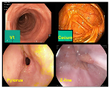 | Normal (V1/cecum/ pylorus/z-line) | 2800 | 1074 | 512 | 4386 |
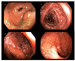 | Ulcerative Colitis | 948 | 598 | 252 | 1798 |
 | Polyps | 949 | 595 | 249 | 1793 |
 | Esophagitis | 948 | 546 | 263 | 1757 |
| Total | 5645 | 2813 | 1276 | 9734 |
| Model | Validation Set | Test Set | ||||||
|---|---|---|---|---|---|---|---|---|
| Accuracy | Precision | Recall | F1-Score | Accuracy | Precision | Recall | F1-Score | |
| FLATer | 0.9623 | 0.9647 | 0.9747 | 0.9697 | 0.9663 | 0.9640 | 0.9804 | 0.9721 |
| ViT-B/16 | 0.9206 | 0.9139 | 0.9212 | 0.9175 | 0.9169 | 0.9434 | 0.9162 | 0.9296 |
| DenseNet 121 | 0.9090 | 0.9473 | 0.8580 | 0.9004 | 0.9075 | 0.9792 | 0.8639 | 0.9179 |
| EfficientNetB0 | 0.8130 | 0.8425 | 0.7504 | 0.7938 | 0.8088 | 0.9075 | 0.7579 | 0.8260 |
| MobileNet V2 | 0.8844 | 0.9044 | 0.8488 | 0.8757 | 0.8911 | 0.9471 | 0.8665 | 0.9050 |
| ResNet18 | 0.8822 | 0.9044 | 0.8436 | 0.8730 | 0.8832 | 0.9489 | 0.8508 | 0.8972 |
| ResNet50 | 0.9153 | 0.9197 | 0.9022 | 0.9109 | 0.9060 | 0.9435 | 0.8966 | 0.9195 |
| ResNeXt50-32x4d | 0.9244 | 0.9475 | 0.8919 | 0.9188 | 0.9216 | 0.9729 | 0.8940 | 0.9318 |
| VGG16 | 0.9001 | 0.9106 | 0.8781 | 0.8940 | 0.9013 | 0.9443 | 0.8874 | 0.9150 |
| Xception | 0.8756 | 0.8710 | 0.8695 | 0.8702 | 0.8879 | 0.9355 | 0.8730 | 0.9032 |
| GoogLeNet | 0.8497 | 0.8803 | 0.7947 | 0.8353 | 0.8433 | 0.9338 | 0.7945 | 0.8586 |
| Sample Rate | Quantity | Accuracy | Precision | Recall | F1-Score |
|---|---|---|---|---|---|
| 20% | 817 | 0.9633 | 0.9607 | 0.9800 | 0.9702 |
| 40% | 1635 | 0.9645 | 0.9600 | 0.9830 | 0.9713 |
| 60% | 2453 | 0.9645 | 0.9670 | 0.9753 | 0.9711 |
| 80% | 3271 | 0.9633 | 0.9649 | 0.9755 | 0.9702 |
| 100% | 4089 | 0.9636 | 0.9645 | 0.9764 | 0.9704 |
| Model | Validation Set | Test Set | ||||||
|---|---|---|---|---|---|---|---|---|
| Accuracy | Precision | Recall | F1-Score | Accuracy | Precision | Recall | F1-Score | |
| FLATer | 0.9977 | 0.9978 | 0.9978 | 0.9978 | 0.9961 | 0.9960 | 0.9961 | 0.9960 |
| ViT-B/16 | 0.9839 | 0.9841 | 0.9844 | 0.9842 | 0.9895 | 0.9894 | 0.9894 | 0.9894 |
| DenseNet121 | 0.9448 | 0.9596 | 0.8803 | 0.9182 | 0.9594 | 0.9782 | 0.9032 | 0.9392 |
| EfficientNetB0 | 0.8712 | 0.8199 | 0.8440 | 0.8318 | 0.9045 | 0.8846 | 0.8554 | 0.8697 |
| MobileNetV2 | 0.9344 | 0.9618 | 0.8499 | 0.9024 | 0.9503 | 0.9692 | 0.8871 | 0.9263 |
| ResNet18 | 0.9103 | 0.9316 | 0.8112 | 0.8673 | 0.9215 | 0.9130 | 0.8537 | 0.8824 |
| ResNet50 | 0.9339 | 0.9635 | 0.8535 | 0.9051 | 0.9398 | 0.9554 | 0.8629 | 0.9068 |
| ResNeXt50-32x4d | 0.9500 | 0.9474 | 0.9091 | 0.9278 | 0.9503 | 0.9489 | 0.8956 | 0.9215 |
| VGG16 | 0.9097 | 0.9720 | 0.7635 | 0.8553 | 0.9149 | 0.9697 | 0.7773 | 0.8629 |
| Xception | 0.9563 | 0.9645 | 0.9172 | 0.9403 | 0.9516 | 0.9496 | 0.9150 | 0.9320 |
| GoogLeNet | 0.9086 | 0.8602 | 0.8910 | 0.8753 | 0.9346 | 0.9032 | 0.9106 | 0.9069 |
| Sample Rate | Quantity | Accuracy | Precision | Recall | F1-Score |
|---|---|---|---|---|---|
| 20% | 499 | 0.9980 | 0.9980 | 0.9979 | 0.9980 |
| 40% | 1000 | 0.9960 | 0.9961 | 0.9960 | 0.9960 |
| 60% | 1501 | 0.9967 | 0.9967 | 0.9967 | 0.9967 |
| 80% | 2002 | 0.9970 | 0.9970 | 0.9970 | 0.9970 |
| 100% | 2503 | 0.9972 | 0.9972 | 0.9972 | 0.9972 |
| Task | Model | Validation Set | Test Set | ||||||
|---|---|---|---|---|---|---|---|---|---|
| Accuracy | Precision | Recall | F1-Score | Accuracy | Precision | Recall | F1-Score | ||
| Binary Classification | FLATer | 0.9623 | 0.9647 | 0.9747 | 0.9697 | 0.9663 | 0.9640 | 0.9804 | 0.9721 |
| w/o residual block | 0.9366 | 0.9309 | 0.9373 | 0.9341 | 0.9350 | 0.9583 | 0.9319 | 0.9449 | |
| w/o spatial attention | 0.9470 | 0.9469 | 0.9425 | 0.9447 | 0.9491 | 0.9641 | 0.9503 | 0.9572 | |
| ViT backbone | 0.9206 | 0.9139 | 0.9212 | 0.9175 | 0.9169 | 0.9434 | 0.9162 | 0.9296 | |
| Ternary Classification | FLATer | 0.9977 | 0.9978 | 0.9978 | 0.9978 | 0.9961 | 0.9960 | 0.9961 | 0.9960 |
| w/o residual block | 0.9885 | 0.9889 | 0.9888 | 0.9888 | 0.9869 | 0.9870 | 0.9866 | 0.9867 | |
| w/o spatial attention | 0.9914 | 0.9916 | 0.9915 | 0.9916 | 0.9961 | 0.9960 | 0.9961 | 0.9960 | |
| ViT backbone | 0.9839 | 0.9841 | 0.9844 | 0.9842 | 0.9895 | 0.9894 | 0.9894 | 0.9894 | |
| Task | Model | Validation Set | Test Set | ||||||
|---|---|---|---|---|---|---|---|---|---|
| Accuracy | Precision | Recall | F1-Score | Accuracy | Precision | Recall | F1-Score | ||
| Binary Classification | FLATer | 0.9172 | 0.9363 | 0.9293 | 0.9328 | 0.9224 | 0.9427 | 0.9267 | 0.9347 |
| ResNeXt50 | 0.9068 | 0.9354 | 0.8654 | 0.8990 | 0.8934 | 0.9591 | 0.8586 | 0.9061 | |
| ViT | 0.8786 | 0.8887 | 0.8539 | 0.8710 | 0.8723 | 0.9238 | 0.8573 | 0.8893 | |
| Ternary Classification | FLATer | 0.9586 | 0.9602 | 0.9597 | 0.9597 | 0.9660 | 0.9655 | 0.9654 | 0.9654 |
| ResNeXt50 | 0.9356 | 0.9584 | 0.8550 | 0.9037 | 0.9450 | 0.9602 | 0.8750 | 0.9156 | |
| ViT | 0.8752 | 0.8534 | 0.7757 | 0.8127 | 0.8835 | 0.8419 | 0.7912 | 0.8157 | |
| Task | Model | Validation Set | Test Set | ||||||
|---|---|---|---|---|---|---|---|---|---|
| Accuracy | Precision | Recall | F1-Score | Accuracy | Precision | Recall | F1-Score | ||
| Binary Classification | 12-layers | 0.9623 | 0.9647 | 0.9747 | 0.9697 | 0.9663 | 0.9640 | 0.9804 | 0.9721 |
| 6-layers | 0.9520 | 0.9718 | 0.9500 | 0.9607 | 0.9389 | 0.9610 | 0.9359 | 0.9483 | |
| 4-layers | 0.9250 | 0.9494 | 0.9281 | 0.9386 | 0.9279 | 0.9565 | 0.9215 | 0.9387 | |
| Ternary Classification | 12-layers | 0.9977 | 0.9978 | 0.9978 | 0.9978 | 0.9961 | 0.9960 | 0.9961 | 0.9960 |
| 6-layers | 0.9896 | 0.9902 | 0.9899 | 0.9899 | 0.9948 | 0.9948 | 0.9946 | 0.9947 | |
| 4-layers | 0.9724 | 0.9742 | 0.9731 | 0.9731 | 0.9817 | 0.9822 | 0.9813 | 0.9814 | |
Disclaimer/Publisher’s Note: The statements, opinions and data contained in all publications are solely those of the individual author(s) and contributor(s) and not of MDPI and/or the editor(s). MDPI and/or the editor(s) disclaim responsibility for any injury to people or property resulting from any ideas, methods, instructions or products referred to in the content. |
© 2023 by the authors. Licensee MDPI, Basel, Switzerland. This article is an open access article distributed under the terms and conditions of the Creative Commons Attribution (CC BY) license (https://creativecommons.org/licenses/by/4.0/).
Share and Cite
Wu, S.; Zhang, R.; Yan, J.; Li, C.; Liu, Q.; Wang, L.; Wang, H. High-Speed and Accurate Diagnosis of Gastrointestinal Disease: Learning on Endoscopy Images Using Lightweight Transformer with Local Feature Attention. Bioengineering 2023, 10, 1416. https://doi.org/10.3390/bioengineering10121416
Wu S, Zhang R, Yan J, Li C, Liu Q, Wang L, Wang H. High-Speed and Accurate Diagnosis of Gastrointestinal Disease: Learning on Endoscopy Images Using Lightweight Transformer with Local Feature Attention. Bioengineering. 2023; 10(12):1416. https://doi.org/10.3390/bioengineering10121416
Chicago/Turabian StyleWu, Shibin, Ruxin Zhang, Jiayi Yan, Chengquan Li, Qicai Liu, Liyang Wang, and Haoqian Wang. 2023. "High-Speed and Accurate Diagnosis of Gastrointestinal Disease: Learning on Endoscopy Images Using Lightweight Transformer with Local Feature Attention" Bioengineering 10, no. 12: 1416. https://doi.org/10.3390/bioengineering10121416
APA StyleWu, S., Zhang, R., Yan, J., Li, C., Liu, Q., Wang, L., & Wang, H. (2023). High-Speed and Accurate Diagnosis of Gastrointestinal Disease: Learning on Endoscopy Images Using Lightweight Transformer with Local Feature Attention. Bioengineering, 10(12), 1416. https://doi.org/10.3390/bioengineering10121416