


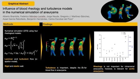
Influence of Blood Rheology and Turbulence Models in the Numerical Simulation of Aneurysms

 ,
,
Abstract
:
1. Introduction
2. Materials and Methods
2.1. Governing Equations
2.2. Transport Equations for the Standard Model
2.3. Fluid–Solid Interaction (FSI)
2.4. Boundary Conditions
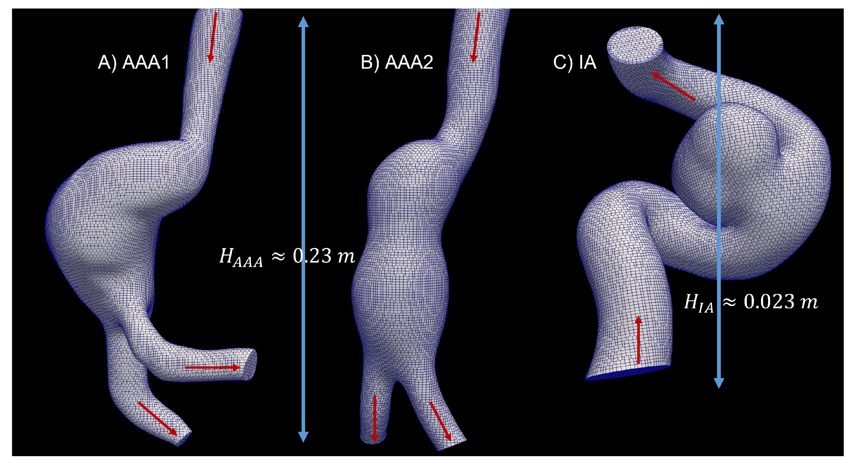
2.5. 3D Model
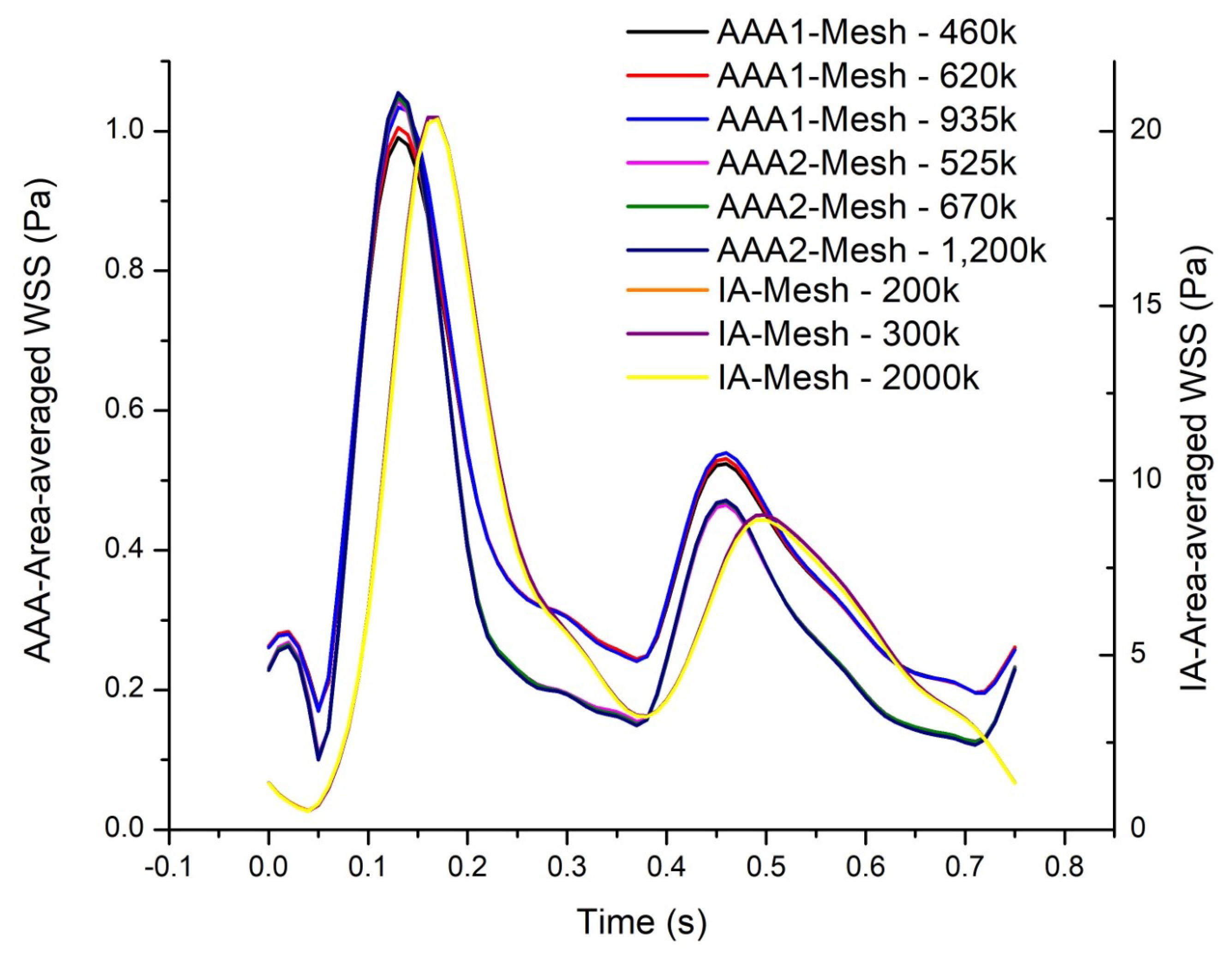
2.6. Grid Generation
3. Results
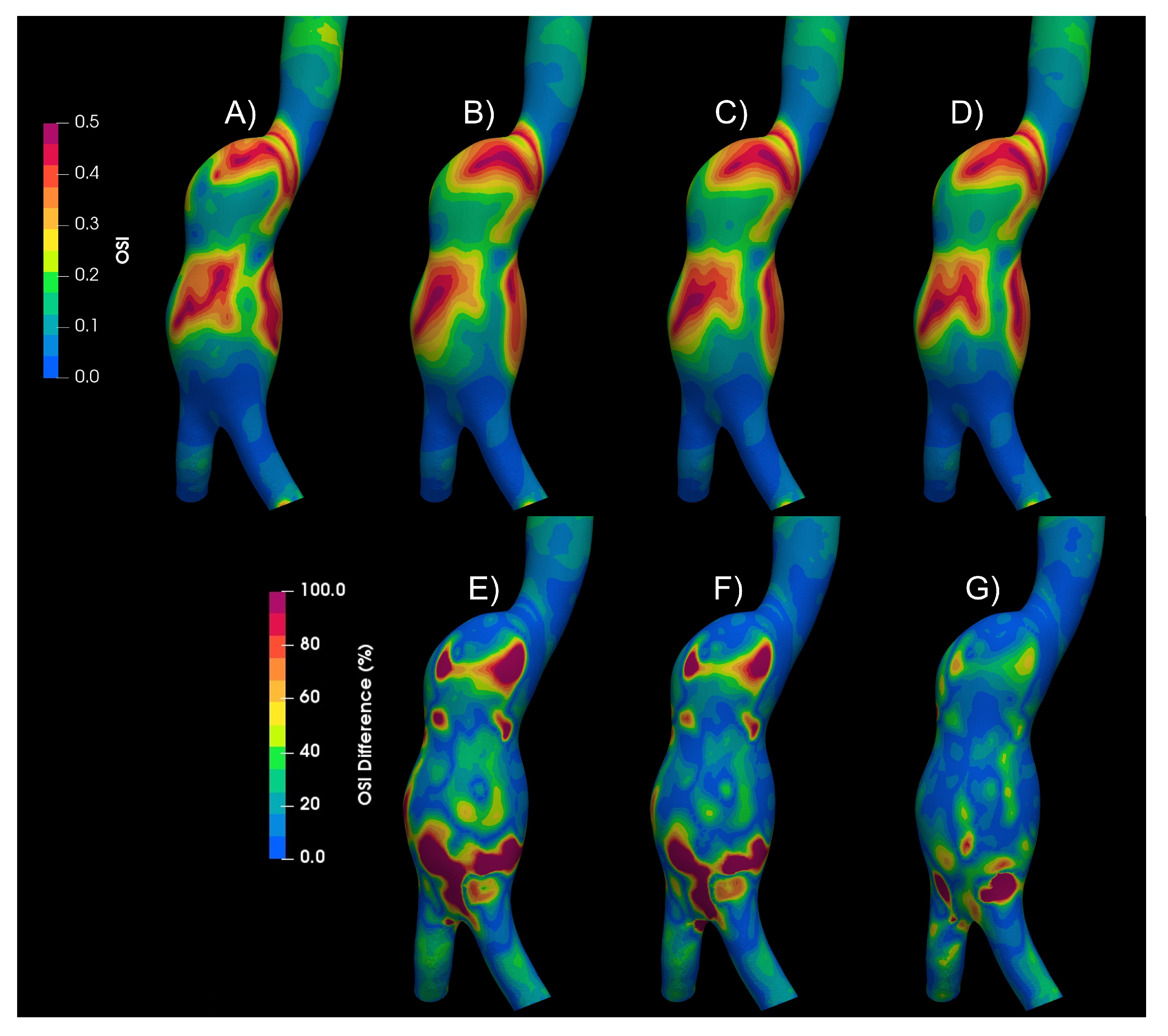
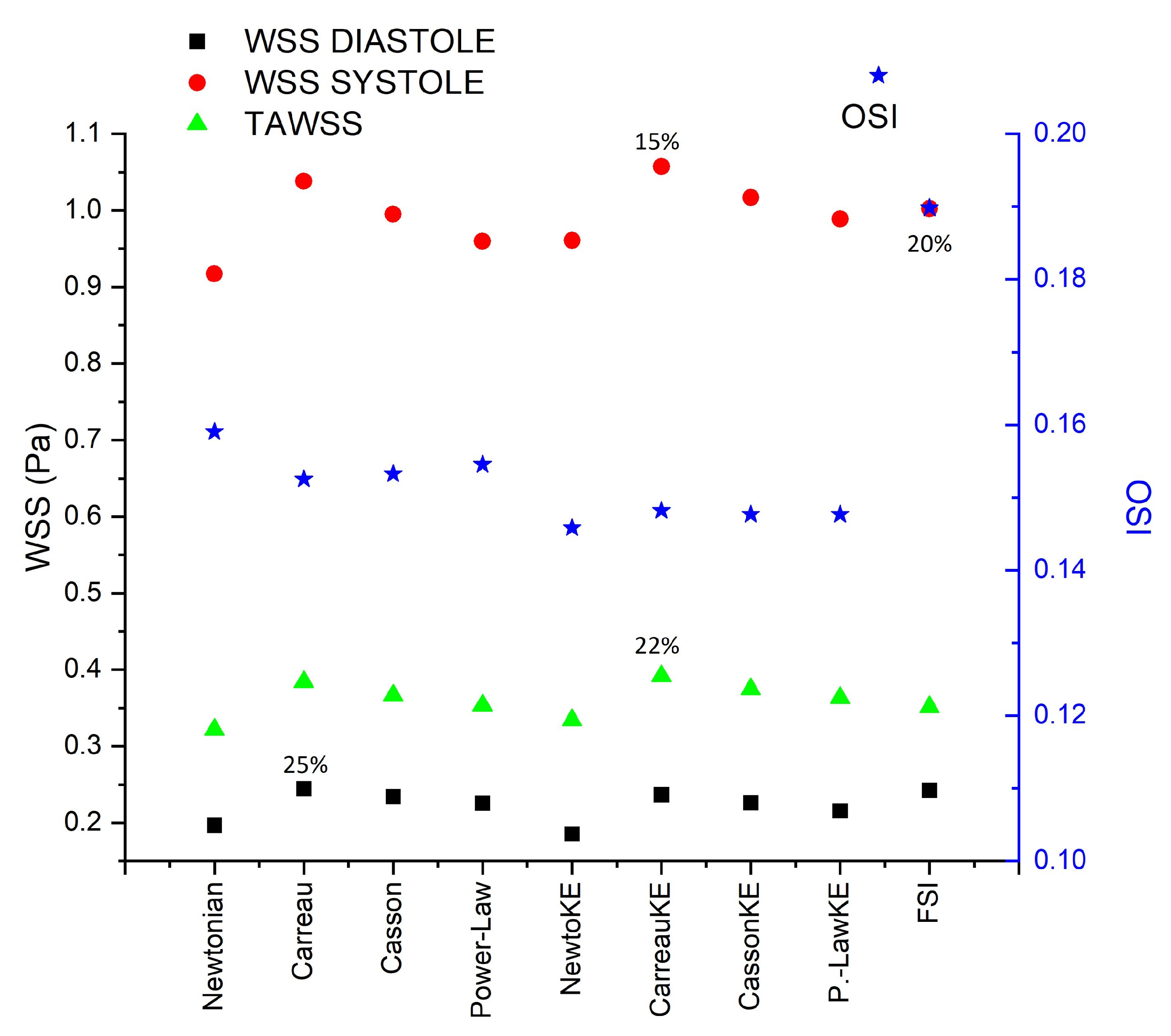
3.1. Rheology
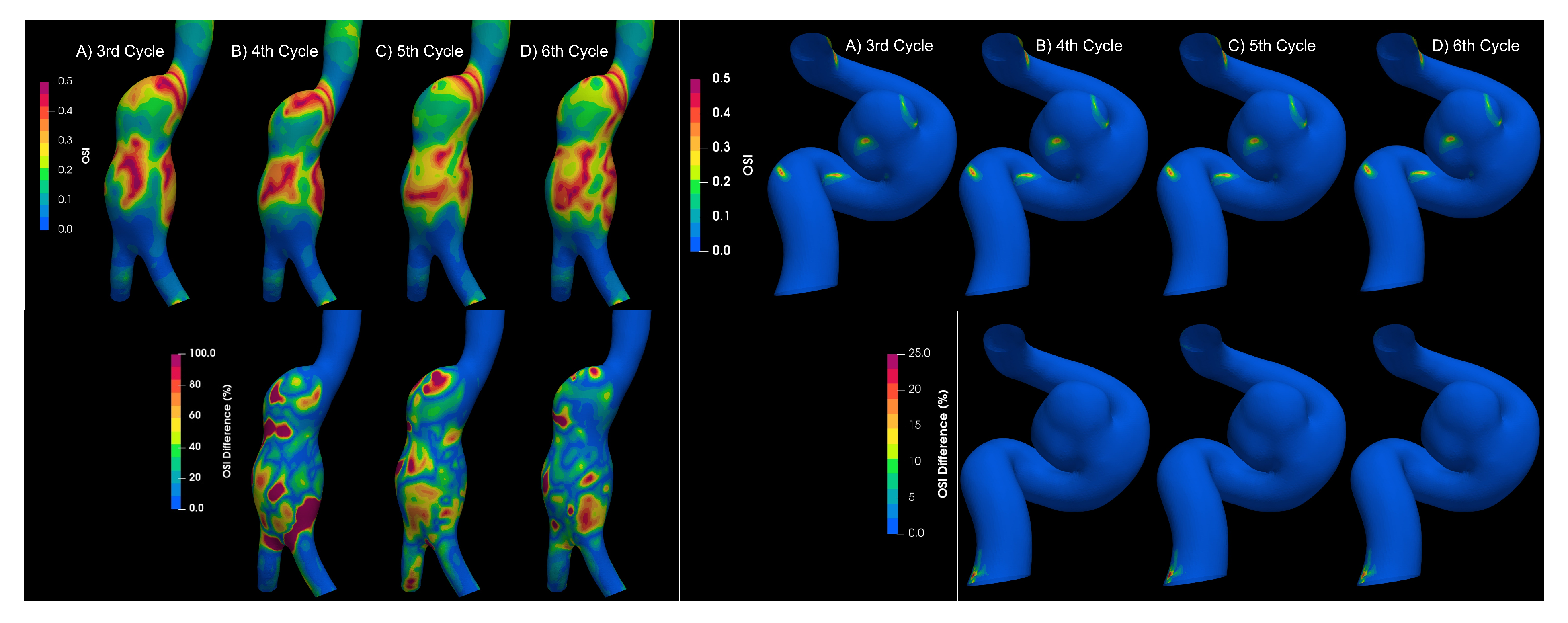
3.2. Turbulence
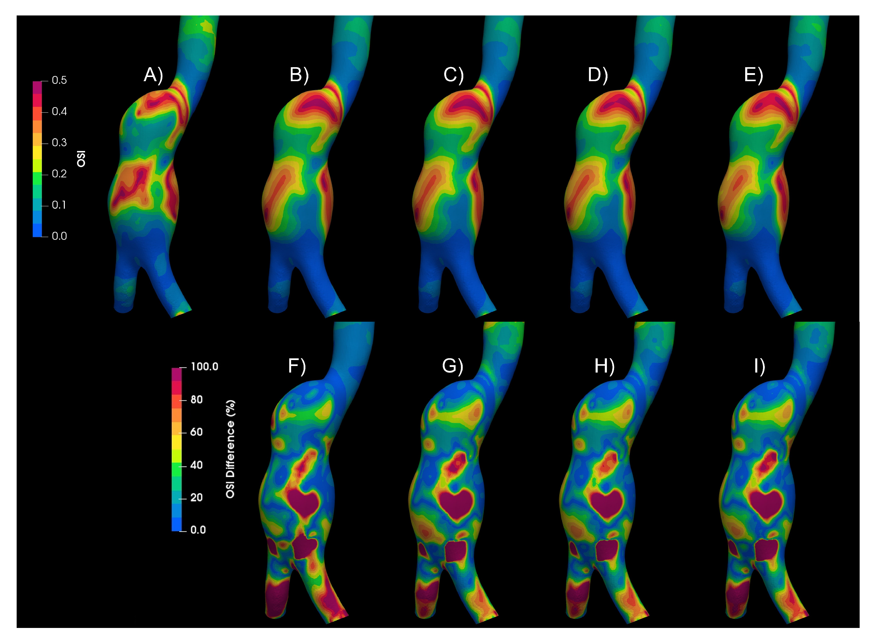
3.3. Fluid–Solid Interaction (FSI)
4. Discussion
Author Contributions
Funding
Institutional Review Board Statement
Informed Consent Statement
Data Availability Statement
Acknowledgments
Conflicts of Interest
Abbreviations
| FSI | Fluid–structure interaction |
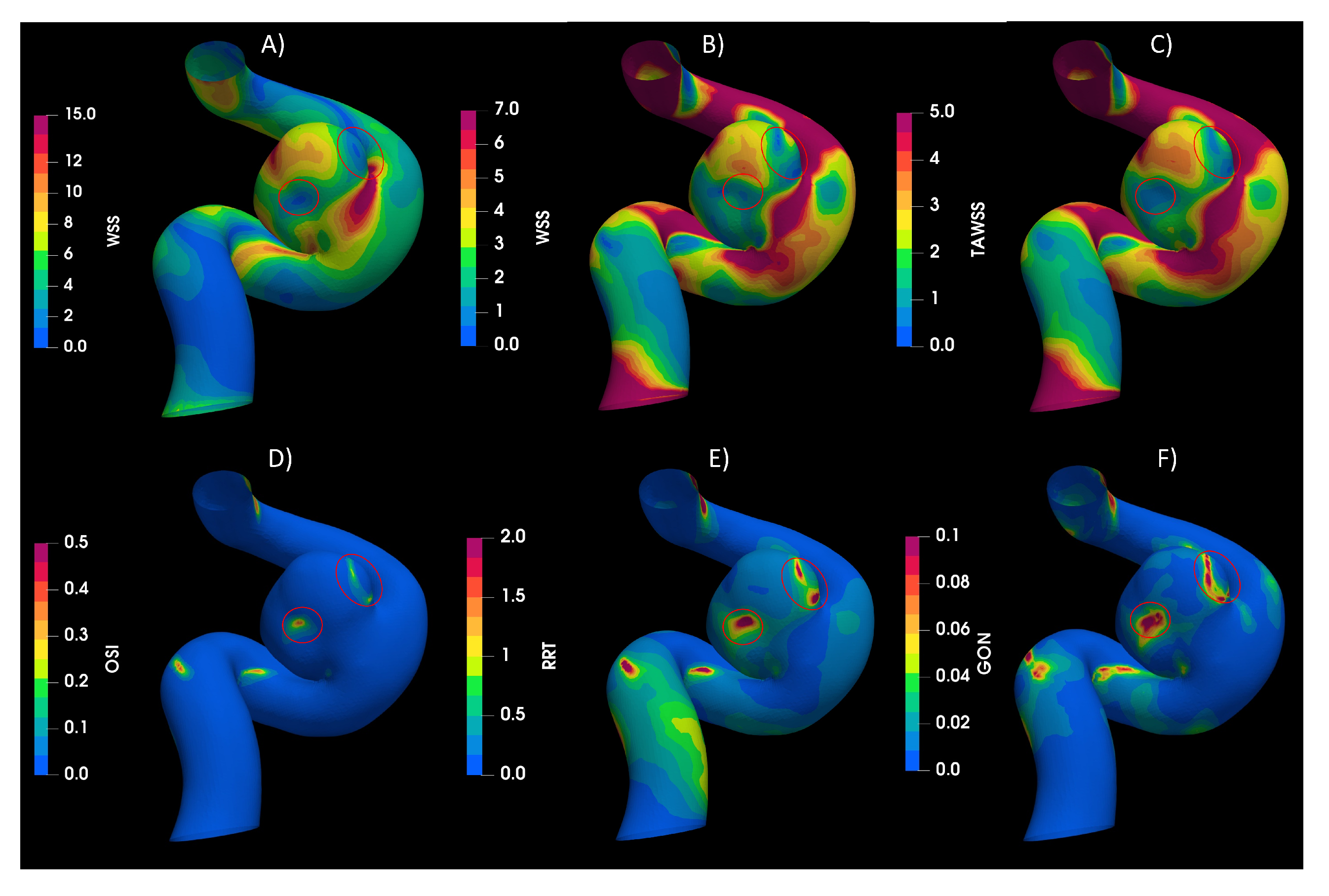
| OSI | Oscillatory shear index |
| GON | Gradient oscillatory number |
| CFD | Computational fluid dynamic |
| AAA | Aortic Aneurysms |
| IA | Intracranial Aneurysm |
| WSS | Wall shear stresss |
| TAWSS | Time-Averaged Wall Shear Stress |
| RRT | Relative Residence Time |
| DSA | Digital Substraction Angiography |
References
- Alam, M.; Mut, F.; Cebral, J.R.; Seshaiyer, P. Quantification of the Rupture Potential of Patient-Specific Intracranial Aneurysms under Contact Constraints. Bioengineering 2021, 8, 149. [Google Scholar] [CrossRef] [PubMed]
- Le Bras, A.; Boustia, F.; Janot, K.; Le Pabic, E.; Ouvrard, M.; Fougerou-Leurent, C.; Ferre, J.C.; Gauvrit, J.Y.; Eugene, F. Rehearsals using patient-specific 3D-printed aneurysm models for simulation of endovascular embolization of complex intracranial aneurysms: 3D SIM study. J. Neuroradiol. 2023, 50, 86–92. [Google Scholar] [CrossRef] [PubMed]
- Epshtein, M.; Korin, N. Mapping the Transport Kinetics of Molecules and Particles in Idealized Intracranial Side Aneurysms. Sci. Rep. 2018, 8, 8528. [Google Scholar] [CrossRef] [PubMed]
- Sheikh, M.A.A.; Shuib, A.S.; Mohyi, M.H.H. A review of hemodynamic parameters in cerebral aneurysm. Interdiscip. Neurosurg. 2020, 22, 100716. [Google Scholar] [CrossRef]
- Longo, M.; Granata, F.; Racchiusa, S.; Mormina, E.; Grasso, G.; Longo, G.M.; Garufi, G.; Salpietro, F.M.; Alafaci, C. Role of Hemodynamic Forces in Unruptured Intracranial Aneurysms: An Overview of a Complex Scenario. World Neurosurg. 2017, 105, 632–642. [Google Scholar] [CrossRef] [PubMed]
- Carty, G.; Chatpun, S.; Espino, D.M. Modeling Blood Flow Through Intracranial Aneurysms: A Comparison of Newtonian and Non-Newtonian Viscosity. J. Med. Biol. Eng. 2016, 36, 396–409. [Google Scholar] [CrossRef]
- Lee, C.; Zhang, Y.; Takao, H.; Murayama, Y.; Qian, Y. A fluid–structure interaction study using patient-specific ruptured and unruptured aneurysm: The effect of aneurysm morphology, hypertension and elasticity. J. Biomech. 2013, 46, 2402–2410. [Google Scholar] [CrossRef]
- Han, S.; Schirmer, C.M.; Modarres-Sadeghi, Y. A reduced-order model of a patient-specific cerebral aneurysm for rapid evaluation and treatment planning. J. Biomech. 2020, 103, 109653. [Google Scholar] [CrossRef]
- Poelma, C.; Watton, P.N.; Ventikos, Y. Transitional flow in aneurysms and the computation of haemodynamic parameters. J. R. Soc. Interface 2015, 12, 20141394. [Google Scholar] [CrossRef]
- Moradicheghamahi, J.; Sadeghiseraji, J.; Jahangiri, M. Numerical solution of the Pulsatile, non-Newtonian and turbulent blood flow in a patient specific elastic carotid artery. Int. J. Mech. Sci. 2019, 150, 393–403. [Google Scholar] [CrossRef]
- Ascolese, M.; Farina, A.; Fasano, A. The Fåhræus-Lindqvist effect in small blood vessels: How does it help the heart? J. Biol. Phys. 2019, 45, 379–394. [Google Scholar] [CrossRef] [PubMed]
- Abbasian, M.; Shams, M.; Valizadeh, Z.; Moshfegh, A.; Javadzadegan, A.; Cheng, S. Effects of different non-Newtonian models on unsteady blood flow hemodynamics in patient-specific arterial models with in-vivo validation. Comput. Methods Programs Biomed. 2020, 186, 105185. [Google Scholar] [CrossRef]
- Abugattas, C.; Aguirre, A.; Castillo, E.; Cruchaga, M. Numerical study of bifurcation blood flows using three different non-Newtonian constitutive models. Appl. Math. Model. 2020, 88, 529–549. [Google Scholar] [CrossRef]
- Fukazawa, K.; Ishida, F.; Umeda, Y.; Miura, Y.; Shimosaka, S.; Matsushima, S.; Taki, W.; Suzuki, H. Using Computational Fluid Dynamics Analysis to Characterize Local Hemodynamic Features of Middle Cerebral Artery Aneurysm Rupture Points. World Neurosurg. 2015, 83, 80–86. [Google Scholar] [CrossRef]
- Qiu, Y.; Wang, J.; Zhao, J.; Wang, T.; Zheng, T.; Yuan, D. Association Between Blood Flow Pattern and Rupture Risk of Abdominal Aortic Aneurysm Based on Computational Fluid Dynamics. Eur. J. Vasc. Endovasc. Surg. 2022, 64, 155–164. [Google Scholar] [CrossRef]
- Perdikaris, P.; Insley, J.A.; Grinberg, L.; Yu, Y.; Papka, M.E.; Karniadakis, G.E. Visualizing multiphysics, fluid-structure interaction phenomena in intracranial aneurysms. Parallel Comput. 2016, 55, 9–16. [Google Scholar] [CrossRef] [PubMed]
- Wang, X.; Li, X. Computational simulation of aortic aneurysm using FSI method: Influence of blood viscosity on aneurismal dynamic behaviors. Comput. Biol. Med. 2011, 41, 812–821. [Google Scholar] [CrossRef] [PubMed]
- Jiang, Y.; Lu, G.; Ge, L.; Huang, L.; Wan, H.; Wan, J.; Zhang, X. Rupture point hemodynamics of intracranial aneurysms: Case report and literature review. Ann. Vasc. Surg.-Brief Rep. Innov. 2021, 1, 100022. [Google Scholar] [CrossRef]
- OpenFOAM|Free CFD Software|The OpenFOAM Foundation—openfoam.org. Available online: https://openfoam.org/ (accessed on 9 September 2023).
- Bilgi, C.; Atalik, K. Numerical investigation of the effects ofblood rheology and wall elasticity in abdominal aortic aneurysm under pulsatile flow conditions. Biorheology 2019, 56, 51–71. [Google Scholar] [CrossRef]
- Kim, S.; Cho, Y.I.; Jeon, A.H.; Hogenauer, B.; Kensey, K.R. A new method for blood viscosity measurement. J. Non-Newton. Fluid Mech. 2000, 94, 47–56. [Google Scholar] [CrossRef]
- Carvalho, M.V.P.; Lobosco, R.J.; Júnior, G.B.L. Rheological Analysis of Blood Flow in the Bifurcation of Carotid Artery with OpenFOAM. In Proceedings of the 4th Brazilian Technology Symposium (BTSym’18), Campinas, SP, Brazil, 23–25 October 2018; Iano, Y., Arthur, R., Saotome, O., Vieira Estrela, V., Loschi, H.J., Eds.; Springer International Publishing: Cham, Switzerland, 2019; pp. 223–230. [Google Scholar]
- Johnston, B.M.; Johnston, P.R.; Corney, S.; Kilpatrick, D. Non-Newtonian blood flow in human right coronary arteries: Steady state simulations. J. Biomech. 2004, 37, 709–720. [Google Scholar] [CrossRef] [PubMed]
- Bazilevs, Y.; Hsu, M.C.; Zhang, Y.; Wang, W.; Kvamsdal, T.; Hentschel, S.; Isaksen, J.G. Computational vascular fluid-structure interaction: Methodology and application to cerebral aneurysms. Biomech. Model. Mechanobiol. 2010, 9, 481–498. [Google Scholar] [CrossRef]
- Torii, R.; Oshima, M.; Kobayashi, T.; Takagi, K.; Tezduyar, T.E. Fluid-structure interaction modeling of a patient-specific cerebral aneurysm: Influence of structural modeling. Comput. Mech. 2008, 43, 151–159. [Google Scholar] [CrossRef]
- Isaksen, J.G.; Bazilevs, Y.; Kvamsdal, T.; Zhang, Y.; Kaspersen, J.H.; Waterloo, K.; Romner, B.; Ingebrigtsen, T. Determination of wall tension in cerebral artery aneurysms by numerical simulation. Stroke 2008, 39, 3172–3178. [Google Scholar] [CrossRef] [PubMed]
- Banerjee, M.K.; Ganguly, R.; Datta, A. Effect of Pulsatile Flow Waveform and Womersley Number on the Flow in Stenosed Arterial Geometry. ISRN Biomath. 2012, 2012, 1–17. [Google Scholar] [CrossRef]
- Escobar-del Pozo, C.; Brambila-Solrzano, A. Aneurysms flow numerical simulation CFD-Evaluation of rheological models. Mendeley Data. 2021. [Google Scholar] [CrossRef]
- Munarriz, P.; Gómez, P.A.; Paredes, I.; Castaño-Leon, A.M.; Cepeda, S.; Lagares, A. Basic Principles of Hemodynamics and Cerebral Aneurysms. World Neurosurg. 2016, 88, 311–319. [Google Scholar] [CrossRef]
- Meng, H.; Tutino, V.; Xiang, J.; Siddiqui, A. High WSS or Low WSS? Complex interactions of hemodynamics with intracranial aneurysm initiation, growth, and rupture: Toward a unifying hypothesis. Am. J. Neuroradiol. 2014, 35, 1254–1262. [Google Scholar] [CrossRef]
- Hershey, D.; Im, C.S. Critical reynolds number for sinusoidal flow of water in rigid tubes. AIChE J. 1968, 14, 807–809. [Google Scholar] [CrossRef]
- Nerem, R.M.; Seed, W.A. An in vivo study of aortic flow disturbances. Cardiovasc. Res. 1972, 6, 1–14. [Google Scholar] [CrossRef]
- Pratumwal, Y.; Limtrakarn, W.; Muengtaweepongsa, S.; Phakdeesan, P.; Duangburong, S.; Eiamaram, P.; Intharakham, K. Whole blood viscosity modeling using power law, Casson, and Carreau Yasuda models integrated with image scanningU-tube viscometer technique. Songklanakarin J. Sci. Technol. (SJST) 2017, 39, 5. [Google Scholar] [CrossRef]


| MODEL | PARAMETERS | |
|---|---|---|
| Newtonian | Pa.s | [20] |
| Power law | , | [21] |
| Casson | Pa.s, Pa | [22] |
| Carreau | Pa.s, s Pa.s, | [23] |
| Strain Rate | AAA1 | AAA2 | IA |
|---|---|---|---|
| Artery Wall | 125 | 97 | 1888 |
| Aneurysm Wall | 89 | 73 | 1480 |
| Artery Body | 19 | 22 | 502 |
| Aneurysm Body | 15 | 20 | 388 |
Disclaimer/Publisher’s Note: The statements, opinions and data contained in all publications are solely those of the individual author(s) and contributor(s) and not of MDPI and/or the editor(s). MDPI and/or the editor(s) disclaim responsibility for any injury to people or property resulting from any ideas, methods, instructions or products referred to in the content. |
© 2023 by the authors. Licensee MDPI, Basel, Switzerland. This article is an open access article distributed under the terms and conditions of the Creative Commons Attribution (CC BY) license (https://creativecommons.org/licenses/by/4.0/).
Share and Cite
Brambila-Solórzano, A.; Méndez-Lavielle, F.; Naude, J.L.; Martínez-Sánchez, G.J.; García-Rebolledo, A.; Hernández, B.; Escobar-del Pozo, C. Influence of Blood Rheology and Turbulence Models in the Numerical Simulation of Aneurysms. Bioengineering 2023, 10, 1170. https://doi.org/10.3390/bioengineering10101170
Brambila-Solórzano A, Méndez-Lavielle F, Naude JL, Martínez-Sánchez GJ, García-Rebolledo A, Hernández B, Escobar-del Pozo C. Influence of Blood Rheology and Turbulence Models in the Numerical Simulation of Aneurysms. Bioengineering. 2023; 10(10):1170. https://doi.org/10.3390/bioengineering10101170
Chicago/Turabian StyleBrambila-Solórzano, Alberto, Federico Méndez-Lavielle, Jorge Luis Naude, Gregorio Josué Martínez-Sánchez, Azael García-Rebolledo, Benjamín Hernández, and Carlos Escobar-del Pozo. 2023. "Influence of Blood Rheology and Turbulence Models in the Numerical Simulation of Aneurysms" Bioengineering 10, no. 10: 1170. https://doi.org/10.3390/bioengineering10101170
APA StyleBrambila-Solórzano, A., Méndez-Lavielle, F., Naude, J. L., Martínez-Sánchez, G. J., García-Rebolledo, A., Hernández, B., & Escobar-del Pozo, C. (2023). Influence of Blood Rheology and Turbulence Models in the Numerical Simulation of Aneurysms. Bioengineering, 10(10), 1170. https://doi.org/10.3390/bioengineering10101170