Article

Supercritical Flow over a Submerged Vertical Negative Step

by
Eugene Retsinis
* and
Panos Papanicolaou
School of Civil Engineering, National Technical University of Athens, 9 Iroon Polytexneiou St., 15780 Athens, Greece
*
Author to whom correspondence should be addressed.
Hydrology 2022, 9(5), 74; https://doi.org/10.3390/hydrology9050074
Submission received: 28 March 2022 / Revised: 18 April 2022 / Accepted: 26 April 2022 / Published: 28 April 2022

Abstract

:
The transition from supercritical to subcritical flow around a fully submerged abrupt negative step in a horizontal rectangular open channel has been investigated. In a laboratory experiment the one-dimensional energy and the momentum conservation equations were studied by means of depth and pressure measurements by piezometers installed along the bottom and the step face. Froude number varied in the range 1.9 to 5.8 while the step height to critical depth ratio was in the range 1.34 to 2.56. The results are presented in dimensionless form using mainly a characteristic length scale that is the sum of critical depth and step height and the Froude number of the supercritical flow upstream. Five different types of rapidly varying flow are observed when the subcritical downstream tailwater depth varied. The supercritical water jet at the top of the step either strikes the bottom downstream of the step when the maximum pressure head is greater, or moves to the surface of the flow when it is lower than tailwater depth, and the separation of the two flow regimes occurs when the tailwater depth to the characteristic length scale is around 1.05. The normalized energy loss and a closure parameter for the momentum equation are presented in dimensionless diagrams for practical use by the design engineer. Finally, the one-dimensional equations of motion including Boussinesq terms are solved numerically and the results found are congruent to the experimental findings.

1. Introduction

Stilling basins are designed to dissipate the kinetic energy of the flow by means of hydraulic jumps formed in them, for which a thorough investigation of the physical and numerical study is reported in [1]. In several cases an abrupt forward facing (negative) step is introduced to stabilize the jump, so that it is not swept away from the basin. The transition from supercritical to subcritical flow at an abrupt negative step affects the design and construction of a stilling basin. The design usually includes determination of the step height, the required tailwater water elevation, an adequate basin length and all necessary structures in it such as blocks, end sill, etc. Submerged negative steps can also be met in river training works, in canals conveying water, as well as in natural streams. Engineers and scientists have been studying the flow of submerged steps in the laboratory for a long time, measuring mainly the flow depths and pressure distribution at the bottom and the step face, and trying to correlate the flow parameters to energy and momentum conservation, as well as to the various flow profiles that appear there.
In laboratory experiments the flow is usually controlled by a sluice gate upstream, and a sharp crested overflow downstream of the step. Five different rapidly varying flow profiles have been observed around a step with supercritical flow upstream and subcritical downstream [2,3,4], namely minimum B-jump, B-jump, wave-train, wave-jump and A-jump (Figure 1). Minimum B-jump (Figure 1i) is the hydraulic jump at the toe of the step, B-jump (Figure 1ii) is the submerged jump downstream of the step, wave-train (Figure 1iii) is the surface jet-type flow without formation of a hydraulic jump, wave-jump (Figure 1iv) is the flow of an ascending jet forming a standing wave downstream of the step, before it dives and results in a submerged hydraulic jump, and A-jump (Figure 1v) is the flow where the hydraulic jump is formed upstream of the step. These profiles appear with the above sequence if one increases the downstream tailwater depth continuously.
Several researchers in the past have studied the transition from supercritical to subcritical flow over a fully submerged negative (abrupt or rounded) step by experiments. Several authors [2,3,4,5,6,7,8,9,10,11] have investigated the influence of the pressure distribution at the face of the step of different jump types in order to obtain closure of the one-dimensional momentum equation. Velocity and shear stress distribution was measured [12] at the channel bottom using a Preston tube. In some cases the flow type alternated between B-jump, wave-train and wave-jump every once in a while [4,13,14], thus resulting in varying velocity and pressure fields. Standard deviation of pressure fluctuations at the channel bottom axis was measured by [15], while published experimental results of jumps at an abrupt drop with subcritical and supercritical flow conditions upstream have also been reported [16]. The presence of roughness elements inside a channel with an abrupt drop reduced the pressure forces on the bottom axis of the channel [17,18], if compared to the developed pressure either from the classical hydraulic jump or inside a smooth channel with drop. Also, for upstream Froude number greater than eight, the relative height of the step to upstream depth d/y1 does not seem to affect the energy loss [5], while the energy dissipation of the jump [6] is higher in the case of a channel with negative step, if compared to the energy loss in a channel with a positive step. The wave-jump type flow was found to dissipate the energy more efficiently than the classical hydraulic jump [7,19], while inclined channels under the presence of negative or positive step with sharp crested B-jumps resulted in higher energy dissipation than A-jumps [20]. The different flow profiles developed in sloping rectangular open channels with an abrupt drop have also been investigated [21], while the highest energy loss was observed in B-jump, if compared to the minimum B-jump and the A-jump [22]. The energy loss was reported [23] in dimensionless form, while jumps formed at a negative step are more stable, energy dissipative efficient and more compact [24], if compared to the jumps appearing in positive steps.
Regarding numerical modeling of the flow in the presence of an abrupt step, the B-jump was studied [25] in an open channel 0.4 m wide with a 9.7 cm abrupt drop high for upstream Froude numbers 1.21 and 1.4. The Reynolds-Averaged Navier Stokes (RANS) equations were solved using the ANSYS-FLUENT commercial software with the finite volume method to compute the free surface profile and the time-averaged velocity field. The B-jump, wave-jump and A-jump in an open channel 2 m long and 0.4 m wide with abrupt drops 3.20 and 6.52 cm high, for Froude number in the range 2.8–3.9, have been studied [26] using Smoothed Particle Hydrodynamics (SPH) to discretize the Navier Stokes equations along with k-ε turbulence model. The results regarded the computation of the instantaneous velocity and vorticity fields.
Systematic pressure measurements have not been reported to date in the area of an abrupt drop in an open channel hence, pressure distribution cannot be linked to the linear characteristics of the flow. Energy losses and momentum equation balance have not been reported conclusively around a step with supercritical flow upstream, which is a result due to lack of use of the appropriate dimensionless representation of them. The aim of the present work is to investigate the rapidly varying flow in a horizontal rectangular open channel with the presence of a fully submerged abrupt negative step, with supercritical flow upstream and subcritical downstream. To obtain it we performed systematic measurements of the linear flow characteristics as well as the pressure at the bottom and face of the step, for supercritical flow upstream with Froude number up to about 6. From these measurements the conditions under which different flow patterns appear, as well as other aspects of the flow, such as the closure of the one-dimensional momentum and energy loss equations will be investigated, and the results will be presented in dimensionless form. The Saint Venant equations will be solved in one dimension including Boussinesq terms that have been usually omitted in the past, to evaluate some of the experimental findings.

2. Theory

The flow under investigation (Figure 2) is that around a vertical forward facing (negative) step where the flow upstream is supercritical and downstream subcritical. The parameters involved are the flow rate per unit width q, the step height d, the upstream and downstream depths y1 and y2 and mean velocities V1 and V2, respectively. Two parameters that are important in the description of the flow are the critical depth yc = (q2/g)1/3 and the Froude number of the supercritical flow upstream of the step Fr1 = V1/(gy1)1/2, g being the gravitational acceleration.
Let us study the flow theoretically using the one-dimensional momentum and energy conservation equations [27]. We apply the one-dimensional momentum equation along the main flow direction per unit width, in the control volume between upstream Cross Section 1 with supercritical flow and downstream Cross Section 2 with subcritical flow, and depths y1 and y2, respectively, to get
1 2 gy 1 2 + kgd ( y 1 + d / 2 ) 1 2 gy 2 2 = q ( V 2 V 1 )
In Equation (1) we assume that the velocity is uniform at Cross Section 1 and Section 2, the shear stresses at the wall and the bottom of the channel can be neglected, and the pressure distribution at the face of the step is hydrostatic hence, F1 = (gy12)/2, F2 = (gy22)/2 and Fs = kgd(y1 + d/2). To make Equation (1) valid, the second term on the left that corresponds to force on step face ρgd(y1 + d/2) from the hydrostatic pressure distribution with pressure ρgy1 at the top and ρg(y1 + d) at the bottom must be multiplied by a correction factor k, defined to be the ratio of the real pressure that is due to the curvature of the streamlines near the step, to the anticipated hydrostatic one at the middle of the step ρg(y1 + d/2) [3].
If the flow rate q and depths y1 and y2 are known, solving Equation (1) for k we get
k = q ( V 2 V 1 ) 1 2 g ( y 1 2 y 2 2 ) gd ( y 1 + d 2 )
Equation (2) holds if the flow depth at the step is y1, in other words for all types of flow but A-jump. For the latter case the term in the denominator must be replaced by gd(y2 − d/2).
The energy loss ΔH at the step is computed from the one-dimensional energy equation assuming known depths and flow rate, and uniform velocity at Cross Section 1 and Section 2.
Δ H = H 1 H 2 = d + y 1 + V 1 2 / 2 g y 2 V 2 2 / 2 g
where H1 and H2, are the energy heads at Cross Section 1 and Section 2, respectively, considering uniform velocity distributions.

3. Experiments

3.1. Setup and Procedure

Experiments were carried out at the Laboratory of Applied Hydraulics of the School of Civil Engineering at the National Technical University of Athens, Greece. The open channel used is 10.50 m long with rectangular cross section 0.255 m wide × 0.50 m deep is shown in Figure 3, and was equipped with a sluice gate upstream and a thin crested weir at downstream end. The section of the channel where measurements were taken has been modified to accommodate the experiments. The steel, nontransparent bottom has been replaced with Lucite with a row of piezometers attached to it, and the vertical side glass walls were replaced with new ones with improved optical properties.
The water supply was obtained via a recirculation system that consists of a 3 kW pump with variable speed motor and maximum discharge capacity of 40 L/s at 5 m head, which is connected to a 2.65 m3 water tank at the downstream end of the channel. Water was pumped to the upstream end of the channel through a PVC pipe of nominal diameter 0.2 m. The flowrate was measured with an ultrasonic flow meter of 2–5% accuracy, attached in the horizontal PVC pipe that flowed full about 10 pipe diameters downstream of the pump. A screen system at the entrance of the water in the channel was used to dissipate the kinetic energy of the inflow and reduce waves from agitation, upstream of the sluice gate.
A downstream facing vertical step 10.3 cm high and 1 m long made of Lucite was placed 4.85 m upstream of the channel end. The vertical sluice gate was positioned 0.35 m upstream of the step face, in order to control the flow from upstream. Ten piezometers were placed in the middle of the step and three along the middle of the step face. Twenty-one piezometers were placed along the middle of the Lucite bottom downstream of the step. The piezometers were de-aerated during the course of the experiment, once the step was submerged in the flow.
The flow was controlled with the vertical sluice gate and supercritical flow was obtained on the step surface at the desired inflow Froude number upstream from the drop. Downstream, the flow was controlled with a vertical sharp crested weir at the end of the channel, and the depth was adjusted to the desired level. Once the supercritical flow conditions were set upstream of the drop, the rapidly varying flow around it was adjusted by the tailwater depth. The depth of flow was measured using a point gauge and from the piezometers far downstream of the step, where the flow was parallel to the bottom.
The experimental procedure was as follows. The pump was set to the desired flow rate adjusted by the variable speed motor and measured with the ultrasonic flow meter, then the channel was filled with water above the step, keeping the end weir at the appropriate elevation. The piezometers were de-aerated and the supercritical flow upstream of the drop was adjusted to the desired inflow Froude number with the sluice gate opening. Then, the flow conditions downstream of the submerged step were adjusted with the end weir to the desired type of flow. Increasing the weir height gradually, the flow was set from minimum B-jump to B-jump, to wave-train, to (standing) wave-jump, to A-jump. The flow depths were measured with a point gauge with accuracy ±0.0001 m. The supercritical flow depth, y1, was measured at a distance 3 y1 upstream of the drop, while the tailwater subcritical depth y2 was measured at a distance 2.5 m downstream of the drop, (Figure 2). In both cases the flow depths y1 and y2 were measured at Cross Section 1 and Section 2, where the flow was almost uniform. Three hundred (291) different jump and pressure measurements for various upstream and downstream conditions have been performed. The range of the main flow parameters is listed in the following Table 1.

3.2. Results

In order to normalize the measured lengths, i.e., the flow depths y1 and y2, we must define a length scale which should include information regarding the flow parameters. These parameters must involve information regarding the fluid and the geometry of the flow. A characteristic length scale has been defined to be the sum yc + d, which involves information regarding the flow rate q in terms of the critical depth, and the potential energy of the flow in terms of the step height. This length scale is also greater than y1 + d and approaches asymptotically the maximum (supercritical) water surface elevation upstream of the drop.
In an effort to distinguish the flow regimes of the different jump types the normalized depth Fr1(yc + d)/y2 is plotted in Figure 4 as a function of the inflow Froude number Fr1 upstream. The triangles correspond to wave-train where the supercritical jet flow remains at the surface downstream of the drop and subsequently diffuses into the tailwater due to turbulent shear stress at the interface between the supercritical and subcritical flow regimes. Downstream of the step, there exists a long recirculation regime up to the point of reattachment. The wave-train separates the following two flow regimes: The first where the supercritical jet flow impinges at the bottom near the toe of the step followed by a (minimum B or B type) hydraulic jump that may be submerged; the second where the supercritical jet flow remains at the surface downstream of the drop (wave-jump or A-jump). An indicative ‘line’ separating the two regimes may be regarded that for which Fr1(yc + d)/y2 = 0.71 Fr1 + 0.43.
The normalized depth y2/[Fr1(yc + d)] is plotted in Figure 5 against y2/[Fr1(y1 + d)] for all different types of the flow, and subcritical tailwater depth. It is evident that all data collapse on a single curve for all flow types, with subcritical flow downstream of the step. The second order polynomial regression line (with correlation coefficient R2 = 0.98) shown in the graph that relates the two mononyms, can be of use in the design of stilling basins, because it relates the incoming flow of known discharge q with depth y1 (Froude number Fr1), to the tailwater depth y2 and the step height d. For example, if we consider a 5 m wide orthogonal channel conveying discharge of 30 m3/s, with known (defined) upstream and downstream depths y1 = 0.60 m and y2 = 4.00 m, the Froude number and critical depth are Fr1 = 4.12 and yc = 1.54 m respectively. Then, from the implicit function with respect to step height, by trial and error one gets d = 2.58 m, corresponding to y2/[(yc + d)Fr1] = 0.24 and y2/[(y1 + d)Fr1] = 0.31.
The energy loss calculated from the one-dimensional energy Equation (3) where uniform velocity distribution is assumed, is normalized by yc and plotted versus the normalized length Fr1(yc + d)/y2 for all different types of flow in Figure 6. All the data collapse on a second order polynomial:
y = 0.047 x 2 + 1.38 x 2.10
This figure can be used along with Figure 5 to estimate energy loss for the design of a stilling basin that has been selected for construction.
The pressure force at the face of the step is corrected using a pressure correction coefficient k computed from Equation (2). Assuming uniform streamwise velocity and hydrostatic pressure distribution, k is computed using depth y2 at the step face for the A-jump type of flow and y1 for all other types of flow considered. Neglecting the momentum loss due to friction, the computed k is plotted against dimensionless length (y1 + d)/y2 in Figure 7. It is evident that only a few data regarding minimum B-jump are found in the regime (y1 + d)/y2 > 1, while the majority of the measurements are in the regime (y1 + d)/y2 < 1. The pressure correction coefficient k takes a value around 0.5 when the flow type is minimum B-jump and 1 for A-jump. If we substitute k = 1/2 in Equation (1) or k = 1 in modified (1) we end up.
1 2 gy 1 2 + 1 2 gd ( y 1 + d 2 ) 1 2 gy 2 2 = q ( V 2 V 1 ) 1 2 gd ( y 1 + d ) 2 1 2 gd ( y 1 + d 2 ) 1 2 gy 2 2 = q ( V 2 V 1 )
for the minimum B-jump and
1 2 gy 1 2 + gd ( y 2 d 2 ) 1 2 gy 2 2 = q ( V 2 V 1 ) 1 2 gy 1 2 1 2 g ( y 2 d ) 2 = q ( V 2 V 1 )
for the A-jump. The first equation shows that if we consider hydrostatic pressure distribution on the step face, the momentum from the left must be reduced by gd(y1 + d/2)/2 for closure, that is equal to one half of the pressure force on the step face, if the water elevation is at y1 + d. The second shows that the pressure distribution on the step face is hydrostatic, since the pressure force of the step face on the control volume is counter balanced by the force of the trapezoidal pressure distribution between elevations 0 and d from bottom (step face).
When the hydraulic jump is submerged (B-jump) 0.5 < k < 1.5 for 0.6 < (y1 + d)/y2 < 1. If the flow does not impinge at the bottom, in other words if surface flow is observed downstream of the step face, then 1 < k < 2 for 0.55 < (y1 + d)/y2 < 0.9 (wave-train) and k > 1.5 for 0.5 < (y1 + d)/y2 < 0.7 (wave-jump).
We present the pressure head measurements along the middle of the face of the step measured with three piezometers located 2.0, 4.5 and 7.0 cm above the channel bottom in Figure 8. The lines plotted are linear fits to measured pressure head, where the correlation coefficients were found to be greater than 0.99. The red line is the one corresponding to zero pressure at the top of the step. When the flow is supercritical or the minimum B-jump appears downstream, part of the step face appears to have negative pressure. When the flow type is B-jump, i.e., when the hydraulic jump is submerged, the pressure may be positive all over the face of the step, or negative in part of it, when the tailwater depth is low. For the case of the wave-train the pressure at the face of the step is marginally positive, depending upon the transient characteristic of the flow [4,13], while it is positive all over for the wave-jump and the A-jump.
Assuming linear pressure distributions at the face of the step we can compute the maximum pressure at the bottom. If we normalize the measured pressures with maximum pressure at the step and the vertical distance from the bottom versus the maximum pressure head we end up with a dimensionless graph p/pmax against y/(p/ρg)max shown in Figure 9. One may observe that when the maximum pressure head is equal to the step height, p/pmax~0, and may occur for three types of flow, supercritical, minimum B-jump and B-jump. For all other types of flow the pressure is positive over the face of the step and the maximum pressure head is greater than d.
We can normalize the horizontal distance x from the toe of the step using the theoretical distance where a free water jet atop the step with velocity V1 would reach the bottom downstream, namely 21/2 Fr1d. In Figure 10 we have plotted the pressure head p/ρg at along the bottom downstream from the step normalized by y2, versus the dimensionless distance x/(21/2 Fr1d) where the supercritical free water jet would theoretically impinge at the bottom, for all different types of jumps. It is evident that when the water jet strikes the bottom (B-jump and minimum B-jump), there is a peak pressure at some distance from the step that is due to stagnation, as a result of the vertical velocity component. In particular, for the case of the minimum B-jump the peak pressure occurred around x/(21/2 Fr1d) = 0.3. Furthermore, the pressure upstream of the maximum is less than the hydrostatic one for the previous three types of the flow, which is a result of the curved streamlines of the water jet. When the flow runs on the surface (wave-train, wave-jump, A-jump) the peak disappears, the pressure is lower than hydrostatic up to about x/(21/2 Fr1d) = 0.5 and it is attributed to the ‘suction’ developed from the fast water jet at the top of the step (Bernoulli).
Next, the normalized maximum pressure head pmax/ρg measured at the bottom of the channel downstream of the step by tailwater depth y2, is plotted versus y2/(yc + d) for all types of jumps in Figure 11. Two groups of points appear in this figure showing a sharp discontinuity, the group on the left from pressure measurements of the minimum B-jump and B-jump types of flow where (pmax/ρg)/y2 > 1, while the group on the right from pressure measurements of the wave-train, the wave-jump and the A-jump types of flow where (pmax/ρg)/y2 < 1. This sharp discontinuity occurs at y2/(yc + d)~1.07 where the flow type from B-jump converts to wave-train, i.e., when the flow becomes a surface jet with a very long recirculation regime downstream of the step. Apparently, the pressure distribution is not hydrostatic in both regimes, on the left because the piezometer measures the dynamic pressure that is due to the vertical velocity component besides the hydrostatic pressure mentioned earlier, while on the right where the fast surface flow ‘sucks’ the underlying slow recirculating fluid (Bernoulli).
The pressure distribution on the face of the step has been found to be linear along the three piezometers installed 2.0, 4.5 and 7.0 cm above the channel bottom, i.e., the lowest is 2 cm above the bottom while the highest 3.3 cm below the top of the step. If we assume that the pressure distribution is linear over the face of the step and extrapolate the measured linear pressure distribution to the bottom and the top of it, then we can compute the pressure force that the step exerts on the flow. Hence, it is evident to compare the pressure force on the step face estimated from the one-dimensional momentum equation, with the force computed from the hypothetical linear pressure distribution that is measured by the three piezometers and is extrapolated to the top and bottom of the step. Hence, the force estimated from the momentum equation is computed as the difference between pressure force and inertial force at Cross Section 1 and Section 2 in Figure 2, assuming uniform velocity and hydrostatic pressure distribution, while the measured force is computed by integrating the assumed ‘linear’ pressure distribution over the step height. Both forces are normalized by the minimum force obtained for critical depth. The normalized estimated force is plotted versus the measured one in Figure 12, and found to be bigger as expected. Apparently, the differences are resulting from (1) negligence of the friction force from the walls and bottom of the channel and (2) from the hypothesis of linear pressure distribution at the face of the step.

4. Numerical Modeling

4.1. Governing Equations

Boussinesq equations have been used to model the unsteady one-dimensional rapidly varied open channel flow [27] and simulate the minimum B jump and A jump. These include additional terms if compared to Saint Venant equations from the non-hydrostatic pressure distribution resulting from the curved streamlines. The channel is prismatic with rectangular cross section and rigid bottom and sides with no lateral flow. The assumptions made are the following: (1) the vertical velocity is zero at the channel bottom and maximum at free surface, (2) the streamwise velocity is uniformly distributed over the depth, (3) the lateral velocity is zero, (4) the fluid is incompressible, (5) the bottom slope is small and (6) the formula for energy friction slope of steady flow is used for the unsteady flow. The one-dimensional Boussinesq equations for mass and momentum conservation in vector form are
G t + F x = S ,
where
G = [ y uy ] ,   F = [ uy u 2 y + ( 1 2 ) gy 2 ( 1 3 ) y 3 E ] ,   S = [ 0 gy ( S o S f ) ] ,
E = 2 u x t + u 2 u x 2 ( u x ) 2
In equations above, x is the longitudinal distance along the channel measured from the sluice gate, t is the time, y = y(x,t) and u = u(x,t) are the unknown depth and average over the cross section velocity in the main flow direction, t Sf the energy grade slope, So the longitudinal bottom slope, g the gravitational acceleration and E = E(x,t) the Boussinesq term. The energy slope computed from Manning formula in SI units is Sf = n f 2 u2/R4/3, where nf is the Manning friction coefficient, u the mean over the wetted cross-section velocity and R the hydraulic radius.
The system of equations can only be solved numerically. The Dissipative Two-Four [28] and the MacCormack [29] finite difference schemes were applied for the discretization of the mass and momentum conservation equations, with the appropriate initial and boundary conditions. The first scheme is fourth order accurate in space and second order accurate in time, while the second is second order accurate both in space and time, both allowing for the proper simulation of the Boussinesq terms as well as the free surface of hydraulic jump. Iterations continue until the depth difference between two successive iterations is less than a fixed value, then the minimum B jump or the A jump form as part of the steady state solution. Implementation of the numerical schemes used for the solution of Equation (7) is presented in the Appendix A.
The input data for the developed algorithm include the geometry of the channel, the flow depths yup and ydo as well as the flow rate, Q. The algorithm has been programmed in house using the Matlab® computational environment.

4.2. Results

Four experiments have been selected, two regarding formation of the minimum B-jump and two of the A-jump shown in Table 2, where the flow rate Q, upstream Froude number Fr and depth yup at the vena contracta, and the depth ydo upstream of the weir for each jump have been considered. These experiments were modeled using the same flow conditions (upstream and tailwater depths and the flow rate), and the numerical results are compared to the experiments in the following paragraphs.
The spatial step was 0.025 m resulting in 201 nodes for all cases. The time interval in each iteration was variable for stability purposes, subject to Courant–Friedrichs–Lewy condition. Artificial viscosity was added to the numerical schemes to reduce oscillations in the region of the jump. The dissipation parameter has been set to 0.012 after trial and error, and was applied to all cases. The computed flow depth difference in all nodes between two successive iterations did not exceed 10−4 m for convergence.
In Figure 13 and Figure 14 the numerical results are compared to experiments regarding test case 1 (min B-jump) and test case 3 (A-jump) respectively. In the same figures we have plotted the Boussinesq terms computed, using the two different schemes for comparison. From these figures it is evident that Boussinesq term is significant in the region of the jump owing to the non-parallel streamlines where it takes the highest values, while is vanishes everywhere else. The location of the jump is in acceptable agreement with measurements, especially in the case of the A-jump (Figure 14 top), while the jump shape cannot be predicted numerically, as expected. The measured pressure at the bottom of the channel is also plotted upstream and downstream of the step for comparison. It is asymptotically congruent to the computed depth in the uniform (parallel) flow sections upstream and downstream of the hydraulic jump in both cases, while the hydrostatic pressure distribution is confirmed outside the region of the jump, from the almost zero value of the Boussinesq term, as expected.
The computed mean velocity over the cross section along the channel is plotted for test cases 1 and 3 in Figure 15, and is not different for both computational schemes. The MacCormack scheme overestimates slightly the velocity at the upstream end of the channel, while the two numerical schemes produce almost identical results downstream. The ‘computational pseudo-time’ evolution of the hydraulic jump until steady state is shown in Figure 16 for test cases 2 (min B-jump) and 4 (A-jump), using the Dissipative Two-Four and the MacCormack scheme respectively. In these figures the free surface profile is also shown at time t = 0, resulting from the initial condition, while it can be noted that the jump moves upstream until it is stabilized in its final location. Similar numerical results have been produced for the other test cases.
The required iterations for the algorithm to reach steady state and the maximum percentage error regarding mass conservation are shown in Table 3 for all test cases and both numerical schemes. The depth of flow and mean velocity were used to compute the flow rate. It is evident that the mass conservation error from the MacCormack scheme is smaller if compared to that of the Dissipative Two-Four scheme, except for case 4, while the algorithm reaches steady state solution faster if the MacCormack scheme is used, requiring smaller number of iterations except for test cases 2 and 4.

5. Discussion

The presence of a fully submerged step in an orthogonal channel with supercritical flow upstream and subcritical downstream results in five major types of rapidly varying flow. They are, in the order of appearance for increasing tailwater depth: (i) minimum B-jump, (ii) B-jump, (iii) wave-train, (iv) wave-jump and (v) A-jump. For the first two types of jumps the supercritical water jet impinges at the bottom, while for the other types the water jet moves at the surface.
A characteristic length scale used for the description of the flow and to normalize the measured lengths, was found to be the sum of the step height and critical depth d + yc, regarding the potential energy height and the minimum energy (critical) depth of the flow. To apply the momentum equation in the flow direction, the assumption of the hydrostatic pressure distribution at the face of the step had to be reevaluated, and closure was obtained with the use of a pressure correction coefficient k. The one-dimensional momentum equation has led to an equation for the theoretical calculation of k as a function of measured flow depths y1 and y2, the step height d and the discharge per unit width q (Equation (2)). The coefficient k for the case of the downward moving water jet (minimum B-jump and B-jump) was found in general less than one, while for the case of a surface water jet (wave-train, wave-jump and A-jump) was found greater than one (Figure 7). Note that in some measurements regarding B-jump k was greater than the unity, possibly due to the alternating flow characteristics between B-jump and wave-train, something that has been also observed earlier [13]. A comparison of k computed from experiments from earlier investigations is shown in Figure 17, where k has been plotted regardless of the type of flow. From this graph it is evident that k takes the highest values if (y1 + d)/y2 < 0.5, and the lowest ones if (y1 + d)/y2 > 1. There are experiments [4,6,12,22] where k computed from the measurements takes negative values, a result that is considered to be ambiguous, since the momentum upstream of the step must always exceed that of tailwater. One issue could be related to the different accuracy of the measurements presented in those studies. Another issue could be related to the size of the step and the type of the flow. In fact, from the analysis of the experiments, it turned out that the types of flow that gave negative values of k are the minimum B-jump and B-jump for small height steps. Those flows that impinge at the bottom if combined with small step height may produce negative pressure profile (see for example Figure 8ii where part of the pressure is negative in a step that is high if compared to yc). The data of [4] show several points around k = 0 a result that is attributed to small step size, if compared to the critical depth of the flow. The data show a very large scatter for (y1 + d)/y2 < 0.5, where k in some cases is much larger than 2. The high values of k mean that the pressure at the face of the step is greater than hydrostatic (Figure 8v). A closer look at the experiments showed that all the data that gave k > 2 correspond to wave-jump. Hence, the recirculation roller under the jump where the flow expands in depth increases the pressure abruptly on the step face, resulting in large values of k and ejection of the water jet upwards. Moreover, the discrepancy of the data may be attributed to the different size of the channel width and flow parameters used in different experiments as shown in Table 4.
Apparently, the flow downstream of the step is three-dimensional (3D) based on the ratio of the channel width to the tailwater depth b/y2 < 5. Note that the flow is not affected by the side walls in a wide channel with b/y2 > 5 [27]. It is evident that in a wider channel the flow is rather two-dimensional with no secondary flow, if compared to a narrower one where the tailwater depth is around the same size of channel width, with strong secondary flow and three-dimensional flow characteristics. Moreover, discrepancies may occur from the size of the step height used, if compared to a characteristic length, such as the critical depth yc. If d/yc < 1, the curvature of streamlines at the drop is small, resulting in a minimal effect of the step in the momentum equation. The effect of the geometrical and hydraulic parameters is also shown in Figure 18 where the present data of Figure 5 are plotted in Figure 18 along with data from earlier investigations. There is a significant spread of the data that is due to the geometric characteristics and flow parameters used.
The normalized energy loss computed from the one-dimensional energy equation with critical depth ΔH/yc is a function of the dimensionless parameter Fr1(yc + d)/y2 as shown in Figure 6. A quadratic equation can give an estimate of ΔH/yc when the flowrate, step height, Froude number and tailwater depth are given. In Figure 19 we have plotted the present data along with data from earlier experiments for comparison. Data [4] show the same trend as the present ones and those in [22], while those by other authors have shown higher energy loss even in the regime 2 < Fr1(yc + d)/y2 < 6 of the present data. From Table 4 one may note that the data with higher energy loss correspond to a two-dimensional type of flow where the open channel used was quite wide. The hydraulic jump is an energy loss mechanism where dissipation occurs due to vigorous mixing (mixing energy) at Kolmogorov scale where the viscosity is dominant, converting the high kinetic energy of the flow into heat. In wider channels the side walls do not affect the flow, thus enhancing mixing, while in narrower ones the side wall shear suppresses turbulence and subsequently the energy losses. This is evident in the experiments by Mossa et al. [4], where the normalized loss in the 0.40 m wide SIA channel is higher than that in the 0.30 m wide IAM channel for the same values of Fr1(yc + d)/y2 in the horizontal axis. Moreover, the experiments by Larson [22] in a 0.61 m wide channel show higher energy losses than those in measurements in narrow channels [23].
Measurements of the pressure at the step face and downstream of the toe have been performed by piezometers installed along the middle of the channel cross section. The pressure at the face of the step measured at three points was found to vary linearly with distance from bottom. The pressure was extrapolated linearly to the top and bottom of the step, and part of it was found to be negative near the top for the cases of supercritical flow, minimum B-jump and B-jump, while it was positive on the face of the step for the wave-train, wave jump and A-jump. The normalized pressure by the maximum pressure at the bottom was zero at the face of the step at dimensionless height y/(p/ρg)max~1 from bottom, only for minimum B-jump and B-jump.
The pressure head at the bottom downstream of the step has shown a maximum that greater than tailwater depth, and occurred at normalized distance x/(21/2Fr1d)~0.25 from the step for the minimum B-jump and B-jump, while the pressure head was lower everywhere else up to x/(21/2Fr1d)~2. For the types of flow wave-train, wave-jump and A-jump the pressure was lower than hydrostatic up to about x/(21/2Fr1d)~1.50, meaning that the water jet creates a surface flow that sucks the fluid from recirculation zone below it. The normalized maximum pressure head (p/ρg)max/y2 at the bottom of the channel downstream of the step was found greater than 1 for y2/(yc + d) < 1.07 for min B-jump and B-jump, and lower than 1 for y2/(yc + d) > 1.07 for all other types of flow. Hence, one may observe that the water jet flows at the surface once the tailwater depth for y2 > 1.07(yc + d). Finally, the normalized force at the face of the step computed from the pressure distribution was found lower than the estimated one from closure of the momentum equation, a result that is expected since in theoretical analysis friction force has been neglected, and pressure distribution at the step is assumed to be linear.
Regarding the numerical modeling of the free surface and the location of the minimum B jump as well as the A jump, the Boussinesq equations were discretized with two finite difference schemes, the Dissipative Two-Four scheme and the MacCormack scheme. Apparently, the RANS equations combined with a turbulence closure model or SPH can capture the turbulent structure of a steady hydraulic jump but the computational cost is high, since at high Reynolds numbers the computational time required for a decent computer is very long. Detailed discussion on this may be found in [30,31], while in [31] it is stated that RANS equations combined with a turbulence closure model can model the mean flow variables with accuracy over 90%, including also air concentrations. Moreover, the high fidelity Eulerian methods such as the LES or DNS or the Langragian method SPH can capture the turbulent structure of a steady hydraulic jump but the computational cost is high. For practical civil engineering applications shallow water modeling is much simpler to use while the one-dimensional shallow water equations can capture the basic characteristics of a hydraulic jump with acceptable accuracy. Computations of the flow depth and the average cross-sectional velocity at the downstream boundary node and at the step were done using the method of characteristics and an iterative convergence algorithm for the flow depth between two successive iterations. Experiment and numerical results regarding the free surface elevation were in agreement, thus validating the numerical algorithm. In the four test cases examined the MacCormack scheme has shown smaller error in mass conservation.

6. Conclusions

From the analysis of experimental data and the appropriate non dimensional representation of the findings in a submerged abrupt drop in an orthogonal channel with supercritical flow upstream where Fr < 6 and 1 < d/yc < 3, the following conclusions are drawn:
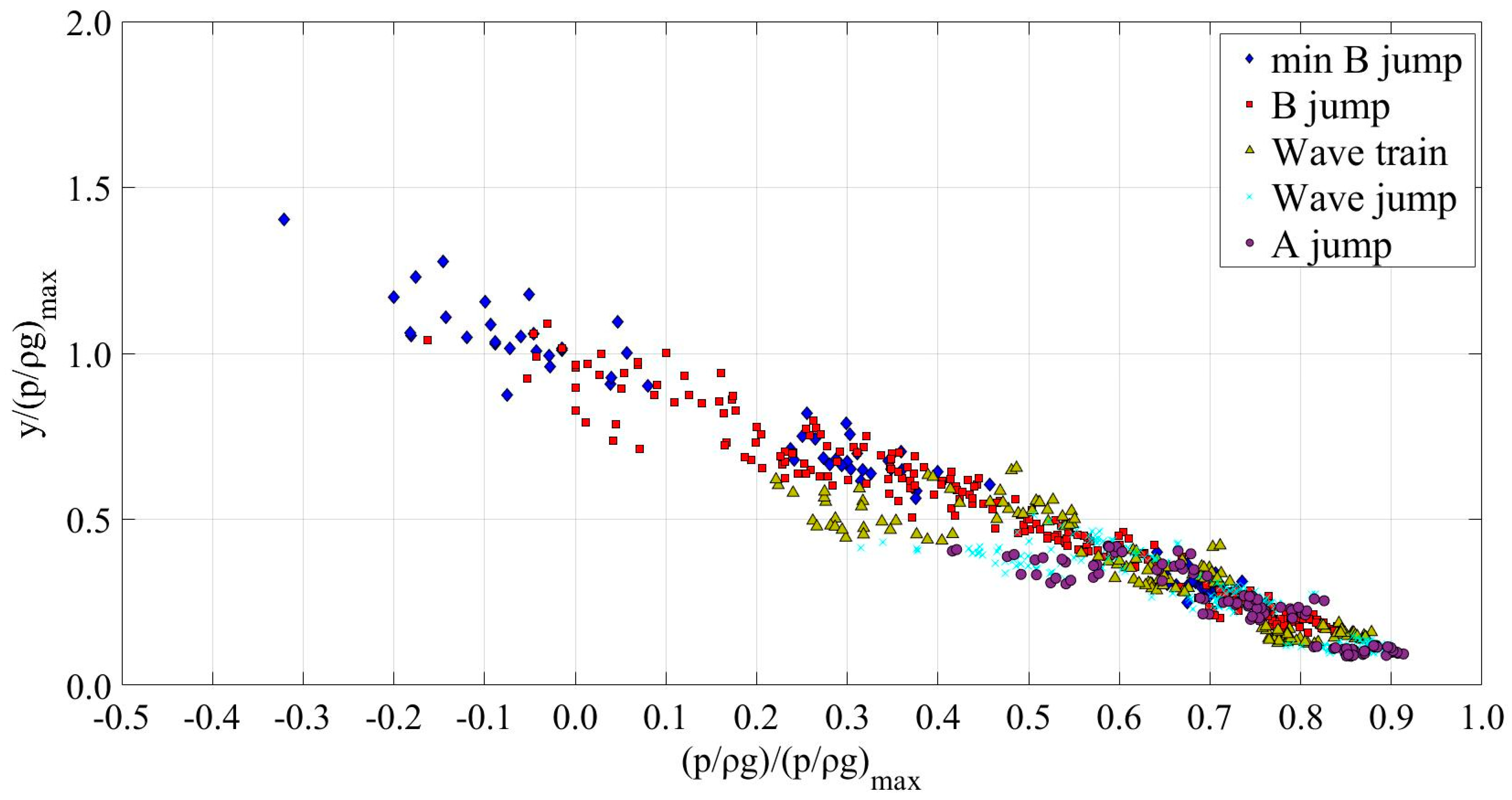
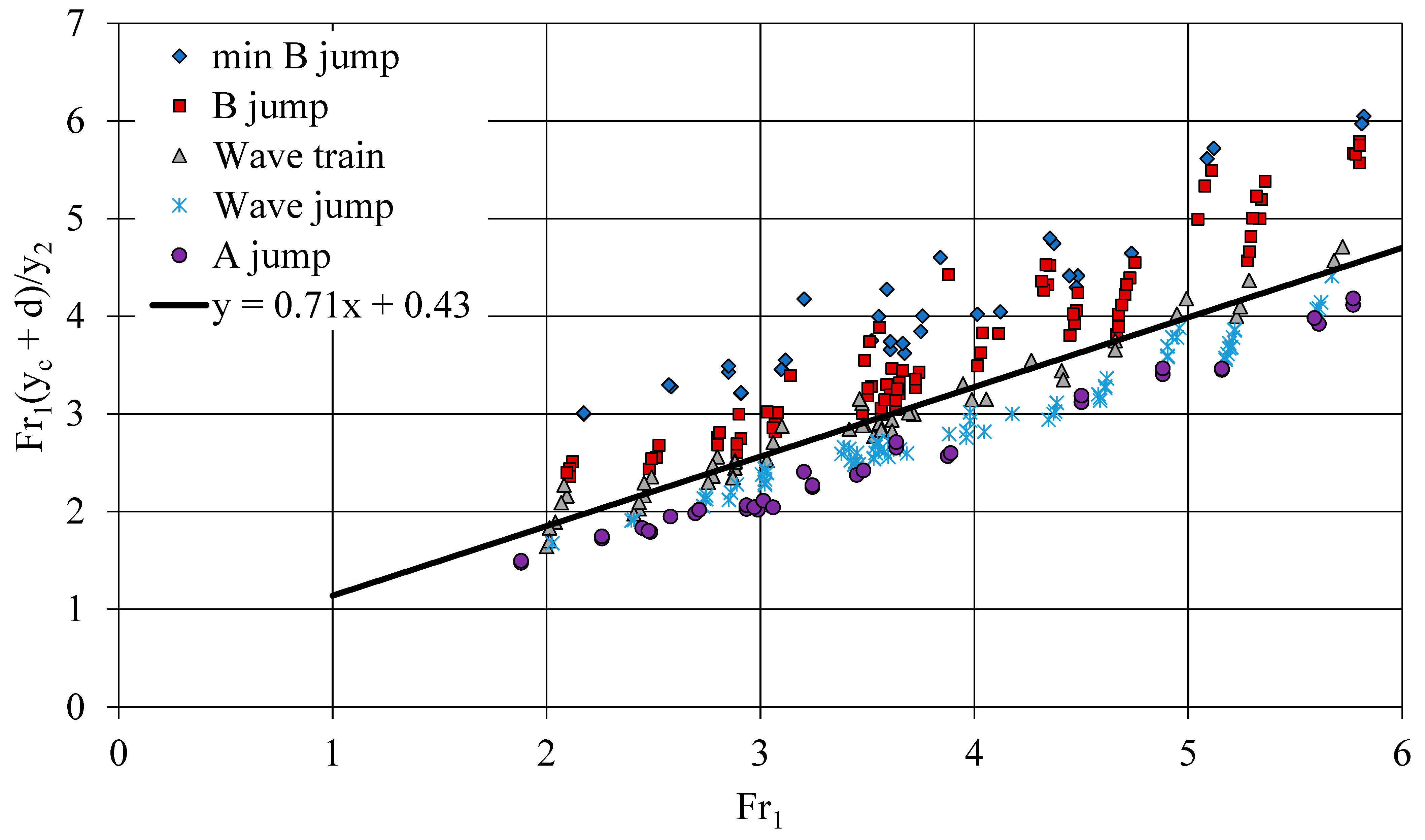
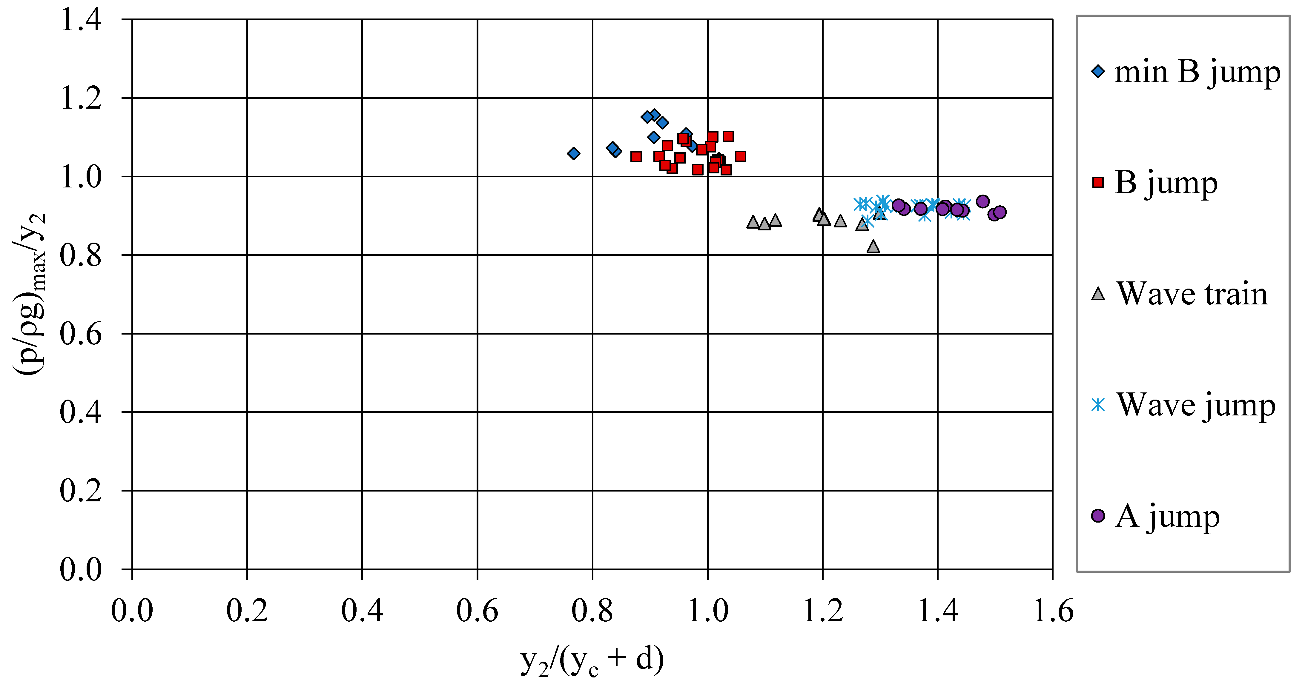
  • Five different types of subcritical flow are observed downstream of a submerged vertical step in an orthogonal channel, minimum B-jump and B-jump where the supercritical jet impinges at the bottom if dimensionless depth y2/(yc + d) < 1.07, and wave-train, wave jump and A-jump when the water jet moves at the surface if y2/(yc + d) > 1.07. These can be distinguished if the normalized depth Fr1(yc + d)/y2 is plotted against Fr1.
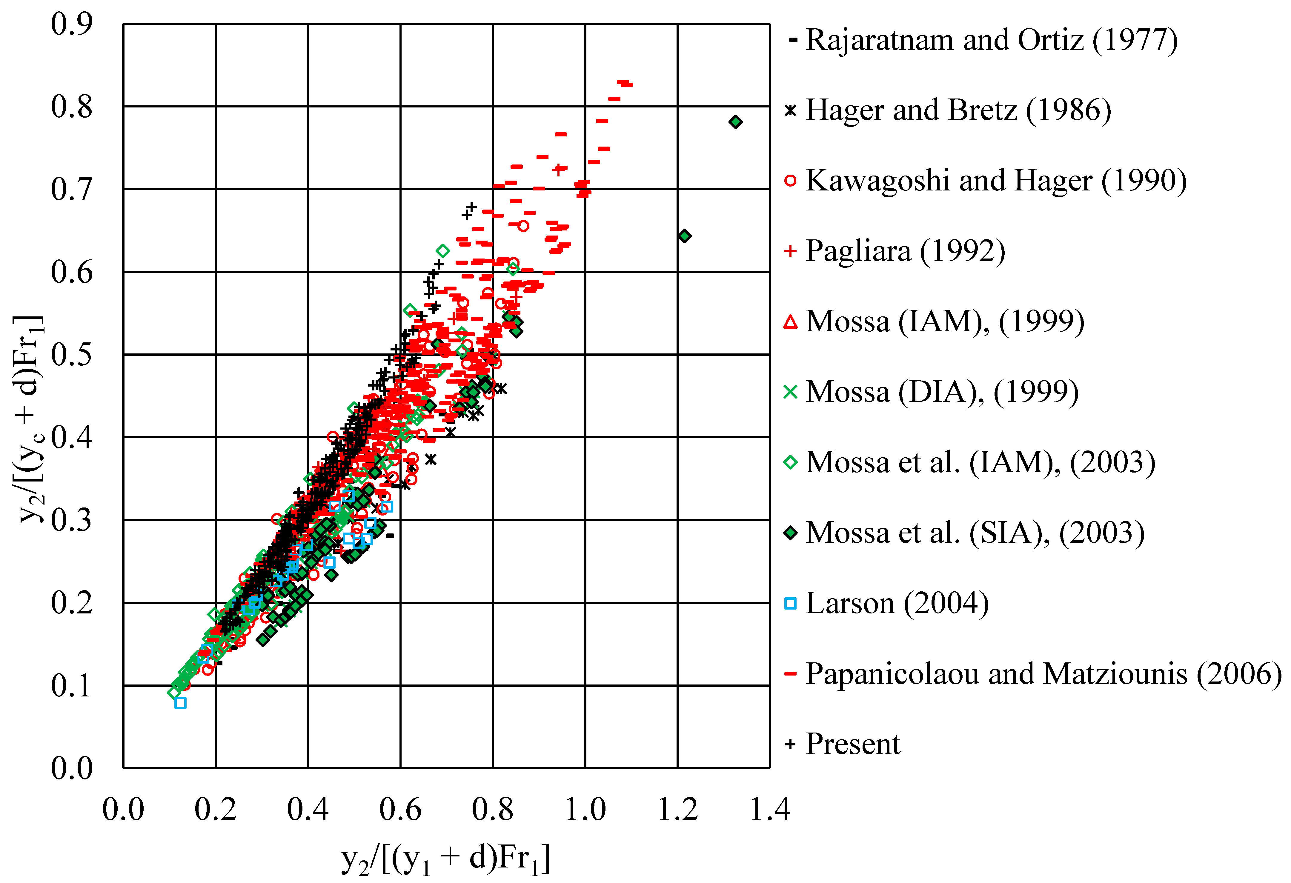
  • For all five different types of flow, there is an equation relating the upstream and downstream depths y1 and y2, the critical depth and Froude number (Figure 5), from which one may compute the step height that fulfills these data.
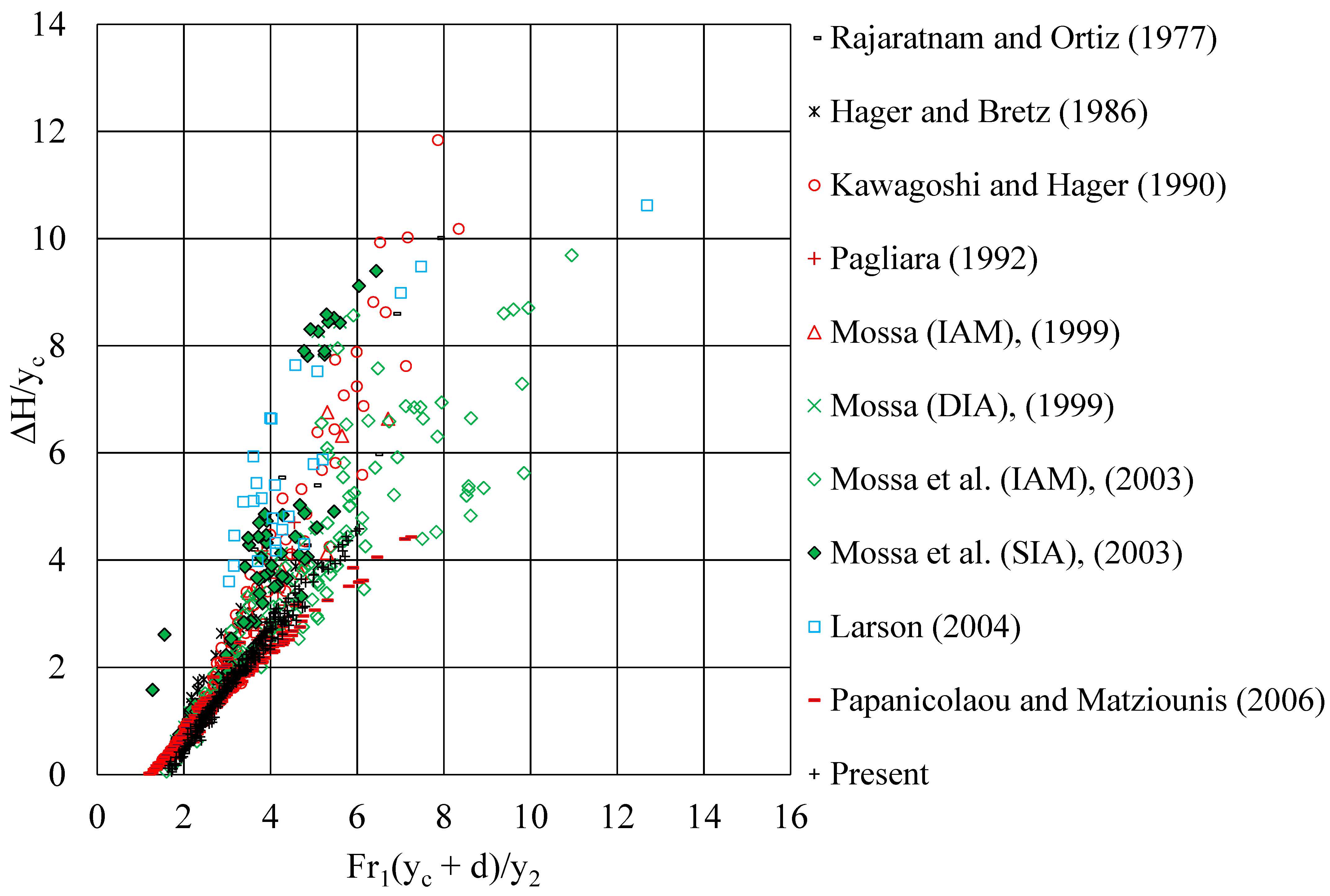
  • The energy loss in dimensionless form ΔH/yc for each type of flow can be estimated using Figure 6, where it is plotted versus the normalized length Fr1(yc + d)/y2.
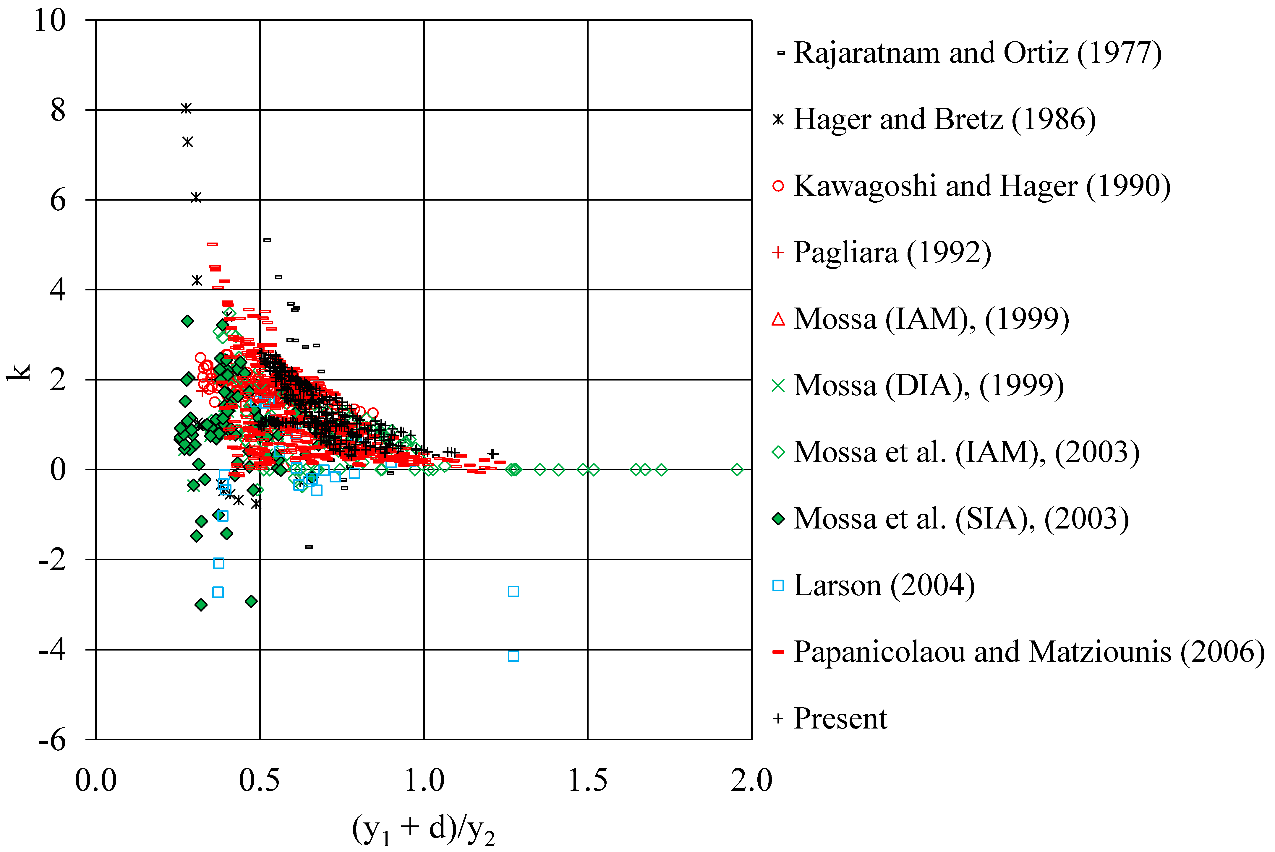
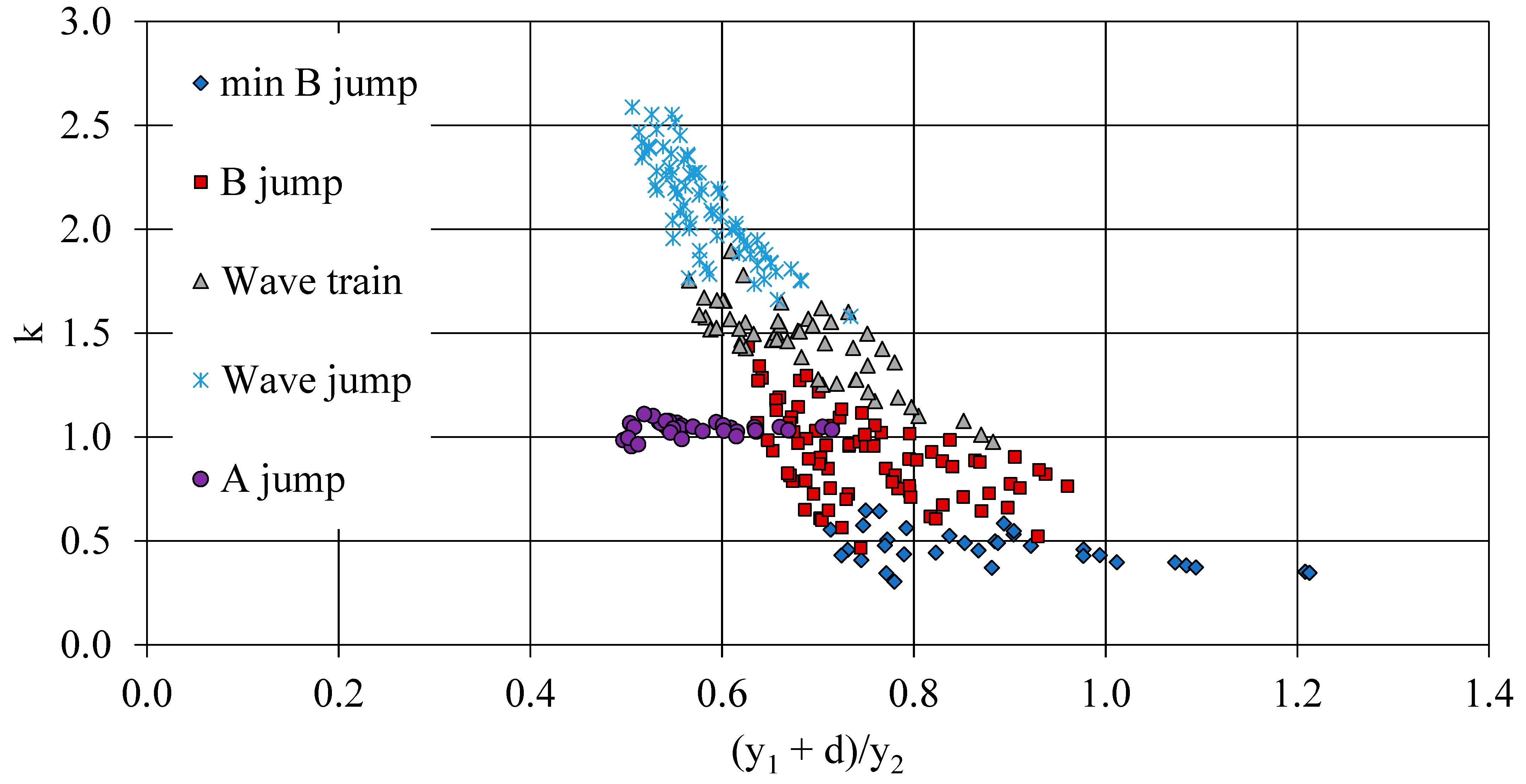
  • Regarding the closure of momentum equation, for the limiting case of minimum B-jump the pressure correction coefficient k = 1/2 is equivalent to pressure force upstream from a linear pressure distribution extended to depth y1 + d but reduced by gd(y1 + d/2)/2 for closure; for the limiting case of A-jump the pressure correction coefficient k = 1 is equivalent to pressure force downstream from hydrostatic pressure distribution to depth (y2 − d) from free the surface for closure.
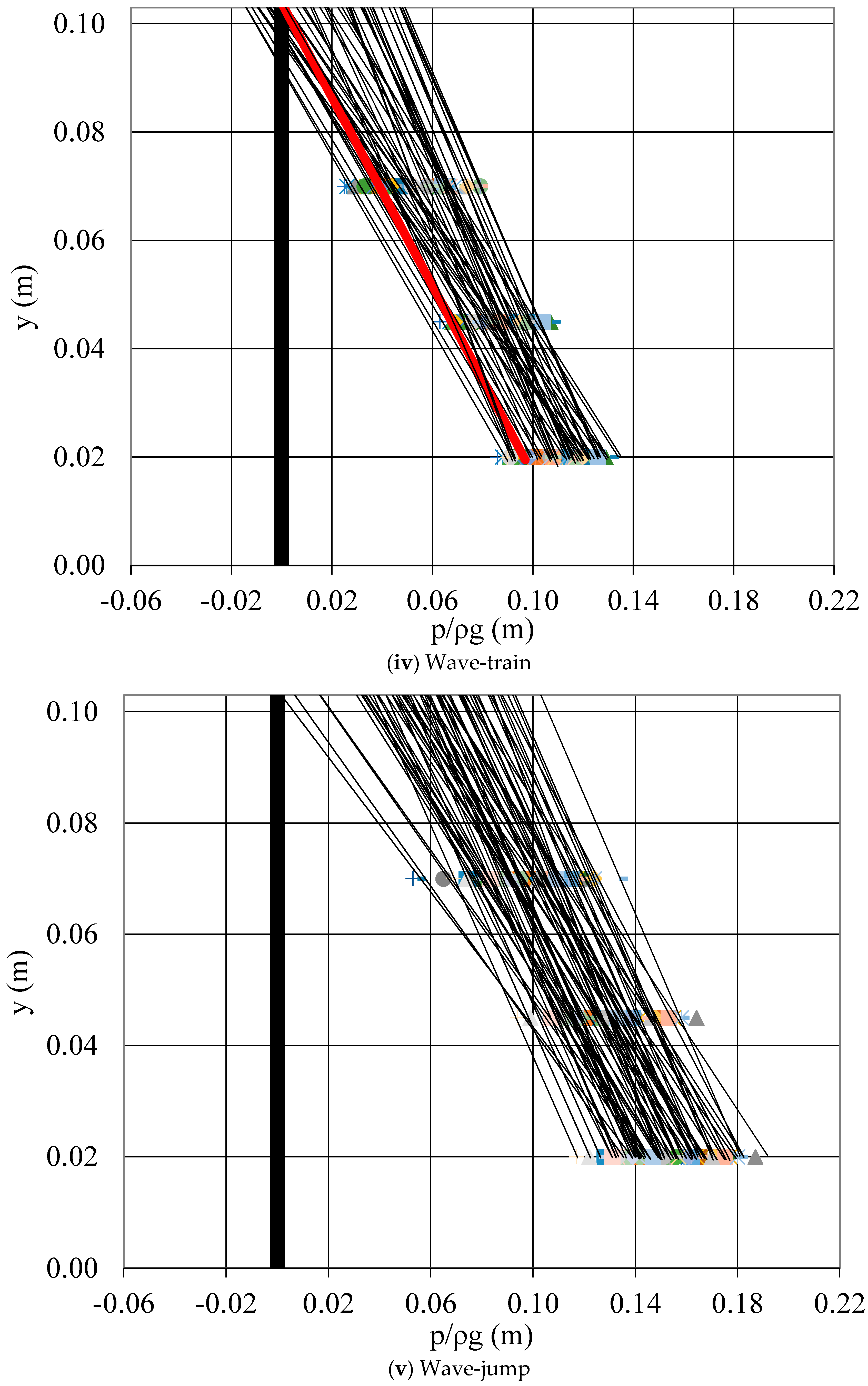
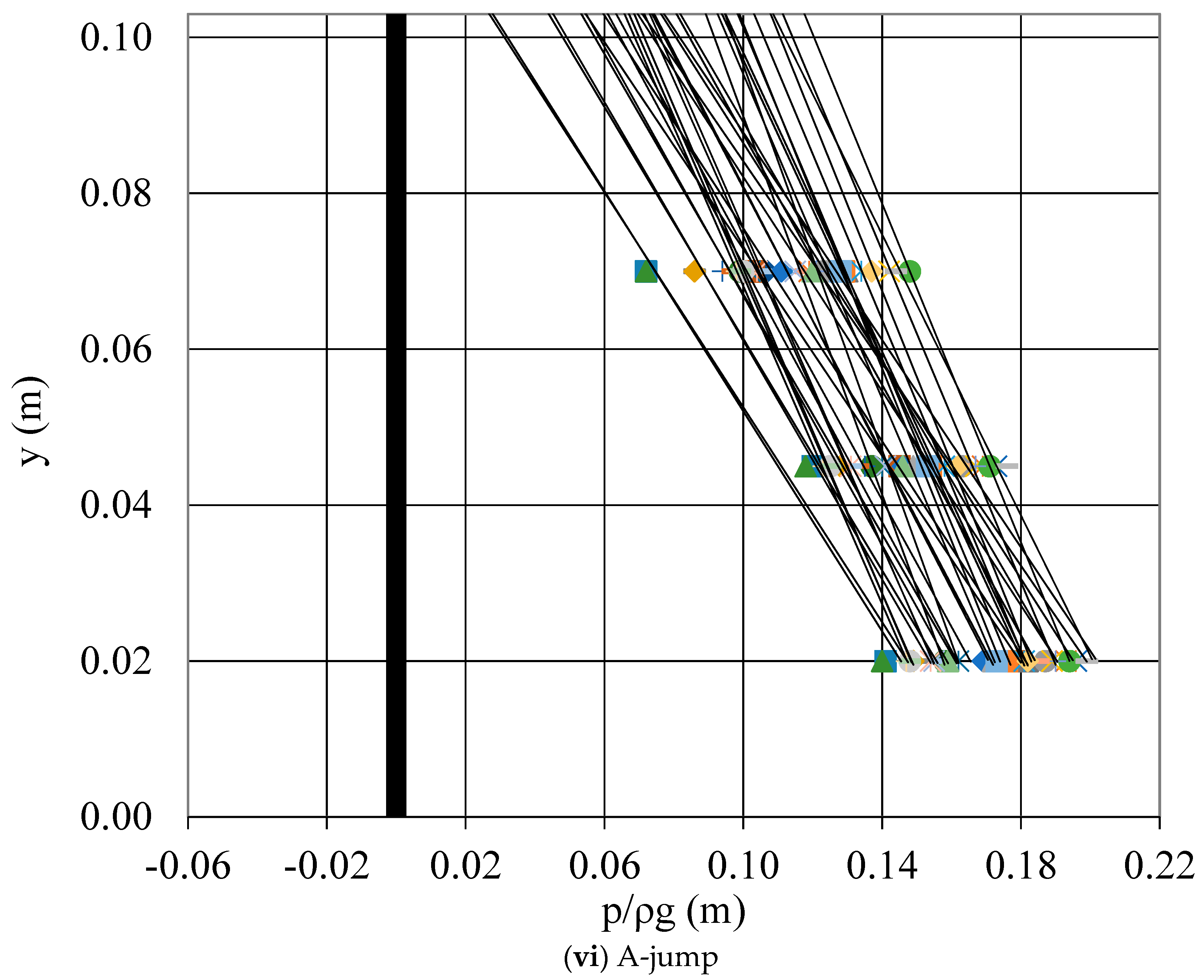
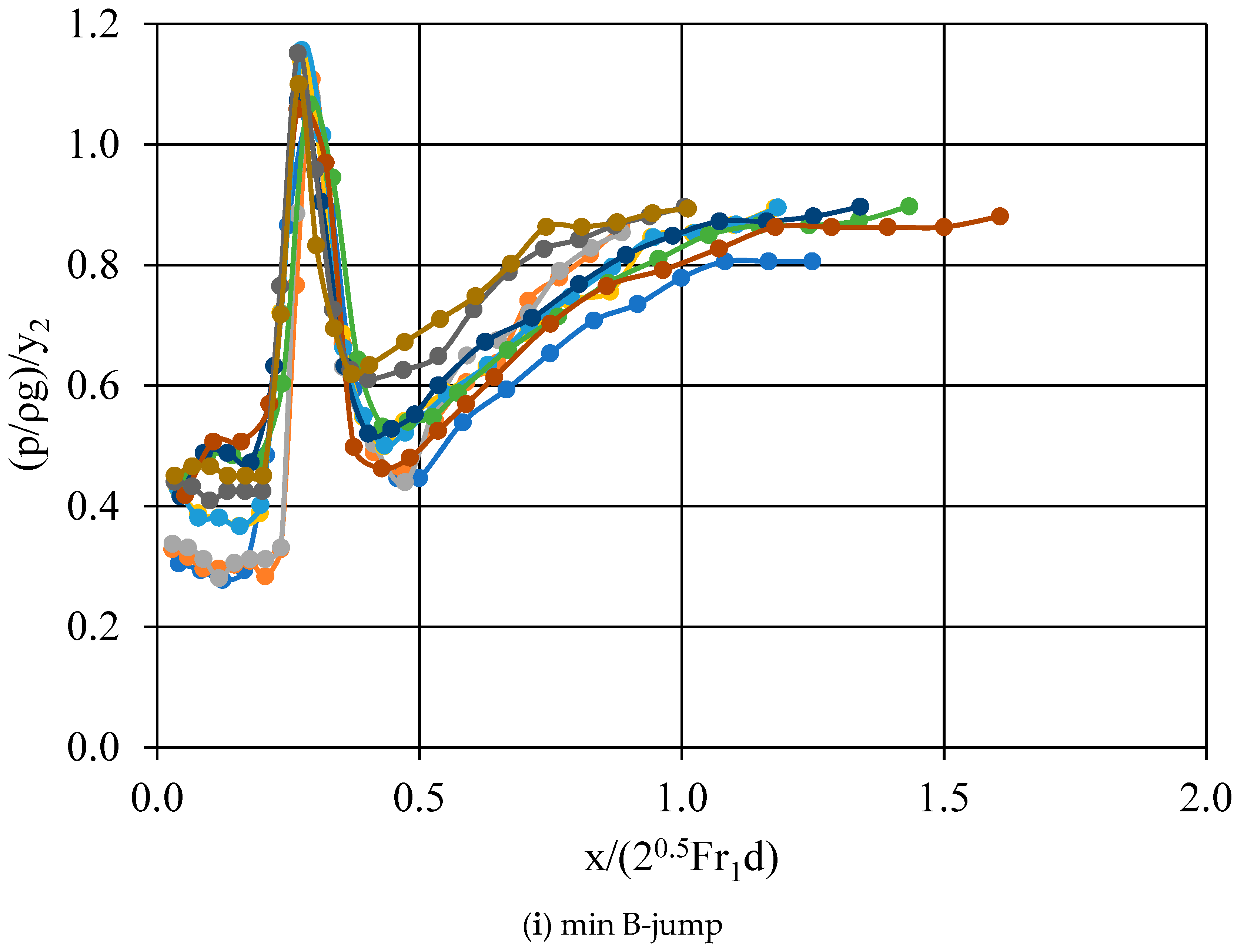
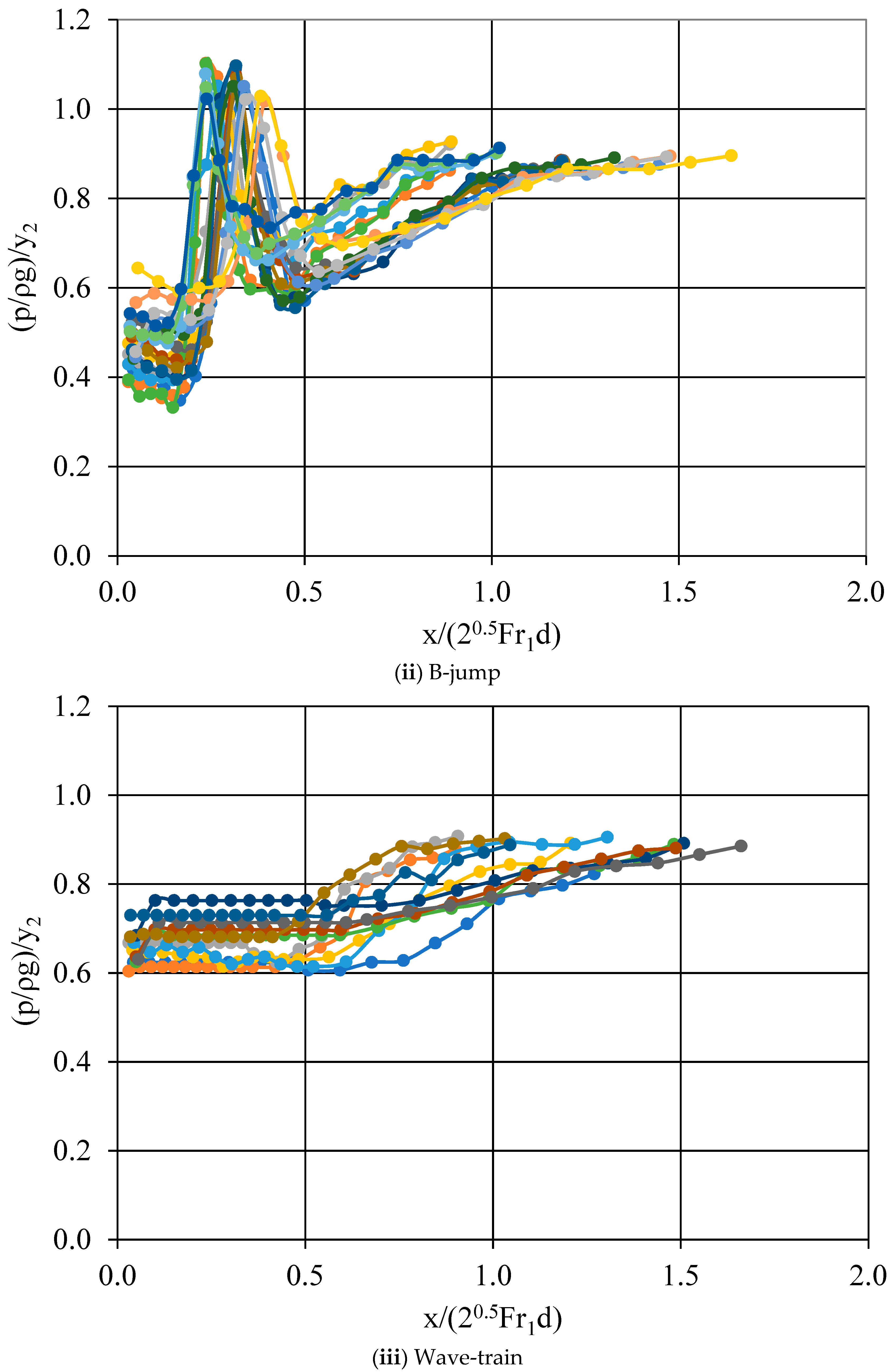
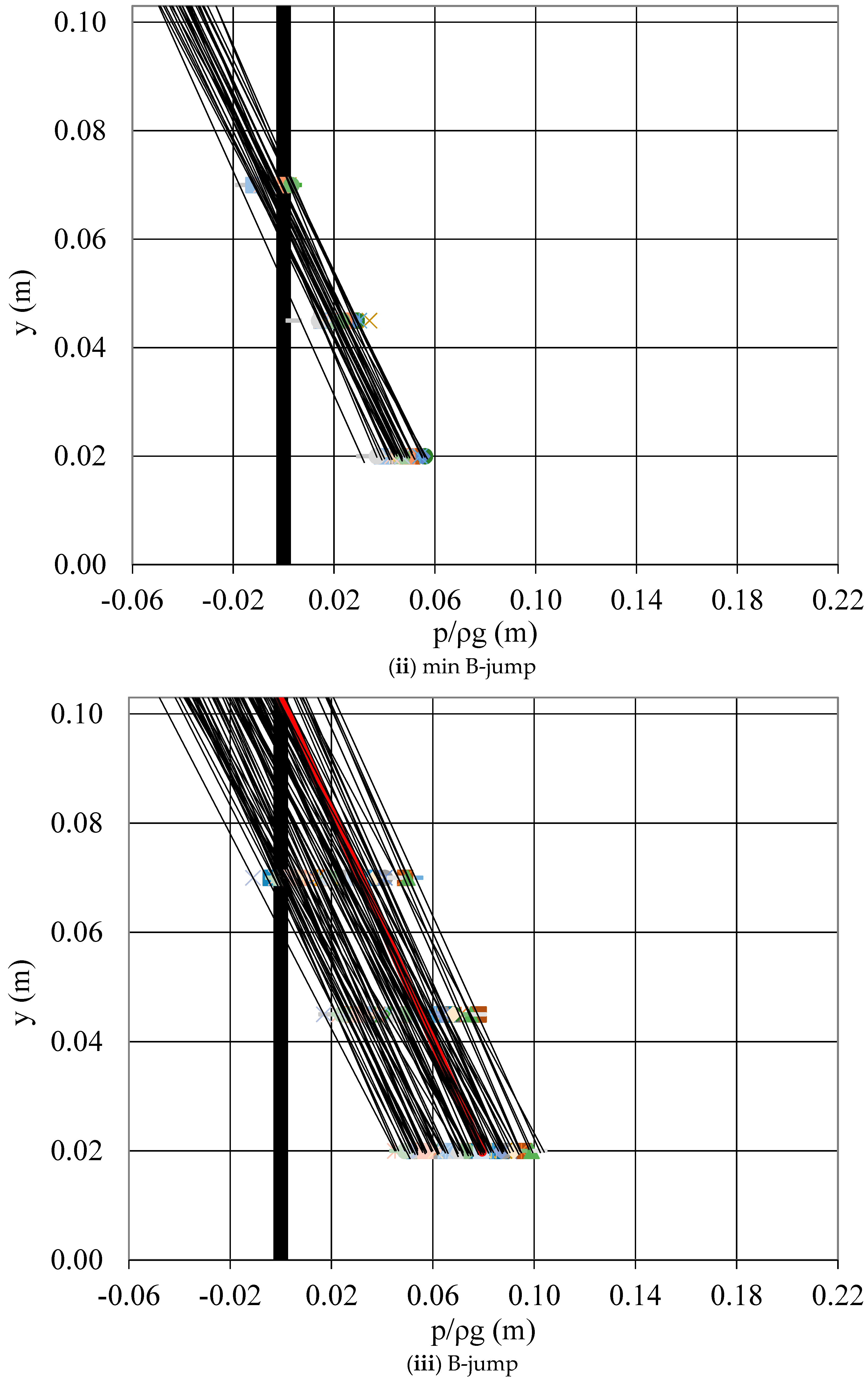
  • The pressure distribution measured at the face of the step was linear. If extended to the top of the step, there was a regime of negative pressure for the minimum B-jump and B-jump types of flow. The pressure head at the bottom downstream of the step showed a maximum that exceeded the tailwater depth for the minimum B-jump and B-jump types of flow, while around the toe was less than y2 for all other types of flow.
  • The present experiment can be useful to the hydraulic engineer in the design of stilling basins with abrupt negative steps and other structures relevant to the dissipation of kinetic energy of water.
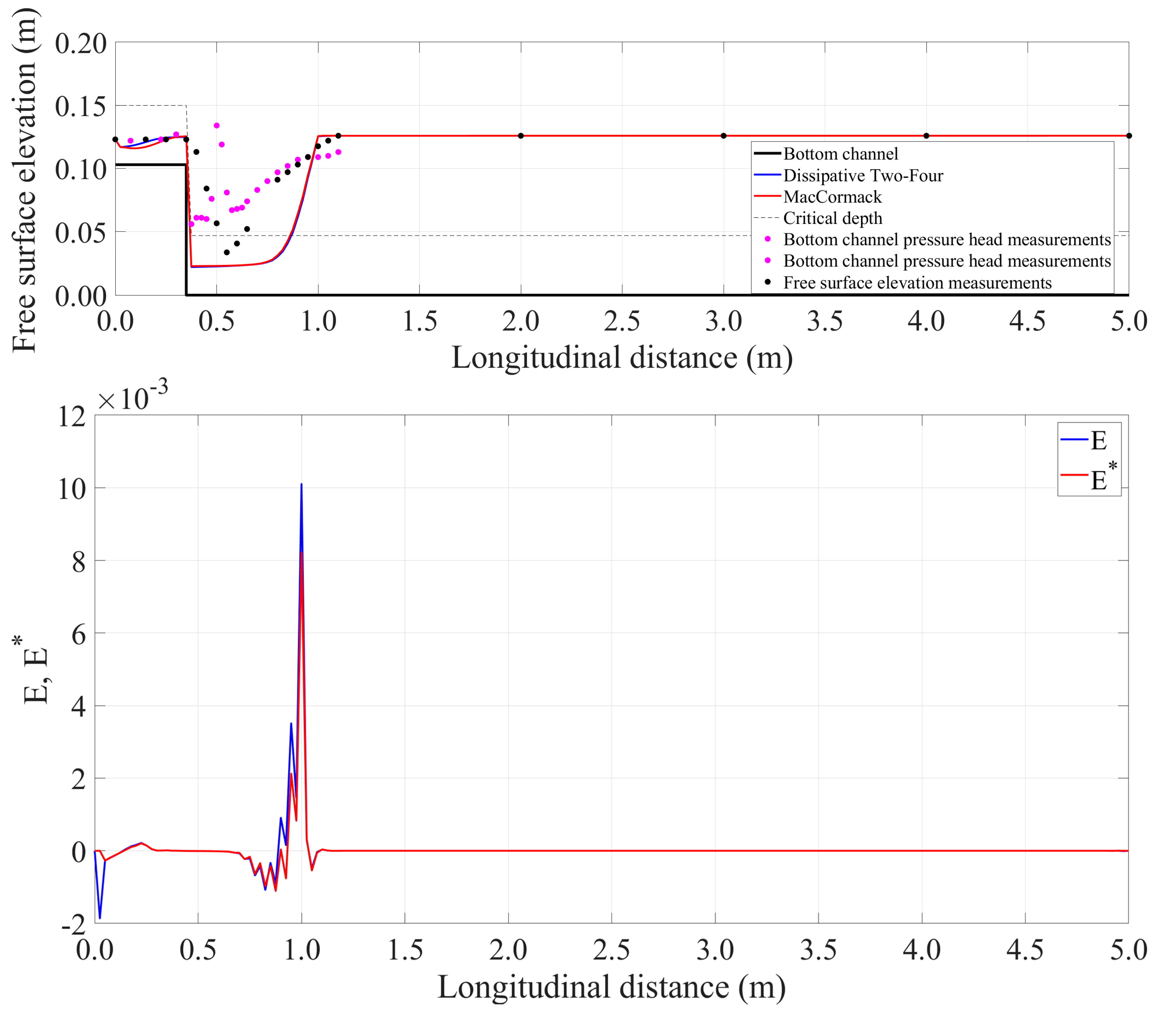
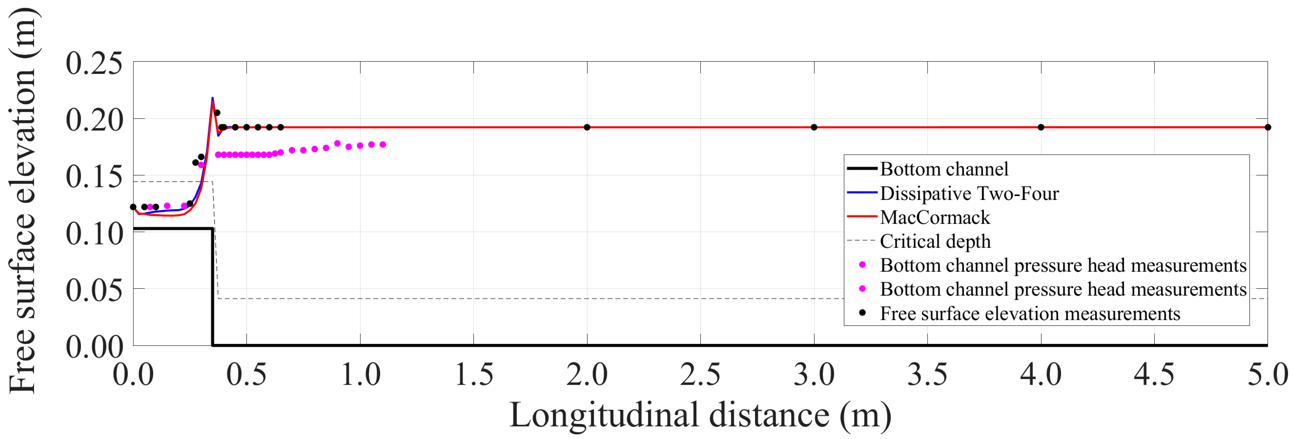
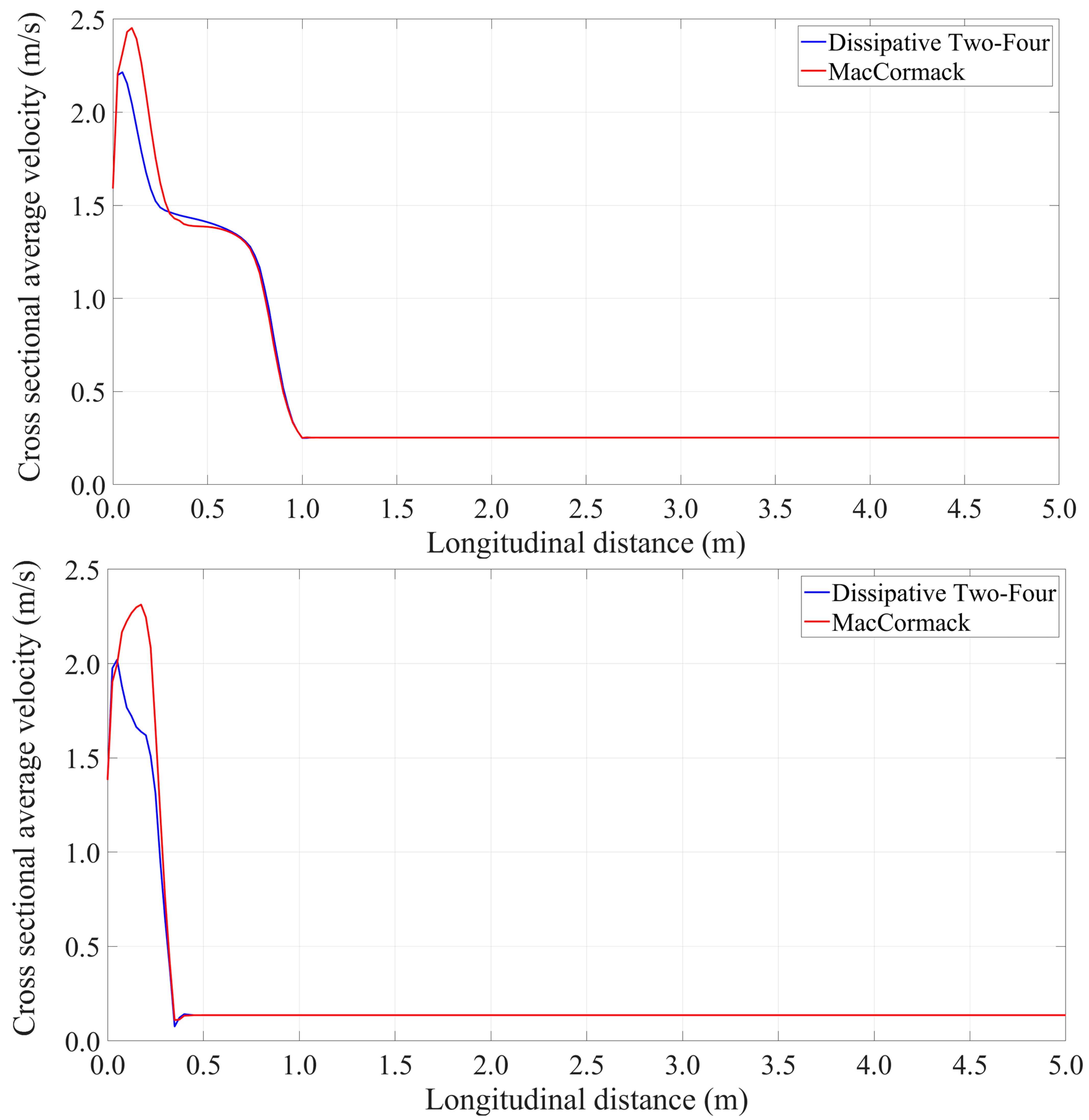
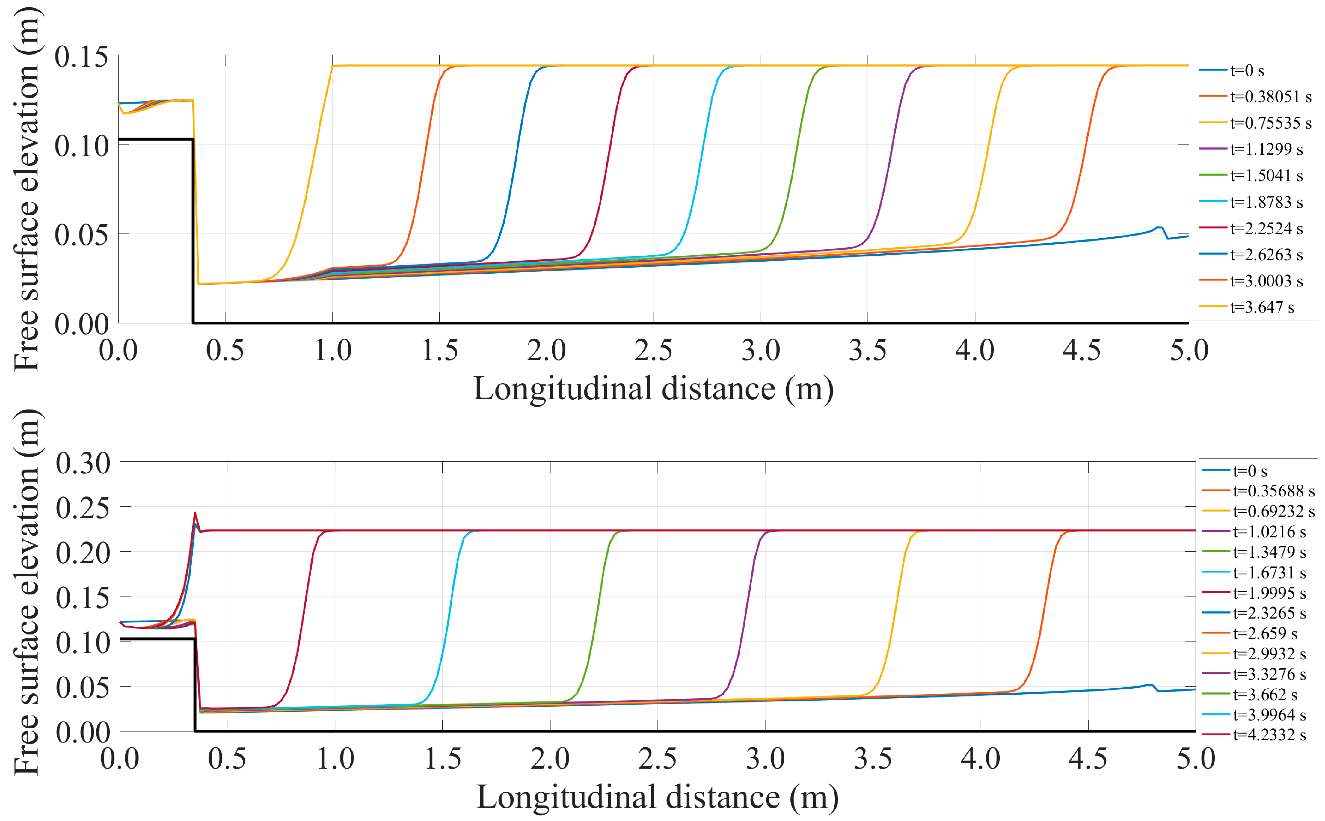
  • The numerical results showed that Boussinesq equations can simulate the basic flow characteristics of the minimum B-jump and the A-jump with acceptable accuracy.

Author Contributions

E.R.: formal analysis and investigation, hardware design, implementation of experiments, code implementation, software, validation, writing—original draft preparation. P.P.: conceptualization, methodology, formal analysis and investigation, supervision, validation, editing—original draft; final approval. All authors have read and agreed to the published version of the manuscript.

Funding

This research received no external funding.

Institutional Review Board Statement

Not applicable.

Informed Consent Statement

Not applicable.

Data Availability Statement

The available datasets analyzed in this study as well as the codes are available upon request from the corresponding author.

Acknowledgments

The financial support by Eugenides Foundation, 387 Sygrou Ave., 17564 Athens, Greece, for the reconstruction of the test section of the channel and construction of the water recirculation system is gratefully acknowledged.

Conflicts of Interest

The authors declare no conflict of interest.

Appendix A

On the Numerical Solution of Boussinesq Equations

The physical and computational grid for the solution of the governing equations is shown in Figure A1. The jump forms inside a horizontal open channel with rectangular cross section of width b and flow rate Q, combining the use of an upstream sluice gate and a downstream sharp crested weir, with the distance between them to be 5.20 m. The longitudinal distance x is measured from the origin set at vena contracta downstream of the sluice gate. The distance between vena contracta and the weir is L = 5.00 m (region where the computational solution is sought) and is discretized by a number of n nodes including the boundary nodes, creating a uniform grid with interval Δx = L/(n − 1). The depth at vena contracta is yup and the depth upstream of the weir where the flow is almost uniform is ydo. The index i denotes the computational grid location, and the upstream and downstream boundaries correspond to nodes i = 1 and i = n with depths yup and ydo respectively. The abrupt drop is located at node i = m and it is treated numerically as a boundary.
Figure A1. Physical and computational domain of the rapidly varied flow in the region of the drop.
Hydrology 09 00074 g0a1
The Boussinesq equations can be solved numerically using two different schemes, the Dissipative Two-Four and the MacCormack scheme. The Dissipative Two-Four scheme consists of a predictor and a corrector step, again for the spatial derivatives of Equation (7), in the predictor step forward finite differences are used and in the corrector step backward finite differences. This scheme includes the spatial nodes i + 2, i + 1 and i in the predictor step (Equation (A1)) and the nodes i, i − 1 and i − 2 in the corrector step (Equation (A2)) respectively, as:
G i * = G i k + λ 6 ( F i + 2 k 8 F i + 1 k + 7 F i k ) + Δ tS i k ,  
G i * * = 1 2 ( G i k + G i * ) + λ 12 ( 7 F i * + 8 F i 1 * F i 2 * ) + 1 2 Δ tS i * ,
The vector G i k + 1 at the next iteration level k + 1 and grid point i is given by:
G i k + 1 = 1 2 ( G i k + G i * * ) ,
where λ = Δt/Δx, Δt being the time step and superscripts k and k + 1 refer to two successive iterations. All variables with asterisk (*) refer to those calculated at the predictor step while all variables with double asterisk (**) refer to those calculated at the corrector step.
The MacCormack scheme is a two-step algorithm scheme. For the spatial derivatives of Equation (7), forward finite differences are used including nodes i + 1 and i in the predictor step (Equation (A4)), while in the corrector step backward finite differences are used including the nodes i and i − 1 (Equation (A5)) as:
G i * = G i k λ ( F i + 1 k F i k ) + Δ tS i k ,
and
G i * * = G i * λ ( F i * F i 1 * ) + Δ tS i * .
The flow variables at the next iteration level k + 1 and grid point i are given by Equation (A3).
Denoting i to be the spatial node and k the iteration number, the second order derivative in the Boussinesq term 2 u / x 2 is approximated by a three point central finite difference in both steps, predictor and corrector. Forward finite difference is used in the predictor step (Equation (A6)) and backward finite difference in the corrector step (Equation (A7)) for the first order derivative u / x   as:
E i = u i k u i + 1 k 2 u i k + u i 1 k Δ x 2 ( u i + 1 k u i k Δ x ) 2 ,  
E i * = u i * u i + 1 * 2 u i * + u i 1 * Δ x 2 ( u i * u i 1 * Δ x ) 2 .
The mixed partial derivative 2 u / x t has been ignored since it is zero at steady state.
The appropriate initial and boundary conditions must be set in order to have a well posed problem [27]. At time t = 0 two characteristic curves enter at the computational domain, so the flow depth and the streamwise velocity must be specified at each grid point. An auxiliary condition has to be specified for each characteristic curve entering the boundaries of the computational domain, which includes the steady, gradually varied supercritical flow, in the entire length of the channel. From the steady gradually varied flow equation:
dy dx = S o S f 1 Fr 2
the flow depth and velocity are computed at each grid point numerically using the Kutta-Merson method with known initial depth upstream, so the calculations can proceed downstream at each grid point. The initial depth yup is that at the exit of the sluice gate, while Fr = u / gy   is the Froude number of the flow.
The flow conditions at each boundary are fixed. At node i = 1 (Figure A1) the flow is supercritical with depth yup while at node i = n the flow is subcritical with depth ydo. During the iteration process the flow depths at nodes i = 1, i = n, are constant and known from the experimental measurements taken downstream of the sluice gate and upstream of the weir, respectively. The velocity at i = 1, uup, is also constant and known, uup = Q/byup, while at i = n it has to be computed.
The velocity at the downstream boundary node i = n will be estimated with the method of specified intervals and the positive characteristic equation discretized by finite differences. In Figure A1 points A and B correspond to the nodes n − 1 and n respectively, at time level k, while the positive characteristic passing through the point P with the unknown velocity at the downstream boundary at the time level k + 1 is indicated. The point R is the intersection of the positive characteristic passing through the point P with the grid line of the time level k. With the method of specified intervals the velocity, the celerity and the flow depth at point R respectively, are calculated [32] from Equations (A9)–(A11) as
u R = u B + λ ( c B u A c A u B ) 1 + λ ( u B u A + c B c A ) ,
c R = c B + λ u R ( c B c A ) 1 + λ ( c B c A ) ,  
y R = c R 2 / g ,  
where c = gy is the celerity of the propagating wave inside a rectangular open channel of small amplitude in shallow water and u A = u n 1 k , u B = u n k , c A = gy n 1 k and c B = gy n k . The energy line slope at point R is estimated as:
S f R = n f 2 u R 2 / R R 4 / 3 ,
where RR = byR/(b + 2yR). Then the velocity at point P i.e., the variable u n k + 1 at iteration k + 1, can be computed from the following relationship:
u P = u n k + 1 = u R + 2 c R 2 gy n k + 1 g Δ t ( S f R S o ) ,
The unknown flow variables at the step were computed using the method of specified intervals. In the case of the minimum B jump the flow is supercritical at the step. The depth and the velocity at node, i = m will be calculated using the positive and the negative characteristic curves. In Figure A2a, points A and B correspond to nodes m − 1 and m respectively, at time level k, while the positive and negative characteristics passing through point P with the unknown flow depth and velocity at node m at the time level k + 1 are indicated. The point R is the intersection of the positive characteristic through point P with the grid line of time level k. The method of specified intervals computes the velocity, the celerity, the flow depth and the energy line slope at point R with Equations (A9)–(A12). The point S is the intersection of the negative characteristic passing through point P with the grid line of time level k. The velocity, the celerity, the flow depth and the energy line slope at point S through the negative characteristic curve are computed [32] from Equations (A14)–(A17) as
u S = u B λ ( c B u A c A u B ) 1 + λ ( u B u A c B + c A ) ,
c S = c B λ u S ( c B c A ) 1 λ ( c B c A ) ,
y S = c S 2 / g ,
S f S = n f 2 u S 2 / R S 4 / 3 ,
In Equations (A9), (A10), (A14) and (A15), it is u A = u m 1 k , u B = u m k , c A = gy m 1 k , c B = gy m k and RS = byS/(b + 2yS). Then, the flow depth and the velocity at point P i.e., the variables y m k + 1 , u m k + 1 , at iteration k + 1 can be computed from the following equations:
y P = y m k + 1 = { 0.25 [ u R u S + 2 ( c R + c S ) g Δ t ( S f R S f S ) ] } 2 / g ,
u P = u m k + 1 = 0.5 [ u R + u S + 2 ( c R c S ) g Δ t ( S f R + S f S ) ] ,
Figure A2. Characteristic curves at the drop: (a) Supercritical flow; (b) Subcritical flow.
Hydrology 09 00074 g0a2
In the case of the A-jump the flow is subcritical at the step. The difference in comparison with the minimum B-jump is the direction of the negative characteristic curve shown in Figure A2b. In Figure A2b, points A, B and C correspond to nodes m − 1, m and m + 1 respectively at time level k, while the positive and the negative characteristics passing through point P with unknown flow depth and velocity at node m at the time level k + 1 are indicated. The point R is the intersection of the positive characteristic passing through point P with the grid line of time level k. The velocity, the celerity the flow depth as well as the energy line slope at point R are calculated from Equations (A9)–(A12) with u A = u m 1 k , u B = u m k . Point S is the intersection of the negative characteristic passing through point P with the grid line of time level k. The velocity, the celerity, the flow depth as well as the energy line slope at point S through the negative characteristic curve are computed [32] from Equations (A20)–(A23) as
u S = u B + λ ( c B u C c C u B ) 1 + λ ( u C u B c B + c C ) ,  
c S = c B + λ u S ( c B c C ) 1 + λ ( c B c C ) ,
y S = c S 2 / g ,  
S f S = n f 2 u S 2 / R S 4 / 3 ,
where u B = u m k , u C = u m + 1 k , c B = gy m k , c C = gy m + 1 k and RS = byS/(b + 2yS). Then the flow depth and velocity at point P i.e., the variables y m k + 1 , u m k + 1 at iteration k + 1 can be computed from Equations (A18) and (A19), respectively.
The time step Δt, was variable in each iteration satisfying the Courant-Friedrichs-Lewy condition for all spatial nodes for stability reasons, calculated from the following relationship:
Δ t = c n Δ x max ( | u i k | + gy i k ) ,  
where cn is the Courant number which must be less than or equal to 0.65 [28] and Δx is the constant spatial step as shown in Figure A1.
High oscillations occur in the region of the jump; therefore, in order to filter them out, artificial viscosity had to be added to the numerical schemes. According to Chaudhry [27] we implement the following. First the parameter ξi at computational node i and at iteration k + 1 is calculated as:
ξ i k + 1 = | y i + 1 k + 1 2 y i k + 1 + y i 1 k + 1 | | y i + 1 k + 1 | + 2 | y i k + 1 | + | y i 1 k + 1 | ,   for   the   interior   nodes
ξ i k + 1 = | y i + 1 k + 1 y i k + 1 | | y i + 1 k + 1 | + | y i k + 1 | ,   for   the   upstream   end   node
ξ i k + 1 = | y i k + 1 y i 1 k + 1 | | y i k + 1 | + | y i 1 k + 1 | ,   for   the   downstream   end   node
Then at the center of the segment between node i and node i + 1 it is:
ξ i + ( 1 / 2 ) k + 1 = k art Δ x Δ t max ( ξ i k + 1 , ξ i + 1 k + 1 ) ,
Similarly between node i − 1 and node i
ξ i ( 1 / 2 ) k + 1 = k art Δ x Δ t max ( ξ i 1 k + 1 , ξ i k + 1 ) ,
where kart is the coefficient adjusting the amount of dissipation. Finally the flow depth and the velocity are modified to the new ones according to the following equation:
f new i k + 1 = f old i k + 1 + ξ i + ( 1 / 2 ) k + 1 ( f old i + 1 k + 1 f old i k + 1 ) ξ i ( 1 / 2 ) k + 1 ( f old i k + 1 f old i 1 k + 1 ) ,
where f is either the flow depth or the velocity.
The developed algorithm for each numerical scheme consists of the following steps:
  • Compute the flow depth and velocity at all computational spatial nodes at initial time (t = 0) according to the initial condition of the problem.
    At first iteration:
  • Set up the depths yup and ydo at the upstream and downstream boundary nodes respectively, known from the experimental measurements.
  • Compute the vector G i * in the predictor step, the vector G i ** in the corrector step and the vector Gi for all internal computational spatial nodes except for the node where the drop is placed.
  • Compute the vector Gi at the location of the drop and the velocity at the downstream boundary node with the specified intervals method.
  • Compute ξi and ξi±(1/2) and modify the flow depth and velocity according to Equation (A30).
  • Repeat steps 2–5, with the computed depth and velocity of the present iteration to be the starting values for the next iteration. The algorithm iterates until the change of the depth between two successive iterations in all computational spatial nodes is less than a fixed convergence value. Then the minimum B-jump or the A-jump form as part of the steady state solution.

References

  1. Gualtieri, C.; Chanson, H. Physical and Numerical Modelling of Air-Water Flows: An Introductory Review. Environ. Model. Softw. 2021, 143, 105109. [Google Scholar] [CrossRef]
  2. Moore, W.L.; Morgan, C.W. The Hydraulic Jump at an Abrupt Drop. J. Hydraul. Div. Proc. Am. Soc. Civ. Eng. 1957, 83, 1–21. [Google Scholar] [CrossRef]
  3. Ohtsu, I.; Yasuda, Y. Transition from Supercritical to Subcritical Flow at an Abrupt Drop. J. Hydraul. Res. 1991, 29, 309–328. [Google Scholar] [CrossRef]
  4. Mossa, M.; Petrillo, A.; Chanson, H. Tailwater Level Effects on Flow Conditions at an Abrupt Drop. J. Hydraul. Res. 2003, 41, 39–51. [Google Scholar] [CrossRef] [Green Version]
  5. Hager, W.H. B-Jumps at Abrupt Channel Drops. J. Hydraul. Eng. 1985, 11, 861–866. [Google Scholar] [CrossRef]
  6. Hager, W.H.; Bretz, N.V. Hydraulic Jumps at Positive and Negative Steps. J. Hydraul. Res. 1986, 24, 237–253. [Google Scholar] [CrossRef]
  7. Pagliara, S. Wave Type Flow at Abrupt Drop: Flow Geometry and Energy Loss, Entropy and Energy Dissipation in Water Resources. In Water Science and Technology Library; Kluwer Academic Publishers: Drive Norwell, MA, USA, 1992; Volume 9, pp. 469–479. [Google Scholar]
  8. Ohtsu, I.; Yasuda, Y. Discussion of Hydraulic Jumps at Positive and Negative Steps by Hager and Bretz. J. Hydraul. Res. 1987, 25, 407–413. [Google Scholar] [CrossRef]
  9. Pagliara, S. Discussion of Transition from Supercritical to Subcritical Flow at an Abrupt Drop by Ohtsu and Yasuda. J. Hydraul. Res. 1992, 30, 428–432. [Google Scholar] [CrossRef]
  10. Negm, M.A. Analysis of Pressure Distribution Coefficient on Steps Under Hydraulic Jump Conditions in Sloping Stilling Basins. Trans. Ecol. Environ. 1998, 19, 1–10. [Google Scholar]
  11. Giudice, D.G.; Gisonni, C.; Rasulo, G. Vortex Drop Shaft for Supercritical Flow. In Proceedings of the 16th IAHR-APD Congress and 3rd Symposium of IAHR-ISHS, Nanjing, China, 20–23 October 2008. [Google Scholar]
  12. Rajaratnam, N.; Ortiz, N. Hydraulic Jumps and Waves at Abrupt Drops. J. Hydraul. Div. Proc. Am. Soc. Civ. Eng. 1977, 103, 381–394. [Google Scholar] [CrossRef]
  13. Mossa, M. On the Oscillating Characteristics of Hydraulic Jumps. J. Hydraul. Res. 1999, 37, 541–558. [Google Scholar] [CrossRef]
  14. Sunik, S.M. Tailwater Level Effect on Flow Conditions at an Abrupt Drop. In Proceedings of the Nasional Aplikasi Teknologi Prasarana, Wilayah, India, 2 January 2009. [Google Scholar]
  15. Armenio, V.; Toscano, P.; Fiorotto, V. On the Effects of a Negative Step in Pressure Fluctuations at the Bottom of a Hydraulic Jump. J. Hydraul. Res. 2000, 38, 359–368. [Google Scholar] [CrossRef]
  16. Matziounis, P.; Papanicolaou, P. Subcritical and Supercritical Flow Conditions at a Submerged Forward Facing Step. In Proceedings of the 1st International Conference on Experiments/Process/System Modelling/Simulation/Optimization, Athens, Greece, 6–9 July 2005. [Google Scholar]
  17. Esfahani, M.; Bajestan, M. Dynamic Force Measurement of Roughened Bed B-jump at an Abrupt Drop. Arch. Sci. 2012, 65, 47–54. [Google Scholar]
  18. Riazi, R.; Bejestan, M. Analysis Location of Pressure Fluctuation in Hydraulic Jump Over Roughened Bed with Negative Step. Bull. Environ. Pharmacol. Life Sci. 2014, 3, 103–110. [Google Scholar]
  19. Kawagoshi, N.; Hager, W.H. Wave Type Flow at Abrupt Drops. J. Hydraul. Res. 1990, 28, 235–252. [Google Scholar] [CrossRef]
  20. Quraishi, A.; Al-Brahim, A.M. Hydraulic Jump in Sloping Channel with Positive or Negative Step. J. Hydraul. Res. 1992, 30, 769–782. [Google Scholar] [CrossRef]
  21. Ohtsu, I.; Yasuda, Y. Discussion of Hydraulic Jump in Sloping Channel with Positive or Negative Step by Quraishi and Al-Brahim. J. Hydraul. Res. 1993, 31, 712–716. [Google Scholar] [CrossRef]
  22. Larson, E. Energy Dissipation in Culverts by Forcing a Hydraulic Jump at the Outlet. Master’s Thesis, Department of Civil and Environmental Engineering, Washington State University, Pullman, WA, USA, 2004. [Google Scholar]
  23. Papanicolaou, P.; Matziounis, P. Supercritical Flow Conditions Around a Submerged Forward Facing Step. In Proceedings of the 10th National Congress in Management of Water Resources and Protection of Environment, Hellenic Hydrotechnical Association, Xanthi, Greece, 13–16 December 2006. [Google Scholar]
  24. Bakhti, S.; Hazzab, A. Comparative Analysis of the Positive and Negative Steps in a Forced Hydraulic Jump. Jordan J. Civ. Eng. 2010, 4, 197–204. [Google Scholar]
  25. Simsek, O.; Soydan, N.; Gumus, V.; Akoz, M.; Kirkgoz, M. Numerical Modeling of B-Type Hydraulic Jump at an Abrupt Drop. Tek. Dergi 2015, 24, 7215–7240. [Google Scholar]
  26. Padova, D.; Mossa, M.; Sibilla, S. SPH Modelling of Hydraulic Jump Oscillations at an Abrupt Drop. Water 2017, 9, 790. [Google Scholar] [CrossRef] [Green Version]
  27. Chaudhry, H.M. Open-Channel Flow, 2nd ed.; Springer: New York, NY, USA, 2008; pp. 1–528. [Google Scholar]
  28. Gottlieb, D.; Turkel, E. Dissipative Two-Four Methods for Time-Dependent Problems. Math. Comput. 1976, 30, 703–723. [Google Scholar] [CrossRef]
  29. MacCormack, R.W. The Effect of Viscosity in Hypervelocity Impact Cratering. In Proceedings of the AIAA Hypervelocity Impact Conference, Cincinnati, OH, USA, 30 April–2 May 1969. [Google Scholar] [CrossRef]
  30. Valero, D.; Viti, N.; Gualtieri, C. Numerical Simulation of Hydraulic Jumps. Part 1: Experimental Data for Modelling Performance Assessment. Water 2019, 11, 36. [Google Scholar] [CrossRef] [Green Version]
  31. Viti, N.; Valero, D.; Gualtieri, C. Numerical Simulation of Hydraulic Jumps. Part 2: Recent Results and Future Outlook. Water 2019, 11, 28. [Google Scholar] [CrossRef] [Green Version]
  32. Chanson, H. Environmental Hydraulics of Open Channel Flows, 1st ed.; Elsevier: Oxford, UK, 2004; pp. 1–485. [Google Scholar] [CrossRef] [Green Version]
Figure 1. Transition from supercritical to subcritical flow around a vertical step, (i) minimum B-jump, (ii) B-jump, (iii) wave-train, (iv) wave-jump and (v) A-jump.
Hydrology 09 00074 g001
Figure 2. Definition sketch for the momentum and the energy equations.
Hydrology 09 00074 g002
Figure 3. Side view of the open channel.
Hydrology 09 00074 g003
Figure 4. Distinction of the different flow regimes.
Hydrology 09 00074 g004
Figure 5. Relationship between y1, Fr1, d, yc and y2.
Hydrology 09 00074 g005
Figure 6. Normalized energy loss at the step ΔH/yc versus Fr1(yc + d)/y2.
Hydrology 09 00074 g006
Figure 7. Correction coefficient k to balance the momentum equation versus (y1 + d)/y2.
Hydrology 09 00074 g007
Figure 8. Distribution of the measured pressure head at the face of step with three piezometers, extended linearly to the top (i) supercritical flow, (ii) min B-jump, (iii) B-jump, (iv) wave-train, (v) wave-jump, and (vi) A-jump.
Hydrology 09 00074 g008aHydrology 09 00074 g008bHydrology 09 00074 g008cHydrology 09 00074 g008d
Figure 9. Dimensionless pressure head (p/ρg)/(p/ρg)max at the face of the step versus dimensionless vertical distance from bottom y/(p/ρg)max for all types of flow.
Hydrology 09 00074 g009
Figure 10. Distribution of dimensionless measured pressure head along the bottom of the channel versus the dimensionless horizontal distance downstream of the drop (i) min B-jump, (ii) B-jump, (iii) wave-train, (iv) wave-jump, and (v) A-jump.
Hydrology 09 00074 g010aHydrology 09 00074 g010bHydrology 09 00074 g010c
Figure 11. Dimensionless maximum pressure head at the bottom of the channel downstream of the step, versus y2/(yc + d) for all types of jumps.
Hydrology 09 00074 g011
Figure 12. Comparison between the theoretical and the experimental results for the non-dimensionless pressure force at the face of the step for all types of jumps.
Hydrology 09 00074 g012
Figure 13. Test case 1: (Top) Comparison between the computed free surface profile and the experiment (point gauge and pressure head measurements). (Bottom) Numerical results for the Boussinesq term along the channel for the Dissipative Two-Four scheme, prediction and the correction step.
Hydrology 09 00074 g013
Figure 14. Test case 3: (Top) Comparison between the computed free surface profile and the experiment (point gauge and pressure head measurements). (Bottom) Numerical results for the Boussinesq term along the channel length for the MacCormack scheme, prediction and the correction step.
Hydrology 09 00074 g014aHydrology 09 00074 g014b
Figure 15. Numerical results for the mean stream-wise velocity along the channel length: Test case 1 (top), and test case 3 (bottom).
Hydrology 09 00074 g015
Figure 16. Numerical results for the temporal evolution of the jump: Test case 2 (top) for the Dissipative Two-Four scheme, and test case 4 (bottom) for the MacCormack scheme.
Hydrology 09 00074 g016
Figure 17. Comparison of k versus (y1 + d)/y2, from the present and earlier investigations [4,6,7,9,12,13,19,22,23].
Hydrology 09 00074 g017
Figure 18. Comparison of y2/[(yc + d)Fr1] versus y2/[(y1 + d)Fr1], from the present and earlier investigations [4,6,7,9,12,13,19,22,23].
Hydrology 09 00074 g018
Figure 19. Dimensionless energy loss ΔH/yc as a function of Fr1(yc + d)/y2 for all types of jumps [4,6,7,9,12,13,19,22,23].
Hydrology 09 00074 g019
Table 1. Range of initial parameters of supercritical flow upstream of the step.
Q (L/s)q (L/s/m)y1 (cm)y2 (cm)Inflow Fr1Inflow Re
6.46–17.5025.32–68-671.4–3.625.8–26.81.88–5.8223,000–63,000
Table 2. Measured parameters for modeling of the hydraulic jumps.
Test Case/ExperimentQ (L/s)Fryup (m)ydo (m)Type of Jump
18.113.590.02000.1259minimum B
29.884.370.02000.1442minimum B
36.703.200.01900.1922A jump
49.414.500.01900.2234A jump
Table 3. Mass balance error and number of iterations for convergence.
Test Case/ExperimentNumerical SchemeMaximum Mass Conservation Error (%)Iterations
1Dissipative Two-Four
MacCormack
4.01
3.59
6117
5779
2Dissipative Two-Four
MacCormack
4.07
3.64
4866
5067
3Dissipative Two-Four
MacCormack
2.45
2.13
5474
4934
4Dissipative Two-Four
MacCormack
3.92
4.09
5965
6355
Table 4. Main geometric and hydraulic parameters of earlier and the present experiment.
Researchersb (m)d (cm)q (l/s/m)Fr1d/ycFlow Dimensionality
Rajaratnam & Ortiz 1977 [12]0.4103.60–7.6035.79–145.242.97–10.550.40–1.433D
Hager & Bretz 1986 [6]0.5007.6060.00–400.003.93–5.710.36–1.063D
Kawagoshi & Hager 1990 [19]0.5005.00–7.705.98–179.561.99–13.680.37–5.003D
Pagliara 1992 [7,9]0.5003.72–8.459.80–138.001.85–6.900.45–2.783D
Mossa 1999 [13]0.300
0.400
5.30–10.00
3.20–6.52
23.33–62.00
33.93–80.30
3.19–8.87
2.77–9.92
0.72–1.68
0.41–1.06
3D
Mossa et al., 2003 [4]0.300
0.400
5.30–16.00
3.20–6.52
21.47–65.11
33.68–80.37
1.56–10.24
1.78–10.33
0.72–3.58
0.39–1.07
3D
Larson 2004 [22]0.6109.72–30.4895.63–386.224.10–6.410.39–2.223D
Papanicolaou & Matziounis 2006 [23]0.1002.50–10.0029.90–71.501.73–4.910.31–2.173D
Present0.25510.3025.32–67.081.88–5.821.34–2.563D
Publisher’s Note: MDPI stays neutral with regard to jurisdictional claims in published maps and institutional affiliations.

