Article

Flood-Pulse Variability and Climate Change Effects Increase Uncertainty in Fish Yields: Revisiting Narratives of Declining Fish Catches in India’s Ganga River

1
Riverine Ecosystems and Livelihoods Programme, Wildlife Conservation Trust, Mumbai 400001, India
2
Nature Conservation Foundation, Mysore 570017, India
3
School of Environment and Sustainability, Indian Institute for Human Settlements, Bangalore 560080, India
4
Ashoka Trust for Research in Ecology and the Environment (ATREE), Bangalore 560064, India
*
Author to whom correspondence should be addressed.
Hydrology 2022, 9(4), 53; https://doi.org/10.3390/hydrology9040053
Submission received: 20 December 2021 / Revised: 14 March 2022 / Accepted: 22 March 2022 / Published: 25 March 2022
(This article belongs to the Special Issue Aquatic Ecosystems and Water Resources)

Abstract

:
River-floodplains support a significant number of small-scale capture fisheries despite having undergone degradation due to human modification of river flows by dams, pollution, and climate change. River fish production is underpinned by the annual flood-pulse and associated environmental changes that act as cues for spawning and dispersal for most species. However, studies on fish stock declines have focused more on overfishing than on hydroclimatic variability. Therefore, understanding how changes in flood-pulse variability influence fishing effort and yields is critical to inform adaptive fisheries’ management. We investigated hydroclimatic factors driving flood-pulse variability and fish catch–effort dynamics in India’s Ganga River over two decades (2000–2020). We compiled fishers’ narratives of changing fish catches through semi-structured interviews to compare them with our observed trends. Flood amplitude showed increasing variability, longer duration, and earlier rise timings, linked to La Niña and El Niño phases. Catches per unit effort were correlated with total yield and effort but did not decline as fishers thought, despite overall declines in yield over time. Hydroclimatic variability was a more significant driver of changing yields than local fishing pressure. Rising uncertainty in fisheries’ production, in response to increasing flood-pulse variability and altered flows in the Gangetic Plains, may be affecting fishing behaviour and underlying resource conflicts.

1. Introduction

Globally, river floodplains continue to support highly diverse and productive small-scale capture fisheries despite long-term habitat degradation. Wild fish stocks from river floodplains are critical to the livelihood security and nutrition of millions of people, many of whom live on the margins of society [1,2,3]. However, the socioecological system of river-floodplain fisheries has been subject to radical human-induced flow alteration and degradation by dams, barrages, embankments, alterations of sediment fluxes, and pollution [4,5,6,7,8,9]. Many of these changes have created a scarcity of fish resources, leading to conditions that may promote unsustainable fisheries or even conflicts among fishery users. River floodplains are also experiencing effects of climate change as temperatures warm, snowmelt increases, rainfall patterns change, and the frequency of extreme events increases [10,11,12]. However, sustainability discourses have often emphasized declines in fish stocks due to overfishing, rather than tracking responses of fishers to hydroclimatic variability.
Identifying unambiguous responses to change in fishing activity along river systems is complex. River floodplain systems are inherently dynamic, and fishing communities often well-adapted to environmental variability [2,13,14]. Temporary periods of scarcity and abundance (or windfalls) are commonplace, and fishers routinely modify their practices and investments of effort with respect to hydroclimatic variability and pulsing, resulting in “good years” and “bad years” [15,16,17]. However, with increasing uncertainty in environmental conditions caused by anthropogenic impacts, fishers may not be able to respond in the same way. There is growing evidence of nonstationarity and nonlinearity in hydrological and climatic systems (e.g., extreme events, regime shifts [18,19]). Shifting baselines can further aggravate impacts of fishing practices on available fish resources [20,21,22], with serious implications for managing small-scale fisheries [15,23,24].
In particular, these implications manifest in managing resource conflicts between fishery users. Conflicts often result among fishers from standard narratives of “overfishing” and “declining productivity”. However, only a few studies of riverine capture fisheries look at the impacts of fishing pressure and hydrological variability together [25,26]. The reason is obvious: fishery data and trends are messy, especially so in open access river floodplain fisheries. Predictable hydroclimatic changes influencing fisheries’ productivity and abundance dynamics also lead to responses seen in seasonal fishing effort and investments [27,28]. In turn, impacts of fishing on fish population demography and ecology affect responses of fish species to changing environmental factors [29,30,31,32]. Feedbacks between environmental variability and fishing pressure are complex and can also be additive or synergistic. In river systems with active capture fisheries, unravelling the interactions of fishing pressure (effort and practices) and environmental variability [26,33] is therefore critical for a clear understanding of fishery conflicts in relation to typical narratives of declining productivity and lowering catches articulated by those fishing.
For large rivers, flood-pulses play a major role in driving variability in productivity, termed as the “flood-pulse concept” [34]. Flood-pulses can be characterized as waveforms, according to the “River Wave Concept” [35], in terms of the wave’s amplitude (height of wave or difference between maximum and minimum water level in a year), flood-pulse length or wavelength (time duration or distance between crests and troughs), period, and timings and rates of flood rise and fall. In a natural flood-pulse, the river discharge increases by an order of magnitude over the dry-season flow within a matter of one or two months, with similar magnitudes of increase in sediment loads and water temperatures [8,34,35,36,37]. Flood-pulse variability is associated with flow-coupled or decoupled ecological changes in water temperature, exchange of biota, sediments, and nutrients between the river and floodplain leading to regimes of intermittent lateral river connectivity with wetlands and oxbow lakes, in addition to increased flow contributions from upstream reaches [8,34,36,38,39,40,41,42]. The flooding period is often the main breeding season for most tropical and subtropical riverine fishes that depend on water level and temperature cues for fish spawning, migration, and dispersal movements of larvae between river channels and adjacent floodplains [34,36,38,43,44,45,46,47,48]. Fish species physiologically adapt through responses to these changes and can also pre-emptively act to maximize fitness in dynamic and fluctuating environments [49]. Perturbations in hydroclimatic variables thus directly influence fisheries’ productivity [14,28].
In tropical and subtropical river systems, studies have demonstrated that the present state of fishery impacts on fish production is linked to long-term declines in hydroclimatic and ecological conditions (e.g., [50,51,52,53,54,55]). However, long-term data on aggregate fish yields collected through consistent spatial sampling or human effort are either unavailable, or are lacking adequate metadata, or existing government data may not be accessible for use [56,57] from many regions of the developing tropics, with a few notable exceptions (e.g., Mekong, Amazon: [29,55,58,59]). In the Indian subcontinent, these data gaps for river floodplain fisheries have been long lamented [7,57]. The Gangetic Plain is one of the most intensively used river basins in the world and supports millions of artisanal fishers and a great diversity of fishing practices [60]. Yet, it has remained generally wanting in studies on interactions between environmental changes, aggregate fish yields, and fishing effort (but see [31,32,47,61]). The monsoonal flood-pulse is the strongest driver of fish yields and production in the Gangetic Plains [45]. Glacial melt is a smaller but important contributor to river flow in the peak summer [62]. River discharge usually starts increasing from June/July with the arrival of monsoon rainfall. The peak of the flood-pulse from August to late September/early October is followed by a long period of flow recession from November to May, in which a diversity of fishing practices and activity is concentrated [30,45,63,64].
Earlier investigations have found a general declining trend in fish landings, which they attributed mainly to hydrological and climatic change [47,50,54,65,66,67,68,69,70,71]. Reduction in spawn production of IMC from 80% to 30% (out of total spawn collected) between 1961 and 2004 and pollution were noted as major causes of decline [67]. Vass et al. [68] reported a monotonic decline in fish yields at Allahabad on the Ganga River from 1959 to 2004, which they attributed to the construction of dams, pollution, reduction in rainfall, and intensive spawn collection of the commercially valued Indian major carps (see also [54,72]). The decline in the anadromous migrant hilsa fish Tenualosa ilisha upstream of the Farakka barrage constructed in 1975 is also well-documented [67,73].
In this paper, we analyze the interacting effects of hydroclimatic, ecological, and fishing-effort-related drivers on our own data on observed long-term fishery yields and effort in the Ganga River in the Bhagalpur district of Bihar, from 2000 to 2020. We predicted that: (1) in years with strong flood-pulses, yields and catches will both increase due to higher productivity and higher fishing effort, and (2) in years with poor flood-pulses, yields will decline due to lower productivity, and fishing effort will determine catch rates. We test these predictions and discuss the implications of our results for local declines in fish resources and related fishery conflicts and management issues in India’s Gangetic Plains.

2. Materials and Methods
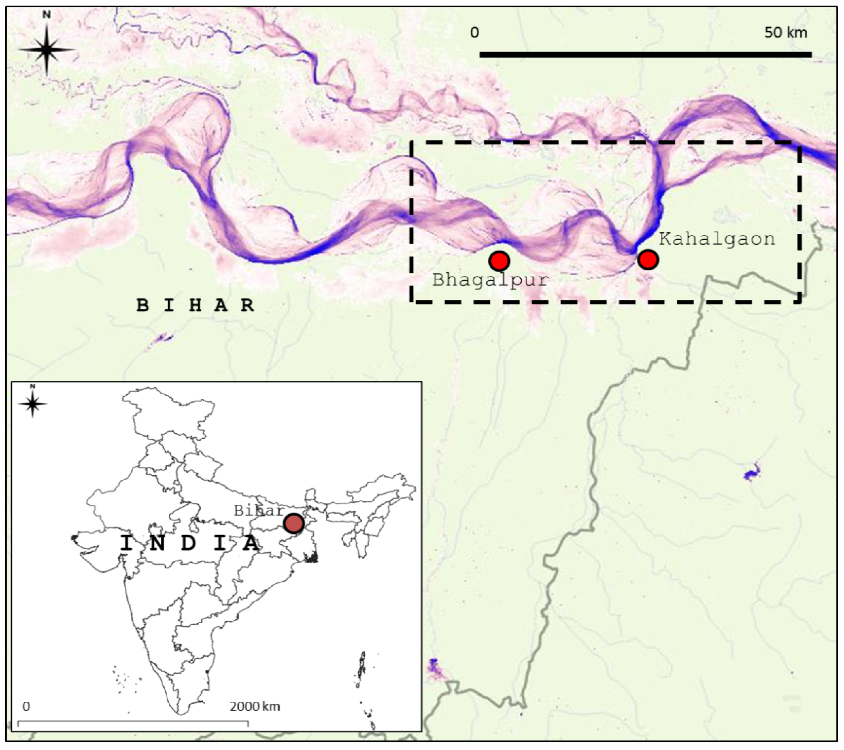
2.1. Study Area

Our study area included two small-scale fisheries, at Bhagalpur and Kahalgaon, on the Ganga River in Bhagalpur district, Bihar, India (Figure 1). This area has active, open access river-based capture fisheries, with about 500 families of almost full-time, resident fishers dependent on the river in 2000. In the last two decades, fishing activity has reduced in terms of the number of total users [74,75,76]. Fishing practices in the area involve the use of gillnets, stake nets, traps, seine nets, and mosquito nets [17,45,77]. Most fishers are landless, live in poverty, and are witnessing severe conflicts over fish resources (details in [17,74,76,78,79,80]), while they also experience resource declines. Mean (30 yr) annual river discharge is 8736 (SD 4845) m3·s−1. Peak flood season discharges range from 16,500 to 50,000 m3·s−1 in September, and the lowest dry-season discharges lie between 2000 and 5000 m3·s−1 in March–April (Figure 2). Spatially, the flood-pulse causes an increase in water spread area by 3 to 12 times, peaking within two months in the region. Mean annual rainfall is around 1200 mm [81]. The river floodplain is characterized by strong monsoon flood-pulses, actively meandering river channels, side channels or chutes, meander cut-offs, oxbow lakes, floodplain wetlands, and palaeo-channels, and high sediment discharge [82,83]. The Farakka barrage on the Ganga River, located approximately 160 km downstream of Bhagalpur, has had significant negative impacts on river hydrology in the region [67,73,84,85,86]. After the Farakka barrage was constructed in 1975, upstream fisheries’ production substantially declined in the study area, with the near collapse of hilsa fisheries [67,73].

2.2. Data Collection

2.2.1. Interviews and Group Discussions with Fishers and Key Informants

Fishers’ perceptions of the reasons for fisheries’ decline were recorded through semi-structured interviews, informal discussions during landing surveys, and focus group discussions with about 100 fishers, key informants, and fish traders at Bhagalpur, Kahalgaon, Naugachhia, and Sultanganj (Bhagalpur district, Bihar). Detailed methods of interview data compilation, compilation, and verification are provided in [17]. We found that fishers typically identified “increased fishing effort” or “overfishing” as a larger driver of the decline in fish resources than environmental change [17]. Fishers may not be in a position to actively link changes in fisheries with hydroclimatic changes. This in turn probably even strengthens their perception of overfishing. To independently investigate this locally dominant perception as a “working hypothesis”, we combined our own monitoring data on fishery yields and aggregate effort, with secondary data on hydroclimatic variables and past data on aggregate fish yields for our study area.

2.2.2. Past Fish Yields and Landings Data

The Central Inland Fisheries Research Institute, Govt. of India, has reported aggregated fish landings and yield data from 1958 to 1997 for Bhagalpur [45,50,66,67]. Based on the taxonomic and temporal resolution of these data, we assessed long-term trends in the percentage of carps, catfishes, and other fish species (of the total yields) after including data from our own monitoring (2000–2020) at Bhagalpur.

2.2.3. Fish Catch–Effort Data from Landing Sites and Market Surveys

We collected monthly, and where possible, daily fish landing site and market survey data from Bhagalpur and Kahalgaon from 2000 to 2020. To our knowledge, this is the longest time-series dataset on fisheries in the Ganga River compiled through informal monitoring by a nongovernmental source in India, despite some gaps and missing years. We used fishery-dependent data on aggregate yields (from market surveys, in kg) and catch-per-unit-effort or CPUE data (from landing site surveys, as the number of fisher days) in the absence of fishery-independent assessments of fish productivity. We typically sampled these sites monthly, spending between 8 and 20 days per month as per the intensity of fishing activity. To standardize aggregated data, we used corrections to indices of total effort for 30 days of each month, accounting for the spatial distribution of effort, and seasonal variations in numbers of fishers and fishing boats [87,88,89,90,91,92,93].
We analyzed daily and monthly variations in fish catch (production) obtained from Bhagalpur (BGP) and Kahalgaon (KHL) on the Ganga River in Bihar. Monthly data on species-wise fish yields were collected from landing sites and fish markets on fish catches, yields, and gear-specific effort at BGP from 2000 to 2020, resulting in 43,055 records for 60 fished species from 2000 to 2020 (with some gaps in 2002, 2009, 2010, 2012, 2014, and 2015 due to logistical issues). At KHL, we compiled available daily fish catch and effort data (n = 47,606 records) from December 2009 to November 2020, from which data on 34 species were analyzed for the 2013–2020 period, which had the fewest data gaps. Fish species were grouped into five categories for analyses: (1) carps (17 species: Cyprinidae), (2) catfish (21 species: Siluriformes), (3) clupeids (5 species of the families Clupeidae and Engraulidae), (4) other fish groups (31 species of other finfish families found in the area), and (5) shrimp (2 species of the Penaeidae and Palaemonidae). We compiled KHL data from market logbooks provided to us by fish traders with their consent, with the conditions of maintaining anonymity and nontransferability of data. The logbooks contained fisher-specific information of daily sold catches, which helped us estimate fishing effort expressed as the number of fisher days per month. We independently corroborated these data from fish landing sites, markets, and boat surveys to ensure the accuracy of recorded information.
The general sampling methods used for landing site and market surveys are also described in [77], which presents an analysis of aggregated fish catch data from Bhagalpur (for 2001–2007) to assess changes in yields and fish composition. However, they [77] did not use data on fishing effort. We ensured that our sampling coverage was similar across seasons in relation to the actual total effort to avoid any systematic seasonal or interannual biases in the aggregated and spatial sampling of catch data [89,91,94,95]. Details of fish species, taxonomy, the annual calendar of fishing, and fish catch/breeding seasonality are in [17].

2.2.4. River Flow Data

River flow data for the Gangetic Plains are “classified” as per Government of India regulations. Therefore, we used an indirect source to obtain discharge estimates. Daily discharge estimates were obtained for the 1998–2020 period from the River Watch 3.5 module of the Flood Observatory, Colorado (www.floodobservatory.colorado.edu, accessed on 31 December 2020; [96]). The estimation of daily discharge in this module is based on a calibration between the microwave reflectance data collected from an AMSR-E satellite-gauging pixel and the predicted flow from a WBMSed model [96]. We used satellite-gauged discharge estimates from the pixel on the Ganga River located at 25.334° N, 86.175° E for this study. Trends in satellite-based discharge estimates were used to assess long-term responses of fish species to the magnitude and variability in river discharge. We validated satellite-gauged estimates for dates (n = 10) with our own direct boat-based field measurements of depth cross-section and channel width data made between 2008 and 2020 using nonlinear regression models. River discharge was estimated from these data using Manning’s equation, which, for large, low-gradient rivers, assumes an equilibrium between flow due to gravity and resistance to flow due to alluvial sediment friction [97,98]. Manning’s equation is as follows: Q = 1 n · A . R 2 3 · S 1 2 , where Q is the estimated river discharge, A is the cross-section area of river channel, Manning’s n is the alluvial roughness coefficient (indicative of frictional forces), R is the hydraulic radius, i.e., cross-section area divided by the wetted perimeter of the river channel, and S the river energy or bed slope, indicative of gravitational force [97,98]. For S, we used the riverbed slope of 6 cm/km provided in a detailed sedimentological and geomorphological study for the same stretch of the Ganga River [82] and incorporated about 15% uncertainty in slope based on downstream and upstream values provided by [82] for calculating flow intervals. To estimate Manning’s n (alluvial roughness coefficient), we used an iterative procedure to calculate the sensitivity of estimated discharge to different n values, which were allowed to vary between 0.03 and 0.04 [99], and the correspondence of predicted discharge estimates within known bounds of river discharge (e.g., from public-accessible data in flood bulletins). From our field measurements, a stage–discharge curve was first estimated for Kahalgaon as Q = 661.43 × e0.0915×S (R2 = 0.81, p < 0.001), where Q is the discharge (m3·s−1) based on Manning’s equation, and S the stage or water level in m recorded in the field. Stage values taken from direct readings of hand-painted gauges on bridge pillars and piers were thus converted into discharge values. We ground-verified the satellite-based discharge (SR) estimates with a regression equation: loge(Q) = 6.48 + 0.25 × loge(SR), (R2 = 0.864, p = 0.0003, F = 44.38, df = 1, 9). This indirect method proved suitable in deriving usable discharge values for our study area and may be promising for use in ungauged large rivers. For additional calibration and confirmation, annual trends in river discharge and water levels were obtained for selected sites (Hathidah, Munger, Bhagalpur, Kahalgaon, Farakka) from published literature [100] and satellite-altimetry-based water level estimates (at 35 day intervals) for points close to these sites (e.g., Theia Hydroweb (2003–2010), http://hydroweb.theia-land.fr/, accessed on 30 November 2019, and MOSDAC (2013–2015): https://www.mosdac.gov.in/, accessed on 30 April 2018). Daily data on flood season river water levels, available from the Flood Management Information System (FMIS) website of the Govt. of Bihar (www.fmis.gov.in, accessed on 31 October 2020) from 2013 to 2020, were regressed with satellite-based discharge estimates. From satellite-based discharge estimates, we derived characteristics of flood-pulses in terms of flood “wave” characteristics: amplitude, variability, smoothness of pulse, start and recession dates (in Julian day of the year), and duration of flood-pulse [35].

2.2.5. Discharge Estimation from Active River Channel Width

Active flowing river channel width can be used as a good predictor of discharge in large rivers [101,102]. Accordingly, we predicted dry-season river discharge from active river channel width, which was estimated from LandSat, MSS, and TM satellite images from 1972 onwards (www.usgs.earthexplorer.gov, accessed on 15 October 2020). We used the Global River Widths Database [103] and the Global Surface Water Explorer datasets [104] to check the consistency of channel width measurements. This indicated the potential for seamless application of satellite-derived discharge to impute past gaps in discharge information, and to also construct robust long-term time-series datasets for Gangetic floodplain rivers with limited access to gauge data. We estimated past discharge values based on channel width measured from satellite images from 1972 onwards, when discharge data were unavailable or not accessible, to detect long-term trends in dry-season river discharge.

2.2.6. Rainfall Data

We obtained monthly rainfall data (in mm) for Bhagalpur district from the Indian Meteorological Department (IMD) website: https://hydro.imd.gov.in/hydrometweb/(S(3i2vzc45ulwzi345whfpur55))/DistrictRaifall.aspx; accessed on 25 October 2021 To analyze long-term trends, district-level rainfall data were also obtained from 1901 to 2020 for Bhagalpur district and divided into monsoon rainfall (June–September), winter rainfall (October–December), and dry-season rainfall (January–May).

2.2.7. Climatic Indices

Climatic variability and atmospheric teleconnections are known to affect the intensity, interannual variability, and magnitude of summer monsoon rainfall, winter rainfall, and droughts, and in turn, river flows and flood-pulses [105,106]. To test responses of fish yields to intercontinental climatic oscillations and solar cycles, we collected monthly data on multiple indices. Monthly indices of El Niño Southern Oscillation (ENSO) were collected from the NOAA website: https://www.esrl.noaa.gov/psd/data/climateindices/list/, accessed on 25 October 2021. The NINO4 index representing sea surface temperature (SST) anomalies over the Central Tropical Pacific region was used (https://climatedataguide.ucar.edu/climate-data/nino-sst-indices-nino-12-3-34-4-oni-and-tni; accessed on 18 December 2021) as an additional index to denote El Niño strength. Positive SST anomalies (anomalies above or below 0.5 °C sustained over 5 months) are regarded as El Niño phases and negative anomalies as La Niña phases. Complex interactions between ENSO, the Indian Ocean Dipole (IOD), and SST polarity are known to affect summer monsoon strength, interannual variability, and extreme rain events across India’s Gangetic Plains [19,106,107,108]. In general, the El Niño anomalies cause temperature warming and those of La Niña are associated with cooling, leading to weakening and increase, respectively, in Indian summer monsoon rainfall. Positive IOD phases interacting with El Niño can lead to drought-like, low-rainfall conditions, and negative IOD–La Niña coincidences cause greater rainfall [109]. Indian Ocean Dipole (IOD) data (Dipole Mode Index: DMI) were collected from https://www.esrl.noaa.gov/psd/gcos_wgsp/Timeseries/DMI/, accessed on 25 October 2021. We also obtained data on the Multivariate ENSO Index (MEI) from https://www.esrl.noaa.gov/psd/enso/mei/; accessed on 25 October 2021. MEI is a bimonthly averaged index that combines SST data with meridional and zonal winds, surface pressure, and radiation indices. MEI was multiplied by −1 and recoded as a composite La Niña index for analysis (following [19]), for consistency of interpretation, to read as “fish yield responded positively or negatively to La Niña phases” of the ENSO. Monthly data on sunspot activity (the solar cycle which is also correlated with ENSO; [110,111]) were collected from the WDC-SILSO, Royal Observatory of Belgium, Brussels (https://wwwbis.sidc.be/silso/infosndtot; accessed on 25 October 2021).

2.3. Data Analysis

2.3.1. Long-Term Changes and Trends in Fish Catch Composition (1950s Onwards)

We graphically examined long-term trends in % carp, % catfish, and % other fish for past data (1958–1997: [67]) and for 2000–2020 from our data for Bhagalpur and Kahalgaon). The per cent fish catch data till 1997 were taken from aggregate yield data from governmental statistics [67] for the three groups: “carp”, “catfish”, and “others”. So, we too recategorized our fish-species-wise catch data to match the same three categories. “Carp” included 17 species of the Cyprinidae, “catfish” included 21 species of all families of the order Siluriformes, and “others” included 38 species from all other fish families (see [17] for a checklist of fish species for our study area). We explored correlations between the observed percentages of fish groups over time and rainfall data, using general linear regression models.

2.3.2. Long-Term Hydrological Trends

We analyzed trends in monthly river flow data by conducting time-series regressions and graphical analyses for the period 2000–2020. Changes in flood season and dry-season flows over time were analyzed for four seasons: the monsoon (June–September: JJAS, accounting for 80% of total annual rainfall in a typical year), postmonsoon flow recession (October–December: OND, 5%), winter (January–February: JF, 3%), and summer (March–May: MAM, 13%). We graphically explored correlations between flood-pulse variables and climatic indices.

2.3.3. Seasonal Trends in Fish Yields

Monotonicity of trends for the five fish groups (carp, catfish, clupeids, other, shrimps) were examined for BGP and KHL for the four seasons (JF, MAM, JJAS, OND) using a seasonal Mann–Kendall test [112], in the “trend” package in R 3.2.1 ([113]). We also explored trends in annual total catches, by including “year” as a variable in time-series regression models (see next section).

2.3.4. Responses of Aggregate Fish Yields to Hydroclimatic Variability and Fishing Effort

For BGP and KHL, we analyzed the responses of total yields of the five fish groups to hydroclimatic variables using general and generalized linear regression models [114]. Hydroclimatic variable selection for individual models was based on time-series cross-correlations and collinearity checks between different predictor variables [115]. We did not combine predictor variables with Pearson’s correlation coefficients |R| > 0.30 in the same models. The hydroclimatic variables included river discharge or flow, air temperature, rainfall, ENSO-related indices, and sunspot number. Model selection was based on careful examination of the trade-offs between fit (pseudo-R2 or R2) based on the residual and null deviance and model complexity (number of parameters). We used total yield as response variable for each group and identified models with the fewest number of covariates and the highest achievable fit over null models. We then analyzed aggregated group-level responses of monthly fish yields, CPUFD (catch per unit effort in fisher days), and fishing effort based on daily data from the KHL fishery (2013–2020), which we correlated with the satellite-based discharge estimates for the same period. For all analyses, we used linear models with time-series components for “trend” and “season” effects [116]. All analyses were conducted in the “forecast” package in R software [113].

2.3.5. Interpreting the Relationship between Yield and Effort in Terms of Fishing Behaviour

Fishing effort changes over time in relation to social and environmental changes. Often, fishing effort remains stable or increases based on the nature of access (on a spectrum from open to enclosed), which could lead to declining yields and catches per fisher over time due to harvesting and competition. So, the usual expectation is that of a linear relationship between total fish yield and catches. However, this may not always be the case. In many fishery studies, it has been shown that catch per unit effort can remain insensitive over time to reduction in overall yields, a phenomenon termed as hyperstability [117]. The reverse case, called “hyperdepletion”, is also likely, where catch per unit effort may decline though total yields remain similar [118]. So, using fishery-dependent yield data and catch data as a proxy for overall production can be tricky. Not accounting for hyperstability in catch data can result in erroneous interpretation that fisheries are sustainable when they are actually declining. Therefore, it was important to test for the presence of hyperstability in our study area. To assess responses of total yield to changes in CPUFD, we estimated the linear regression slope between the natural logarithms of total fish yield and CPUFD. Statistically significant slope values (β < 0.6) were treated as a strong signal of hyperstability, while β values between 0.75 and 1.00 were treated as indicative of proportionality between yield and CPUFD, and β > 1.00 to indicate “hyperdepletion” [117]. Factors related to the spatial distribution of fishing effort, seasonal behaviour, and spatial location use were identified from field observations of individual fishers [88,119]. These factors were connected with our interpretation of how environmental and fishing-related drivers may affect fish resources, and in turn, the management of conflicts over fishery resources in the Gangetic Plains.

3. Results

3.1. Fishers’ Perceptions of Fish Decline

All interviewed fishers unequivocally reported that the catches of most commercially valued fish species had declined in the last 30 years, mainly due to excessive fishing. Relative to overfishing impacts, environmental variables were not thought to be as important in explaining these declines. However, fishers stated that in “good years” with strong flood-pulses, the high productivity provided them with a buffer to cope with risks of conflict through more space use options. Fishers could access a greater diversity of habitats other than channel inlets, due to better flows in the main channel. In poor flooding years (weak or erratic flood-pulses, low floodplain inundation), fish productivity declined, and, for a given fishing effort, fishers clustered at fixed spots, leading to higher local competition. Fishers also said that flooding intensity in one year mattered for good fish yields in the next dry season.

3.2. Historical Trends in Fish Catches and Local Rainfall at Bhagalpur

From 1958 to 2020, we found a reduction in % catches of carp, mainly due to declines in Indian major carp (IMC) species, followed by a very recent apparent recovery. This trend corresponded with an increase in % catfish and decline in % of other fish groups (all non-carp, non-catfish species; Figure 3). Per cent of carps was positively correlated with JJAS and JFMAM rainfall, but not related to OND rainfall (Table 1). The overall decrease in % catch of carp was linked to a long-term reduction in monsoon rainfall. Per cent catch of catfish was indifferent to rainfall (indicated by models with low R2 values), while per cent catch of other fishes responded negatively only to dry-season rainfall (Table 1). Apart from the above correlations, low R2 values in all models indicated nonsignificant relationships for catfish and other species to rainfall.

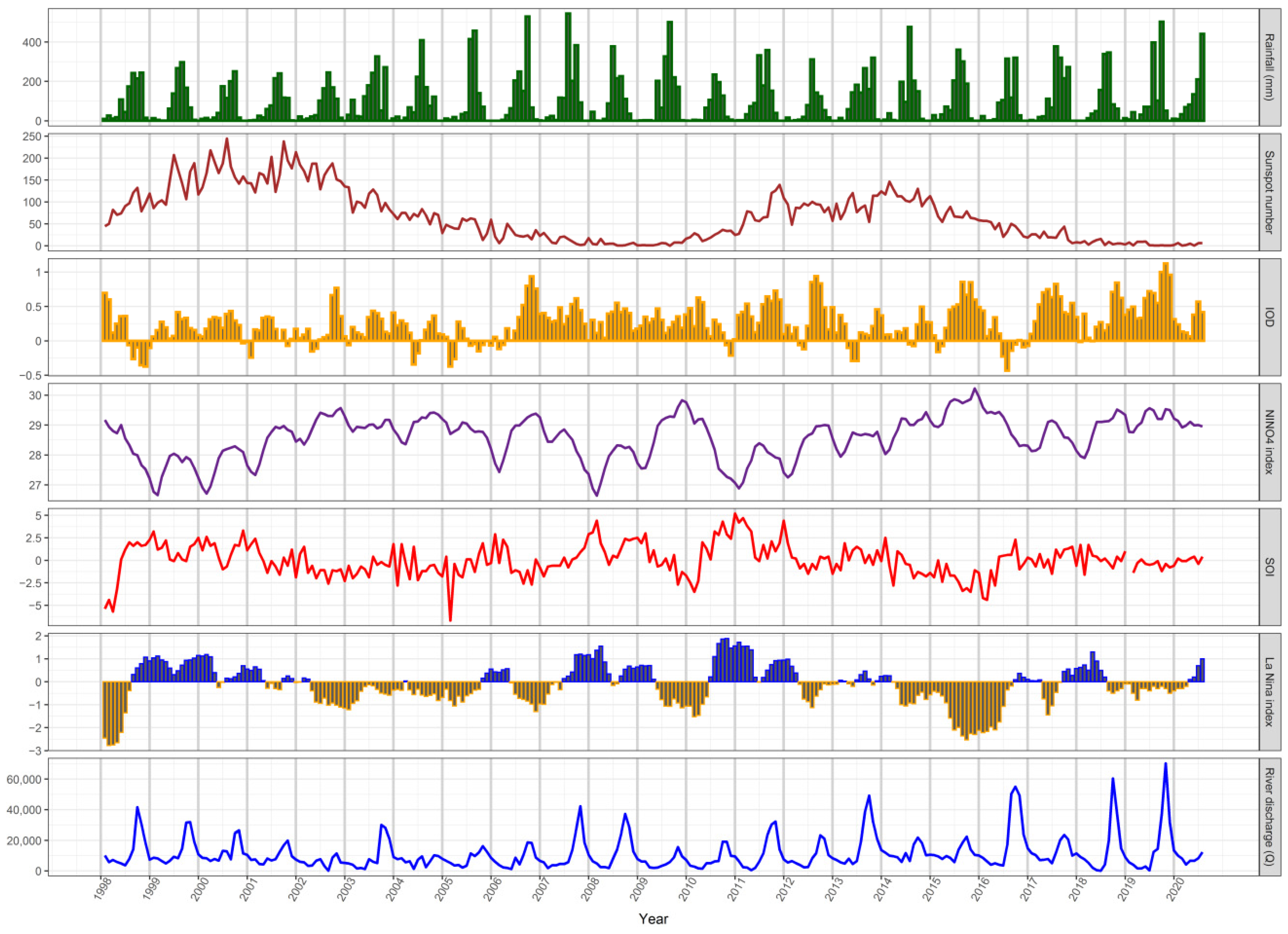
3.3. Long-Term Hydroclimatic Trends

JJAS rainfall reduced (Sen’s slope: −2.67, i.e., decrease of 2.67 mm/year over 50 years (CI95%: −1.68, −3.61), especially from 1959 onwards up to 2009 (Pettitt’s test for single-change-point detection: K = 2021, p < 0.0001). JJAS rainfall increased from 2010 onwards (Sen’s slope = 51.05 mm/year increase). The reduction in monsoonal rainfall at Bhagalpur became especially consistent from 1970 to 1971 onwards (in part explaining the decline in river discharge). An increasing but more variable trend in JFMAM rainfall was noted from 1975 onwards (Pettitt’s test: K = 757, p = 0.22). OND rainfall remained largely stable (Pettitt’s test: K = 547, p = 0.64). A clear relationship was estimated between channel width (W) measured in the field and from satellite images, and the natural logarithm of Manning’s equation-based discharge Q, as Q = exp(7.36–0.0023 × W); R2 = 0.81, p < 0.001, F = 30.07, df = 1, 7). We found a declining trend in estimated dry-season river discharge from 1972 onwards from channel widths measured from past images: Qyear = exp(67.725–0.029 × year); R2 = 0.67, p < 0.0001; F = 34.16, df = 1, 17). This translated to declining dry-season discharge at 2.86% per year.
From 2000 to 2020, we found a clear signal of increased variability in flood season river flow relative to dry-season low flows (flood amplitude) for the Ganga River (Figure 4 and Figure 5a). Two sunspot cycles were recorded in this period (Figure 4). An increase in dry-season flow, as well as flood season river flow, was seen especially after the 2010 El Niño event, after which the NINO4 index showed a hint of increase (Figure 4). Flood amplitude (i.e., flood-pulse strength) was the highest in moderate La Niña years but reduced during strong El Niño years (Figure 4). Negative and positive cross-correlations were seen between the NINO4 index and La Niña index with river flow, with lags of seven months and three months, respectively. However, the intra-annual seasonal variability in river discharge was also the highest during very strong El Niño (VSEL) years (Figure 5b). Flood amplitudes were highest in strong and moderate La Niña years (SLN, MLN) and reduced in years with weak to moderate El Niño (WEN and MEN) years but were highly variable in “very strong El-Niño” (VSEL) years. The sunspot cycle (of 11–13 years) showed two major phases in this period, a decline from 2000 to 2008 and a rise again in 2012–2014, followed by a consistent decline until 2020 (Figure 4). From 1998 to 2020, there was also a marked increase in flood-pulse duration from 2010 and advancement in flood rise timings (Figure 5c,d).

3.4. Long-Term Seasonal Trends in Fish Group Yields

Declining trends across the five fishery groups (carp, catfish, clupeids, others, shrimps), were pronounced for BGP (2000–2020) but not KHL (2013–2020) (Figure 6). Trends in fish group yields did not show significant trends in winter (JF) and monsoon (JJAS) seasons but declined in postmonsoon (OND) periods and summer (MAM) (Figure 6), which are both periods of high fishing activity. Statistically significant trends of decline were seen for carps (in MAM and OND), catfish (in MAM), clupeids (in JJAS and OND), and other fish and shrimp (in all seasons except JF). At Kahalgaon, significant declines were observed only for carps and clupeids in JJAS, while shrimps showed a recent increase in JJAS.

3.5. Responses of Fish Yields to Environmental Variability and Fishing Effort

At BGP, long-term aggregate yields of shrimps, other fish, and clupeids declined over time (Figure 7). Carp and catfish yields showed highly fluctuating behaviour but nonsignificant trends over time (Figure 7). Total fish yields declined from 2000 to 2006–2007 but then increased post-2008 and especially 2010 onwards, peaking in years with increasingly larger floods (Figure 4 and Figure 7). Major floods in 2008, 2011, 2013, 2016, and 2019 indicated a rough correspondence with the three-year major flooding recurrence. During years with stronger El Niño phases, the variability in yields was also greater, which appeared to be due to increasing variability in river flows after El Niño events (Figure 4 and Figure 7). For example, 2010 and 2015–2016 were strong El Niño events that led to poor summer fish yields but were followed by great floods in 2011 and 2016 that led to bumper yields. In turn, yields were higher after floods in weak to moderate La Niña years, as in 2008, 2013, and 2018 (Figure 4 and Figure 7), implying that productivity fluctuations are multiyear phenomena, dependent on strong flooding and periods of moderate drought.
At BGP, river flow was the predominant driver of yields of all fish groups (Table 2), followed by rainfall, which was negatively related with fish yields. Apart from river flow, monthly rainfall had a negative correlation with yields for all groups. All fish groups except carps and catfish declined over time, as seen from the nonsignificant trend effect (Table 2). Carp yields were lower in years with greater Indian Ocean Dipole activity and catfish yields in El Niño years (with high NINO4 values) (Table 2). For carp, catfish, and total catch, R2 values were moderate (>0.25), but for all other groups, low R2 values indicated weak but statistically significant relationships.
At KHL, river flow, fishing effort, and rainfall were the main predictors of total yields, but responses of catch per unit effort varied across groups. An interaction effect between river flow and fishing effort was detected as an important driver of fish group yields (Table 3). Catches per unit effort were negatively correlated with La Niña index (for carps and other fish), sunspot number (catfish and clupeids), and Indian Ocean Dipole index (carps, clupeids, shrimps) (Table 3). This indicated that catches per effort for carps, clupeids, and other fish were likely to intensify during stressful years (e.g., with El Niño droughts). Catches per unit effort were positively related to river flow (catfish) and rainfall (for shrimp and other fish) (Table 3). Low R2 values (<0.25) indicated weak but statistically significant relationships of catch per unit effort data with hydroclimatic variables for clupeid, others, shrimps, and total catch. Overall fishing effort was strongly dependent on river flow and La Niña index (Table 3), which was expected, as fishing effort closely tracked the flood-pulse strength in the postmonsoon peak fishing season (Figure 8). Total yields tracked changes in river flow. However, fishing effort was delinked from low dry-season flows and was greater during low-flow periods. Typically, at low river flows, fishing effort predicted yields, while at higher flows the effect of fishing effort on yields was weaker (Table 3). Fishing effort showed a significant declining trend (Table 3). Catches per unit effort (CPUE) were correlated with yields and effort at KHL from 2013 to 2020, barring an exceptional year of high catches during the El Niño drought in the summer of 2016 (Figure 9), but did not show statistically significant trends over time. At KHL, total yield and CPUE for fish groups did not show significant statistical trends over time (Mann–Kendall tests—total yield: tau = 0.06, p = 0.405; CPUE: tau = 0.114, p = 0.11), except for clupeids, which showed a declining trend (Table 3).

3.6. Fishing Behaviour and Hyperstability

At KHL, we found a strong signal of hyperstability from the total yield and catch-per-unit-effort (in terms of number of fisher days) relationship (β = 0.52 ± 0.05, log-log regression: R2 = 0.51, p < 0.001, F = 94.39, df = 1, 88). As we used fishery-dependent data for estimating yields, it is important to note that for hyperstable species, the observed catches could be masking the hydrologically driven trends of fish resource decline to some extent.
Overall, we found that (1) trends in yields of fishery groups were seasonally variable, but correlated with increasing flood-pulse variability, (2) both fishing effort and total yields responded similarly to river flow and flood-pulse strength, (3) fishing effort was strongly responsive to flooding but was decoupled from dry-season flow, and (4) catches per unit effort for all species combined did not show significant trends over time (Figure 9). These results suggest that trends in fishery yields may be driven by increasing hydrological variability in the monsoon and postmonsoon seasons and may be influenced by fishing intensity mainly during the dry season (Figure 8 and Figure 9).

4. Discussion

Our results imply that the positive effects of increasing flood magnitude on bumper fish yields may be countered by fishing effort when dry-season flows are reducing. However, as fishing effort has itself seen a declining trend in the last two decades, flood-pulse variability is the more significant driver of variability and uncertainty in fish yields as compared to the spatially localized effects of fishing pressure. With increasing variability in flood amplitude of the Ganga River, we show that the uncertainty in fish yields is also likely to increase. This finding is consistent with those of other studies on the Gangetic Plains. However, it does not support the perception of local fishers (which we had referred to as a “working hypothesis”) that overfishing is the ultimate cause of local fish declines and conflicts. The main message that emerges from our results is that the interplay of both factors needs to be further studied and addressed in the context of climate change and the impact of resource conflicts on fisher vulnerability. The BGP and KHL fisheries have been open access fisheries for three decades, and over time the number of fishers actively involved in fishing has reduced significantly. Many fishers have exited the fishery permanently out of distress due to conflict risks and fear from increasing control of anti-social elements [75]. Yet, at an aggregate level, it is difficult to say from the evidence available whether the Ganga River is “overfished” at present. Fish yields may well respond more strongly to recent environmental fluctuations as the total effort has declined [89,120].
This raises the question of how increasing uncertainty and extreme behaviour of river flows, linked with global climate change and anthropogenic perturbations at the basin scale, would drive fish yields in the near future. In this regard, there is scope for a better understanding of what overfishing would mean today, and under what conditions its impacts would be more severe than environmental impacts [121]. This is important because typically, overfishing is identified to be the reason for conflicts both by conservationists and development agencies, with a narrative based on “Malthusian overfishing” [122], while environmental variability and socioeconomic risks are seldom considered [123]. Fishers in pursuit of earning their livelihoods will have to deal more with increasing interannual uncertainty in fish yields caused by hydroclimatic variability, over and above their proximate concerns about declining catches.
That said, it is also true that the fishers that remain in the fishery continue to extract similar catches from a declining pool, even if the decline in yield is not entirely of their own doing. Those who remain have indeed intensified fishing efforts in terms of numbers of gears, nets, and time spent fishing, particularly in poor fishing years. What may not be “biological overfishing” might still become “socio-economic’” overfishing with the periodic intensification of “desperate” fishing in reaction to the high uncertainty in both dry-season “low flows” and flood season “highs”. Fishing has also been shifting towards smaller species caught with the use of passive traps and other stationary gears rather than active nets, which could cause changes in fish abundance and community composition in the near future. Thus, lagged recovery of larger species might occur due to shifts in relative fishing gear use. In this context, seasonal regulations on fishing effort may still be needed in the summer season (MAM) in particular [124]. We have shown that annual fishing effort typically increases when conditions support high productivity and reduces during conditions with poor productivity. Impacts of fishing are thus correlated with larger environmental impacts on fish yields. It could be that, as larger species have declined, smaller species, which are now the mainstay of the fishery, respond more sensitively to environmental variability (e.g., [32,125]).
Our study observes some curious patterns in fish yields with recent El Niño and La Niña events. In the period from 2002 to 2007, fish catches from Bhagalpur declined steadily during the weak ENSO phase that persisted over this time. From 2007 to 2008 and onwards though, fish yields picked up again in response to flood-pulses increasing in amplitude and showing greater extremes of variability. Fish yields showed declines in 2014-2015 and also responded negatively to the 2015-2016 ENSO drought, regarded as the fourth worst in 100 years [126], which nearly eliminated the flood-pulse in 2015. However, the strong flood-pulse in 2016 appears to have “reset” the fishery to its 2000 state. Chea et al. [127] have also noted such an effect of an extreme flooding event. By 2019–2020, fish yields appeared to be showing some recovery. However, such recovery might also be highly uncertain and noisy or flashy, occurring in phases of high and increasing environmental variability [128].
The peculiar circumstances of flooding in the Ganga in 2016 were in part due to rapid and abrupt large flow releases from dams on tributaries such as the Son. Long-term annual and seasonal rainfall (1991–2000) showed reductions [129,130], but more recent summer rainfall extremes and increases are becoming evident [70,131,132], whereas winter rainfall has shown declines [133] over eastern Bihar and the lower Gangetic Plains. The Son, in particular, has become an unpredictable and large contributor to flood season discharges in the Ganga. This change could be driven by the extremes of rainfall in central India [134], where the Son originates. Local precipitation recycling across North and Central India [135] could also be causing feedbacks between central Indian extreme rain events [136] and irrigation-induced weakening of summer monsoon rainfall in the Gangetic Plains [137]. Further, an increase in fine aerosol buildup in the middle and lower Gangetic Plains could alter rainfall intensity and magnitude [138,139]. This could aggravate tributary contributions (e.g., of the Son) to floods of the Ganga River in Bihar and increase fluctuations in fish yield dynamics in the near future. The Son discharges into the Ganga at Patna, and combined with the ponding effects of the downstream Farakka barrage, appear to have aggravated flooding in Bihar in recent years (https://sandrp.in/2016/08/23/a-tale-of-two-dams-is-bihars-unprecedented-flood-an-avoidable-man-made-disaster/ accessed on 30 September 2016). Mismatched timings of floodwater releases from the Farakka barrage and inflows from the Son and other tributaries could be responsible for large-scale flooding and inundation along Bihar’s floodplain region. Such dam-induced water releases do not carry sediment discharges that occur during natural flood-pulses. Dai et al. [100] had estimated a long-term decline in river flows at Farakka until 2004, but this pattern may now be reversing [140].
Fishery yields responded to increasing extremes of river discharges between the flood season and dry season [141]. Such enhanced or aseasonal fluctuations may affect the fisheries in the near future because of increasing uncertainty about equilibrium yields, resulting in fishers reluctant to invest further effort [120]. The frequency of severe droughts followed by severe floods in the Ganga in Bihar appears to be on the rise [142]. This pattern was noted in the four strongest ENSO years, which the active fishers we interviewed could still recall: 1970–1971, 1982–1983, 1997–1998, and 2015–2016. The effects of ENSO strength and sunspot activity were identified to drive not only fish yields but also determine fishing effort (during droughts) in our study area. With recurrences of El Niño droughts, effects of 11–13-year long sunspot cycles on fish species with spasmodic or irregular population recruitment dynamics may change [120,143]. These important hydroclimatic trends bear upon the proximate environmental cues that fish track during different stages of their life [25,144,145].
Dey et al. [17], in their documentation of fishers’ ecological knowledge from the same area, found that nonflood or year-round breeding fishes such as Cabdio morar (Danionidae) and Eutropichthys vacha (Ailiidae) had likely responded to such changes by modifying their reproductive responses to spawn multiple times every year. Evidence is emerging now that many species of the Gangetic Plains are changing their reproductive phenology, growth, and maturation patterns in response to climatic changes and fishing impacts (e.g., [31]: catfishes). Palaemonid shrimps could be sensitive to increased flooding pulses because their abundances peak in May-June, with increases in algal and decomposing organic matter. Smaller species, such as minnows, seem to be climate-resilient [32]. Clupeids, despite climatic change favourable to them, may not be able to sustain fishing pressures [61]. Species that reproduce in the dry season might not be affected by evolving climate trends [146].
Given that fishing practices in our study area are usually not selective towards particular species, the observation on hyperstability [117,147,148] needs to be considered further. Hyperstability may result from (1) diffuse fish stocks, as in many large rivers, and (2) stable fishing spots with nonrandom effort investment [13,119,148,149,150,151]. Aggregating, dispersing, or central-place space use by fish species could also affect these patterns [117]. Fishers reported that spots used by them stabilized in good years. In poorer years, effort investment became random and scattered, and at these times, catches may be proportional to yields. Fishing effort variation across years indicates a self-regulating effect of “effort sorting”, which appears adaptive to seasonally changing river flows [119,152]. Mobility of fishers in and out of the fishery is common, as they may seek to work as labourers elsewhere when returns become poor [153]. They may return for six months following a normal or “good” flood, because they are sure of making up for at least some of their investments. Usually, as fishing happens in dense clusters near fishing villages, exchanges through local fishers’ networks inform these decisions. Lagged effects of CPUFD at fixed fishing spots could lead to declining fish productivity in the subsequent dry season and aggravate conflicts. While our study identifies how aggregated fishing effort and yields respond to changing river flow regimes over time, one limitation is that it does not distinguish fish responses by different gear types, i.e., across active (e.g., gillnets) and passive gears (fish traps, baskets, stake nets, mosquito nets, etc.). A disaggregated analysis of how different gears affect catches and yields is out of the scope of the present study.
Since the fish declines seen from the 1970s onwards after the Farakka barrage, the BGP and KHL fisheries witnessed a shifted baseline. This could be another reason why local overfishing is the major cause perceived by fishers for increasing conflicts [17]. The relative contributions of environmental degradation (exogenous factors) and fishing (endogenous factors) on fish yields hold great relevance to the way these fisheries conflicts have been expressed [154,155]. They also influence prospects for ecosystem-based fisheries’ assessments and conservation [59,156,157]. Fishing effort can also change abruptly, facilitated by no barriers to exit or entry in the open access fishery. In the dry season of poor flow years, high fishing effort could have overwhelmed local fisheries’ productivity [158].
In the postmonsoon period of “good years”, fishers’ catches also increase as per productivity pulses and buffer them from the background threat of fish grabbing [159]. Better river flows increase the connectivity between side-channels and the main river, thus allowing increased access of fishers to productive fishing areas. In “bad years”, lateral disconnectivity and reduction in fish yields can not only affect fishers’ catches [160] but also make them more vulnerable to the threat of grabbing by other actors in the river floodplain (field observations). Local increases in fishing effort with improved river flow may be linked not only to greater resource availability but also to tracking greater availability of fishing space, with less potential for conflicts. Interannual changes in fishery yields thus create locally dynamic conditions that underlie how conflict situations are negotiated and adaptive strategies developed [25,161]. In summary, small-scale capture fisheries in the Gangetic Plains seem to be moving towards hydroclimatic regimes with high uncertainty and erratic perturbations to productivity, affecting the stability of fishing returns and risks of conflict. It is important for state fishery legislation and management policies to recognize these implications. In this context, restoring and managing ecological flow regimes and near-natural flow conditions at the river basin scale would be crucial to support fisheries’ productivity and livelihoods [8,20,162,163]. Water resource and fishery managers may not be able to respond to hydroclimatic uncertainty but can definitely work together to manage regulated river flows to maintain seasonally dynamic and adequate discharge in rivers to create conditions as close as possible to “normal” annual flood-pulses and low-flow regimes. Restoring annual flow patterns by providing near-natural flood-pulses, floodplain wetland restoration, and reoperation of dams and barrages to optimize water abstractions are all potential options to respond to increasing variability [20,21]. Such attempts at restoration of fish habitats can provide gainful returns from fishers’ catches and help them better adapt to shocks and perturbations from increasing hydroclimatic variability.

Author Contributions

Conceptualization, N.K, J.K., R.A., S.D.; methodology, N.K., J.K., R.A., S.D.; software, N.K., J.K.; validation, N.K., J.K., R.A., S.D.; formal analysis, N.K., J.K.; investigation, N.K., S.D.; resources, N.K., J.K.; data curation, N.K., S.D.; writing—original draft preparation, N.K.; writing—review and editing, N.K., R.A., J.K., S.D.; visualization, N.K., R.A., J.K.; supervision, J.K., R.A.; project administration, N.K., J.K.; funding acquisition, N.K., J.K. All authors have read and agreed to the published version of the manuscript.

Funding

N.K. was funded by the Tata Trusts, the International Whaling Commission Small Cetacean Research Fund (2013–2016), Duleep Matthai Nature Conservation Trust (2015–2017, 2019–2021), and New India Foundation, and ATREE. N.K. and S.D. were supported by BNP Paribas India Foundation, DSP HMK Holdings Pvt. Ltd., and the Wildlife Conservation Trust. R.A. thanks the Cholamandalam Investment and Finance Company, Shri Amm Murugappa Chettiar Research Centre, and Arvind Dattar for funding support. J.K. thanks the Biodiversity Collaborative, and the MoES-NERC Newton-Bhabha Sustaining Water Resources Fund for funding support.

Institutional Review Board Statement

Ethical approval for the study was provided by the ATREE Academy for Conservation and Sustainability Studies to N.K. A number was not assigned as the Institutional Review Board was to be reconvened at the time of submission. Additionally, due to the fact that fishers were known to N.K. and S.D. for over a decade and had participated voluntarily in the fish catch-effort data collection and had regularly shared their observations of change and related insights with us over a long time.

Informed Consent Statement

Informed consent was verbally obtained from all human subjects involved in the study. Fishers voluntarily participated in the study and were personally known to us for a long time.

Data Availability Statement

The fisheries data and hydrological data collected by the authors, and presented in this study may be made available on request by the corresponding author. The data on fishers’narratives cannot be shared as they may have confidential information that will not be disclosed. Data sources for hydro-climatic variables are clearly indicated in the paper through website links, all of which are open to public access and use.

Acknowledgments

This paper is based on a part of the Ph.D. thesis (URL: https://shodhganga.inflibnet.ac.in/handle/10603/341353, accessed on 19 December 2021) of the lead and corresponding author Nachiket Kelkar (N.K.) at the Ashoka Trust for Research in Ecology and the Environment (ATREE), for which the degree was awarded by the Manipal Academy of Higher Education, Manipal, in 2021. N.K. was guided by Jagdish Krishnaswamy and Rohan Arthur was a Doctoral Advisory Committee Member. We also thank N.K.’s Doctoral Advisory Committee members Siddhartha Krishnan and Rohan D’Souza for their intellectual inputs on some ideas discussed in the paper, and Sunil Kumar Choudhary for his vision and constant support to the long-term fisheries monitoring programme. We thank all fishers and fish traders who helped us in data collection, and who also kindly and voluntarily shared fish catch-effort and market logbook data with us. All data collection was carried out only with prior verbal consent of the fishers involved, facilitated by our long-term association with them. We thank ATREE, Bangalore, for the institutional and academic support they provided for this work. N.K. thanks the Tata Trusts, the International Whaling Commission Small Cetacean Research Fund (2013–2016), Duleep Matthai Nature Conservation Trust (2015–2017, 2019–2021), New India Foundation, BNP Paribas India Foundation, DSP HMK Holdings Pvt. Ltd., and the Wildlife Conservation Trust for funding support. J.K.’s contribution was partially supported and catalyzed by the Office of the Principal Scientific Adviser to the Government of India through a grant to the Biodiversity Collaborative. R.A. thanks the Cholamandalam Investment and Finance Company, Shri Amm Murugappa Chettiar Research Centre, and Arvind Dattar for funding support.

Conflicts of Interest

The authors declare no conflict of interest.

References

  1. Smith, L.E.D.; Khoa, S.N.; Lorenzen, K. Livelihood functions of inland fisheries: Policy implications in developing countries. Water Policy 2005, 7, 359–383. [Google Scholar] [CrossRef]
  2. Lynch, A.J.; Cooke, S.J.; Deines, A.M.; Bower, S.D.; Bunnell, D.B.; Cowx, I.G.; Nguyen, V.M.; Nohner, J.; Phouthavong, K.; Riley, B.; et al. The social, economic, and environmental importance of inland fish and fisheries. Environ. Rev. 2016, 24, 115–121. [Google Scholar] [CrossRef] [Green Version]
  3. Funge-Smith, S.; Bennett, A. A fresh look at inland fisheries and their role in food security and livelihoods. Fish Fish. 2019, 20, 1176–1195. [Google Scholar] [CrossRef] [Green Version]
  4. Humphries, P.; King, A.J.; Koehn, J.D. Fish, flows and flood plains: Links between freshwater fishes and their environment in the Murray-Darling River system, Australia. Environ. Biol. Fishes 1999, 56, 129–151. [Google Scholar] [CrossRef]
  5. Tockner, K.; Stanford, J.A. Riverine flood plains: Present state and future trends. Environ. Conserv. 2002, 29, 308–330. [Google Scholar] [CrossRef] [Green Version]
  6. Agostinho, A.A.; Gomes, L.C.; Veríssimo, S.; Okada, E.K. Flood regime, dam regulation and fish in the Upper Paraná River: Effects on assemblage attributes, reproduction and recruitment. Rev. Fish Biol. Fish. 2004, 14, 11–19. [Google Scholar] [CrossRef]
  7. Dudgeon, D. River Rehabilitation for Conservation of Fish Biodiversity in Monsoonal Asia. Ecol. Soc. 2005, 10, 15. [Google Scholar] [CrossRef]
  8. Dudgeon, D.; Arthington, A.H.; Gessner, M.O.; Kawabata, Z.I.; Knowler, D.J.; Lévêque, C.; Naiman, R.J.; Prieur-Richard, A.H.; Soto, D.; Stiassny, M.L.; et al. Freshwater biodiversity: Importance, threats, status and conservation challenges. Biol. Rev. 2006, 81, 163–182. [Google Scholar] [CrossRef]
  9. Humphries, P.; Richardson, A.; Wilson, G.; Ellison, T. River regulation and recruitment in a protracted-spawning riverine fish. Ecol. Appl. 2013, 23, 208–225. [Google Scholar] [CrossRef] [Green Version]
  10. Masood, M.; Yeh, P.J.-F.; Hanasaki, N.; Takeuchi, K. Model study of the impacts of future climate change on the hydrology of Ganges–Brahmaputra–Meghna basin. Hydrol. Earth Syst. Sci. 2015, 19, 747–770. [Google Scholar] [CrossRef] [Green Version]
  11. Whitehead, P.G.; Barbour, E.; Futter, M.N.; Sarkar, S.; Rodda, H.; Caesar, J.; Butterfield, D.; Jin, L.; Sinha, R.; Nicholls, R.; et al. Impacts of climate change and so-cio-economic scenarios on flow and water quality of the Ganges, Brahmaputra and Meghna (GBM) river systems: Low flow and flood statistics. Environ. Sci. Process. Impacts 2015, 17, 1057–1069. [Google Scholar] [CrossRef] [PubMed]
  12. Anand, J.; Gosain, A.K.; Khosa, R.; Srinivasan, R. Regional scale hydrologic modeling for prediction of water balance, analysis of trends in streamflow and variations in streamflow: The case study of the Ganga River basin. J. Hydrol. Reg. Stud. 2018, 16, 32–53. [Google Scholar] [CrossRef]
  13. Welcomme, R.L. Inland Fisheries: Ecology and Management; Blackwell Science for Food and Agriculture Organization of the United Nations: Ames, IN, USA, 2002. [Google Scholar]
  14. Welcomme, R.L.; Cowx, I.G.; Coates, D.; Béné, C.; Funge-Smith, S.; Halls, A.; Lorenzen, K. Inland capture fisheries. Philos. Trans. R. Soc. B Biol. Sci. 2010, 365, 2881–2896. [Google Scholar] [CrossRef] [PubMed]
  15. De Graaf, G. The flood pulse and growth of floodplain fish in Bangladesh. Fish. Manag. Ecol. 2003, 10, 241–247. [Google Scholar] [CrossRef]
  16. Rodríguez, M.A.; Winemiller, K.O.; Lewis, W.M., Jr.; Taphorn Baechle, D.C. The freshwater habitats, fishes, and fisheries of the Orinoco River basin. Aquat. Ecosyst. Health Manag. 2007, 10, 140–152. [Google Scholar] [CrossRef]
  17. Dey, S.; Choudhary, S.K.; Dey, S.; Deshpande, K.; Kelkar, N. Identifying potential causes of fish declines through local ecological knowledge of fishers in the Ganga River, eastern Bihar, India. Fish. Manag. Ecol. 2020, 27, 140–154. [Google Scholar] [CrossRef]
  18. Bayazit, M. Nonstationarity of hydrological records and recent trends in trend analysis: A state-of-the-art review. Environ. Process. 2015, 2, 527–542. [Google Scholar] [CrossRef]
  19. Krishnaswamy, J.; Vaidyanathan, S.; Rajagopalan, B.; Bonell, M.; Sankaran, M.; Bhalla, R.S.; Badiger, S. Non-stationary and non-linear influence of ENSO and Indian Ocean Dipole on the variability of Indian monsoon rainfall and extreme rain events. Clim. Dyn. 2015, 45, 175–184. [Google Scholar] [CrossRef]
  20. Humphries, P.; Winemiller, K.O. Historical Impacts on River Fauna, Shifting Baselines, and Challenges for Restoration. BioScience 2009, 59, 673–684. [Google Scholar] [CrossRef] [Green Version]
  21. Bladon, A.J.; Mohammed, E.Y.; Ali, L.; Milner-Gulland, E.J. Developing a frame of reference for fisheries management and conservation interventions. Fish. Res. 2018, 208, 296–308. [Google Scholar] [CrossRef]
  22. Ngor, P.B.; McCann, K.S.; Grenouillet, G.; So, N.; McMeans, B.C.; Fraser, E.; Lek, S. Evidence of indiscriminate fishing effects in one of the world’s largest inland fisheries. Sci. Rep. 2018, 8, 8947. [Google Scholar] [CrossRef] [Green Version]
  23. De Graaf, G.; Bartley, D.; Jorgensen, J.; Marmulla, G. The scale of inland fisheries, can we do better? Alternative approaches for assessment. Fish. Manag. Ecol. 2015, 22, 64–70. [Google Scholar] [CrossRef]
  24. Myers, B.J.E.; Lynch, A.J.; Bunnell, D.B.; Chu, C.; Falke, J.A.; Kovach, R.P.; Krabbenhoft, T.J.; Kwak, T.; Paukert, C.P. Global synthesis of the documented and projected effects of climate change on inland fishes. Rev. Fish Biol. Fish. 2017, 27, 339–361. [Google Scholar] [CrossRef]
  25. Keyl, F.; Wolff, M. Environmental variability and fisheries: What can models do? Rev. Fish Biol. Fish. 2008, 18, 273–299. [Google Scholar] [CrossRef]
  26. Gamble, R.J.; Link, J.S. Analyzing the tradeoffs among ecological and fishing effects on an example fish community: A multispecies (fisheries) production model. Ecol. Model. 2009, 220, 2570–2582. [Google Scholar] [CrossRef]
  27. Ahmed, K.K.U.; Ahmed, S.U.; Haldar, G.C.; Hossain, M.R.A.; Ahmed, T. Primary Production and Fish Yield Estimation in the Meghna River System, Bangladesh. Asian Fish. Sci. 2005, 18, 95. [Google Scholar] [CrossRef]
  28. Hilborn, R.; Quinn, T.P.; Schindler, D.E.; Rogers, D.E. Biocomplexity and fisheries sustainability. Proc. Natl. Acad. Sci. USA 2003, 100, 6564–6568. [Google Scholar] [CrossRef] [Green Version]
  29. Baran, E. Fish migration triggers in the Lower Mekong Basin and other tropical freshwater systems. MRC Tech. Pap. 2006, 14, 55. [Google Scholar]
  30. Das, M.K.; Sharma, A.P.; Sahu, S.K.; Srivastava, P.K.; Rej, A. Impacts and vulnerability of inland fisheries to climate change in the Ganga River system in India. Aquat. Ecosyst. Health Manag. 2013, 16, 415–424. [Google Scholar] [CrossRef]
  31. Sarkar, U.K.; Naskar, M.; Roy, K.; Sudeeshan, D.; Srivastava, P.; Gupta, S.; Bose, A.K.; Verma, V.K.; Das Sarkar, S.; Karnatak, G.; et al. Benchmarking pre-spawning fitness, climate preferendum of some catfishes from river Ganga and its proposed utility in climate research. Environ. Monit. Assess. 2017, 189, 491. [Google Scholar] [CrossRef]
  32. Sarkar, U.K.; Roy, K.; Naskar, M.; Srivastava, P.K.; Bose, A.K.; Verma, V.K.; Gupta, S.; Nandy, S.K.; Das Sarkar, S.; Karnatak, G.; et al. Minnows may be more reproductively resilient to climatic variability than anticipated: Synthesis from a reproductive vulnerability assessment of Gangetic pool barbs (Puntius sophore). Ecol. Indic. 2019, 105, 727–736. [Google Scholar] [CrossRef]
  33. Jul-Larsen, E. (Ed.) Management, Co-Management, or no Management? Major Dilemmas in Southern African Freshwater Fisheries; Food & Agriculture Organization: Rome, Italy, 2003. [Google Scholar]
  34. Junk, W.J.; Bayley, P.B.; Sparks, R.E. The flood pulse concept in river-floodplain systems. Can. Spec. Publ. Fish. Aquat. Sci. 1989, 106, 110–127. [Google Scholar]
  35. Humphries, P.; Keckeis, H.; Finlayson, B. The River Wave Concept: Integrating River Ecosystem Models. BioScience 2014, 64, 870–882. [Google Scholar] [CrossRef]
  36. Tockner, K.; Malard, F.; Ward, J.V. An extension of the flood pulse concept. Hydrol. Process. 2000, 14, 2861–2883. [Google Scholar] [CrossRef]
  37. Thorp, J.H.; Thoms, M.C.; Delong, M.D. The riverine ecosystem synthesis: Biocomplexity in river networks across space and time. River Res. Appl. 2006, 22, 123–147. [Google Scholar] [CrossRef]
  38. Baran, E.; van Zalinge, N.; Ngor, P.B. Floods, floodplains, and fish production in the Mekong Basin: Present and past trends. In Proceedings of the second Asian wetlands symposium, Penang, Malaysia, 27–30 August 2001; Ahyaudi, A., Ed.; Penerbit Universiti Sains Malaysia: Pulau Pinang, Malaysia, 2001; pp. 920–932. [Google Scholar]
  39. Graham, R.; Harris, J.H. Floodplain Inundation and Fish Dynamics in the Murray-Darling Basin: Current Concepts and Future Research: A Scoping Study; CRC for Freshwater Ecology: Canberra, Australia, 2005; 56p. [Google Scholar]
  40. Cloern, J.E. Habitat connectivity and ecosystem productivity: Implications from a simple model. Am. Nat. 2007, 169, E21–E33. [Google Scholar] [CrossRef]
  41. Lyon, J.; Stuart, I.; Ramsey, D.; O’Mahony, J. The effect of water level on lateral movements of fish between river and off-channel habitats and implications for management. Mar. Freshw. Res. 2010, 61, 271–278. [Google Scholar] [CrossRef] [Green Version]
  42. Rolls, R.J.; Growns, I.O.; Khan, T.A.; Wilson, G.G.; Ellison, T.L.; Prior, A.; Waring, C.C. Fish recruitment in rivers with modified discharge depends on the interacting effects of flow and thermal regimes. Freshw. Biol. 2013, 58, 1804–1819. [Google Scholar] [CrossRef]
  43. Qasim, S.Z.; Qayyum, A. Spawning frequencies and breeding seasons of some freshwater fishes with special reference to those occurring in the plains of northern India. Indian J. Fish. 1962, 8, 24–43. [Google Scholar]
  44. King, A.J.; Humphries, P.; Lake, P.S. Fish recruitment on floodplains: The roles of patterns of flooding and life history characteristics. Can. J. Fish. Aquat. Sci. 2003, 60, 773–786. [Google Scholar] [CrossRef]
  45. Payne, A.I.; Sinha, R.; Singh, H.R.; Huq, S. A review of the Ganges Basin: Its fish and fisheries. In Proceedings of the Second International Symposium on the Management of Large Rivers for Fisheries, Phnom Penh, Cambodia, 11–14 February 2003; Welcomme, R.L., Peter, T., Eds.; FAO: Bangkok, Thailand, 2004; Volume 1, pp. 229–250. [Google Scholar]
  46. Vilizzi, L. Abundance trends in floodplain fish larvae: The role of annual flow characteristics in the absence of overbank flooding. Fundam. Appl. Limnol. Arch. Furhydrobiologie 2012, 181, 215–227. [Google Scholar] [CrossRef]
  47. Das, M.K.; Srivastava, P.K.; Rej, A.; Mandal, L.; Sharma, A.P. A framework for assessing vulnerability of inland fisheries to impacts of climate variability in India. Mitig. Adapt. Strat. Glob. Chang. 2016, 21, 279–296. [Google Scholar] [CrossRef]
  48. Walton, S.E.; Nunn, A.D.; Probst, W.N.; Bolland, J.D.; Acreman, M.; Cowx, I.G. Do fish go with the flow? The effects of periodic and episodic flow pulses on 0+ fish biomass in a constrained lowland river. Ecohydrology 2017, 10, e1777. [Google Scholar] [CrossRef]
  49. Bernhardt, J.R.; O’Connor, M.I.; Sunday, J.M.; Gonzalez, A. Life in fluctuating environments. Philos. Trans. R. Soc. B 2020, 375, 20190454. [Google Scholar] [CrossRef] [PubMed]
  50. Sinha, M.; Khan, M.A.; Jha, B.C. (Eds.) Ecology, Fisheries and Fish-Stock Assessment of Indian Rivers; Bulletin No. 90; CIFRI: Barrackpore, India, 1999; 325p. [Google Scholar]
  51. Sinha, M.; Khan, M.A. Impact of environmental aberrations on fisheries of the Ganga (Ganges) River. Aquat. Ecosyst. Health Manag. 2001, 4, 493–504. [Google Scholar] [CrossRef]
  52. Halls, A.S.; Welcomme, R.L. Dynamics of river fish populations in response to hydrological conditions: A simulation study. River Res. Appl. 2004, 20, 985–1000. [Google Scholar] [CrossRef]
  53. Halls, A.S.; Welcomme, R.L.; Burn, R.W. The relationship between multi-species catch and effort: Among fishery comparisons. Fish. Res. 2006, 77, 78–83. [Google Scholar] [CrossRef]
  54. Vass, K.K.; Mondal, S.K.; Samanta, S.; Suresh, V.R.; Katiha, P.K. The environment and fishery status of the River Ganges. Aquat. Ecosyst. Health Manag. 2010, 13, 385–394. [Google Scholar] [CrossRef]
  55. Castello, L.; McGrath, D.G.; Beck, P.S. Resource sustainability in small-scale fisheries in the Lower Amazon floodplains. Fish. Res. 2011, 110, 356–364. [Google Scholar] [CrossRef]
  56. FAO and WorldFish Center. Small-Scale Capture Fisheries: A Global Overview with Emphasis on Developing Countries; WorldFish: Penang, Malaysia, 2008. [Google Scholar]
  57. Bartley, D.M.; De Graaf, G.; Valbo-Jørgensen, J.; Marmulla, G. Inland capture fisheries: Status and data issues. Fish. Manag. Ecol. 2015, 22, 71–77. [Google Scholar] [CrossRef]
  58. Baran, E.; Myschowoda, C. Have fish catches been declining in the Mekong River Basin? In Moderns Myths of the Mekong; Kummu, M., Keskinen, M., Varis, O., Eds.; Water and Development Pubs: Helsinki, Finland, 2008; pp. 55–64. [Google Scholar]
  59. Campbell, I.C. Perceptions, data, and river management: Lessons from the Mekong River. Water Resour. Res. 2007, 43. [Google Scholar] [CrossRef] [Green Version]
  60. Government of India. Manual on Fishery Statistics. Section B—Inland Fishery; Ministry of Statistics and Program Implementation, Central Statistics Office, Govt. of India: New Delhi, India, 2021. [Google Scholar]
  61. Sarkar, U.K.; Roy, K.; Karnatak, G.; Naskar, M.; Puthiyottil, M.; Baksi, S.; Lianthuamluaia, L.; Kumari, S.; Ghosh, B.D.; Das, B.K. Reproductive environment of the decreasing Indian river shad in Asian inland waters: Disentangling the climate change and indiscriminative fishing threats. Environ. Sci. Pollut. Res. 2021, 28, 30207–30218. [Google Scholar] [CrossRef] [PubMed]
  62. Armstrong, R.L.; Rittger, K.; Brodzik, M.J.; Racoviteanu, A.; Barrett, A.P.; Khalsa, S.-J.S.; Raup, B.; Hill, A.; Khan, A.; Wilson, A.M.; et al. Runoff from glacier ice and seasonal snow in High Asia: Separating melt water sources in river flow. Reg. Environ. Chang. 2019, 19, 1249–1261. [Google Scholar] [CrossRef] [Green Version]
  63. Sarkar, U.K.; Pathak, A.K.; Sinha, R.K.; Sivakumar, K.; Pandian, A.K.; Pandey, A.; Dubey, V.K.; Lakra, W.S. Freshwater fish biodiversity in the River Ganga (India): Changing pattern, threats and conservation perspectives. Rev. Fish Biol. Fish. 2012, 22, 251–272. [Google Scholar] [CrossRef]
  64. Das, M.K.; Samanta, S.; Saha, P.K. Riverine Health and Impact on Fisheries in India; Policy Paper No. 01; Central Inland Fisheries Research Institute: Barrackpore, Kolkata, 2007; p. 120. [Google Scholar]
  65. Jhingran, A.G.; Ghosh, K.K. The fisheries of the Ganga River System in the context of Indian aquaculture. Aquaculture 1978, 14, 141–162. [Google Scholar] [CrossRef]
  66. Talwar, P.K.; Jhingran, A.G. Inland Fishes of India and Adjacent Countries; Oxford and IBH Publishing Co.: New Delhi, India; Bombay, India; Calcutta, India, 1991; Volume 1–2, 1158p. [Google Scholar]
  67. Ray, P. Ecological Imbalance of the Ganga River System: Its Impact on Aquaculture; Daya Books: Delhi, India, 1998; pp. 198–226. [Google Scholar]
  68. Vass, K.K.; Das, M.K.; Srivastava, P.K.; Dey, S. Assessing the impact of climate change on inland fisheries in River Ganga and its plains in India. Aquat. Ecosyst. Health Manag. 2009, 12, 138–151. [Google Scholar] [CrossRef]
  69. Vass, K.K.; Tyagi, R.K.; Singh, H.P.; Pathak, V. Ecology, changes in fisheries, and energy estimates in the middle stretch of the River Ganges. Aquat. Ecosyst. Health Manag. 2010, 13, 374–384. [Google Scholar] [CrossRef]
  70. Das, B.K.; Sarkar, U.K.; Roy, K. Global Climate Change and Inland Open Water Fisheries in India: Impact and Adaptations; Climate Change and Agriculture in India: Impact and Adaptation; Central Inland Fisheries Research Institute: Barrackpore, West Bengal, India, 2019; pp. 79–95. [Google Scholar]
  71. CIFRI. Inland Fisheries and Climate Change: Vulnerability and Adaptation Options; ICAR-CIFRI Special Publication, Policy Paper No. 2015-1611; ICAR-CIFRI: Barrackpore, India, 2015; ISSN 0970-616X. [Google Scholar]
  72. Datta Munshi, J.; Bilgrami, K.S.; Saha, M.P.; Johar, M.A. Survey of fish-spawn collection grounds in the river Ganges. Environ. Conserv. 1979, 6, 153–157. [Google Scholar] [CrossRef]
  73. Rahman, M.; Rahaman, M.M. Impacts of Farakka barrage on hydrological flow of Ganges river and environment in Bangladesh. Sustain. Water Resour. Manag. 2018, 4, 767–780. [Google Scholar] [CrossRef]
  74. Choudhary, S.K.; Dey, S.; Kelkar, N. Locating fisheries and livelihood issues in river biodiversity conservation: Insights from long-term engagement with fisheries in the Vikramshila Gangetic Dolphin Sanctuary riverscape, Bihar, India. In Proceedings of the IUCN Symposium on Riverine Biodiversity, Patna, India, 4–6 April 2014. [Google Scholar]
  75. Kelkar, N.; Dey, S. On Temperaments, Communities, and Conflicts in the River Fisheries of Bihar, Amidst Rigidly Persistent Caste and Class Discrimination; Samudra Newsletter; International Collective in Support of Fishworkers (ICSF): Chennai, India, 2016; Volume 75, pp. 72–75. [Google Scholar]
  76. Kelkar, N. The resource of tradition: Changing identities and conservation conflicts in Gangetic fisheries. In Conservation from the Margins; Srinivasan, U., Velho, N., Eds.; Orient BlackSwan: Hyderabad, India, 2018; pp. 9–32. [Google Scholar]
  77. Montaña, C.G.; Choudhary, S.K.; Dey, S.; Winemiller, K.O. Compositional trends of fisheries in the River Ganges, India. Fish. Manag. Ecol. 2011, 18, 282–296. [Google Scholar] [CrossRef]
  78. Choudhary, S.K.; Smith, B.D.; Dey, S.; Dey, S.; Prakash, S. Conservation and biomonitoring in the Vikramshila Gangetic Dolphin Sanctuary, Bihar, India. Oryx 2006, 40, 189–197. [Google Scholar] [CrossRef] [Green Version]
  79. Sharma, A.P.; Katiha, P.K.; Sahoo, A.K.; Chandra, G. State of Inland Fisheries and Inland Fisher Community of India; FAO Bay of Bengal Project Report; CIFRI: Barrackpore, West Bengal, India, 2013; 21p. [Google Scholar]
  80. Narayanan, S. Inland Fisheries, Food Security, and Poverty Eradication: A Case Study of Bihar and West Bengal; International Collective in Support of Fishworkers (ICSF) Occasional Paper; International Collective in Support of Fishworkers: Chennai, India, 2016; 59+vi p. [Google Scholar]
  81. India Meteorological Department (IMD). Ministry of Earth Sciences, Gov. of India. Available online: https://www.imd.gov.in (accessed on 15 October 2021).
  82. Singh, M.; Singh, I.B.; Müller, G. Sediment characteristics and transportation dynamics of the Ganga River. Geomorphology 2007, 86, 144–175. [Google Scholar] [CrossRef]
  83. Hooke, J. River meander behaviour and instability: A framework for analysis. Trans. Inst. Br. Geogr. 2003, 28, 238–253. [Google Scholar] [CrossRef]
  84. Mirza, M.M.Q. Hydrological changes in the Ganges system in Bangladesh in the post-Farakka period. Hydrol. Sci. J. 1997, 42, 613–631. [Google Scholar] [CrossRef]
  85. Adel, M.M. Effect on Water Resources from Upstream Water Diversion in the Ganges Basin. J. Environ. Qual. 2001, 30, 356–368. [Google Scholar] [CrossRef]
  86. Kawser, M.A.; Samad, M.A. Political history of Farakka barrage and its effects on environment in Bangladesh. Bandung 2016, 3, 1–4. [Google Scholar] [CrossRef] [Green Version]
  87. Sparre, P.; Venema, S.C. Introduction to Tropical Fish STOCK Assessment, Part I: Manua. FAO Fisheries Technical Paper 306. 1998. Available online: http://www.fao.org/docrep/w5449e/w5449e00.htm (accessed on 20 May 2018).
  88. Lorenzen, K.; Almeida, O.; Arthur, R.; Garaway, C.; Khoa, S.N. Aggregated yield and fishing effort in multispecies fisheries: An empirical analysis. Can. J. Fish. Aquat. Sci. 2006, 63, 1334–1343. [Google Scholar] [CrossRef] [Green Version]
  89. Lorenzen, K.; Cowx, I.G.; Entsua-Mensah, R.E.M.; Lester, N.P.; Koehn, J.D.; Randall, R.G.; So, N.; Bonar, S.A.; Bunnell, D.B.; Venturelli, P.; et al. Stock assessment in in-land fisheries: A foundation for sustainable use and conservation. Rev. Fish Biol. Fish. 2016, 26, 405–440. [Google Scholar] [CrossRef]
  90. Welcomme, R.L. Data requirements for inland fisheries management. In New Approaches for the Improvement of Inland Capture Fishery Statistics in the Mekong Basin; FAO: Rome, Italy; Mekong River Commission: Vientiane, Laos; Govt. of Thailand: Bangkok, Thailand, 2003; Available online: http://www.fao.org/docrep/005/ad070e/ad070e09.htm#bm9 (accessed on 27 July 2018).
  91. Bishop, J. Standardizing fishery-dependent catch and effort data in complex fisheries with technology change. Rev. Fish Biol. Fish. 2006, 16, 21–38. [Google Scholar] [CrossRef]
  92. Maunder, M.N.; Sibert, J.R.; Fonteneau, A.; Hampton, J.; Kleiber, P.; Harley, S.J. Interpreting catch per unit effort data to assess the status of individual stocks and communities. Ices J. Mar. Sci. 2006, 63, 1373–1385. [Google Scholar] [CrossRef]
  93. Maunder, M.N.; Punt, A.E. A review of integrated analysis in fisheries stock assessment. Fish. Res. 2013, 142, 61–74. [Google Scholar] [CrossRef]
  94. Pope, K.L.; Willis, D.W. Seasonal influences on freshwater fisheries sampling data. Rev. Fish. Sci. 1996, 4, 57–73. [Google Scholar] [CrossRef] [Green Version]
  95. Johnson, A.F.; Moreno-Báez, M.; Giron-Nava, A.; Corominas, J.; Erisman, B.; Ezcurra, E.; Aburto-Oropeza, O. A spatial method to calculate small-scale fisheries effort in data poor scenarios. PLoS ONE 2017, 12, e0174064. [Google Scholar] [CrossRef] [PubMed] [Green Version]
  96. Brakenridge, G.R.; Kettner, A.; Syvitski, J.; Overeem, I.; De Groeve, T.; Cohen, S.; Nghiem, S.V. Experimental Satel-Lite-Based River Discharge Measurements: Technical Summary (River Watch Version 3.4). 2017. Available online: http://floodobservatory.colorado.edu/satellitegaugingsites/technical.html (accessed on 31 December 2020).
  97. Chow, V.T. Open-Channel Hydraulics; McGraw-Hill: New York, NY, USA, 1959; 680p. [Google Scholar]
  98. Williams, G.P. Bank-full discharge of rivers. Water Resour. Res. 1978, 14, 1141–1154. [Google Scholar] [CrossRef]
  99. Arcement, G.J.; Schneider, V.R. Guide for Selecting Manning’s Roughness Coefficients for Natural Channels and Floodplains; Water-Supply Paper 23; United States Geological Survey: Reston, VA, USA, 1989; 39p. [Google Scholar]
  100. Dai, A.; Qian, T.; Trenberth, K.E.; Milliman, J.D. Changes in Continental Freshwater Discharge from 1948 to 2004. J. Clim. 2009, 22, 2773–2792. [Google Scholar] [CrossRef]
  101. Pavelsky, T.M. Using width-based rating curves from spatially discontinuous satellite imagery to monitor river discharge. Hydrol. Process. 2014, 28, 3035–3040. [Google Scholar] [CrossRef]
  102. Sichangi, A.W.; Wang, L.; Hu, Z. Estimation of River Discharge Solely from Remote-Sensing Derived Data: An Initial Study Over the Yangtze River. Remote Sens. 2018, 10, 1385. [Google Scholar] [CrossRef] [Green Version]
  103. Yamazaki, D.; O’Loughlin, F.; Trigg, M.A.; Miller, Z.F.; Pavelsky, T.M.; Bates, P.D. Development of the Global Width Database for Large Rivers. Water Resour. Res. 2014, 50, 3467–3480. [Google Scholar] [CrossRef]
  104. Pekel, J.-F.; Cottam, A.; Gorelick, N.; Belward, A.S. High-resolution mapping of global surface water and its long-term changes. Nature 2016, 540, 418–422. [Google Scholar] [CrossRef]
  105. Ward, P.J.; Beets, W.; Bouwer, L.M.; Aerts, J.C.J.H.; Renssen, H. Sensitivity of river discharge to ENSO. Geophys. Res. Lett. 2010, 37, L12402. [Google Scholar] [CrossRef] [Green Version]
  106. Pervez, M.S.; Henebry, G.M. Spatial and seasonal responses of precipitation in the Ganges and Brahmaputra river basins to ENSO and Indian Ocean dipole modes: Implications for flooding and drought. Nat. Hazards Earth Syst. Sci. 2015, 15, 147–162. [Google Scholar] [CrossRef] [Green Version]
  107. Pokhrel, S.; Chaudhari, H.S.; Saha, S.K.; Dhakate, A.; Yadav, R.K.; Salunke, K.; Mahapatra, S.; Rao, S.A. ENSO, IOD and Indian Summer Monsoon in NCEP climate forecast system. Clim. Dyn. 2012, 39, 2143–2165. [Google Scholar] [CrossRef]
  108. Mishra, V.; Aadhar, S.; Asoka, A.; Pai, S.; Kumar, R. On the frequency of the 2015 monsoon season drought in the Indo-Gangetic Plain. Geophys. Res. Lett. 2016, 43, 12102–12112. [Google Scholar] [CrossRef]
  109. Ashok, K.; Saji, N.H. On the impacts of ENSO and Indian Ocean dipole events on sub-regional Indian summer monsoon rainfall. Nat. Hazards 2007, 42, 273–285. [Google Scholar] [CrossRef]
  110. Roy, I.; Collins, M. On identifying the role of sun and the El Niño southern oscillation on Indian summer monsoon rainfall. Atmos. Sci. Lett. 2015, 16, 162–169. [Google Scholar] [CrossRef] [Green Version]
  111. Hassan, D.; Iqbal, A.; Hassan, S.A.; Abbas, S.; Ansari, M.R. Sunspots and ENSO relationship using Markov method. J. Atmos. Sol. Terr. Phys. 2016, 137, 53–57. [Google Scholar] [CrossRef]
  112. Yue, S.; Pilon, P.; Cavadias, G. Power of the Mann–Kendall and Spearman’s rho tests for detecting monotonic trends in hydrological series. J. Hydrol. 2002, 259, 254–271. [Google Scholar] [CrossRef]
  113. R Core Team. R: A Language and Environment for Statistical Computing; R Foundation for Statistical Computing: Vienna, Austria, 2019; Available online: https://www.r-project.org (accessed on 31 October 2021).
  114. McCullagh, P.; Nelder, J.A. Generalized Linear Models; Chapman and Hall/CRC Press: London, UK, 1989; 532p. [Google Scholar]
  115. Harrell, F.E. Regression Modelling Strategies, with Applications to Linear Models, Logistic and Ordinal Regres-Sion, and Survival Analysis, 2nd ed.; Springer: New York, NY, USA, 2015. [Google Scholar]
  116. Theodosiou, M. Forecasting monthly and quarterly time series using STL decomposition. Int. J. Forecast. 2011, 27, 1178–1195. [Google Scholar] [CrossRef]
  117. Erisman, B.E.; Allen, L.G.; Claisse, J.T.; Pondella, D.J.; Miller, E.F.; Murray, J.H. The illusion of plenty: Hyperstability masks collapses in two recreational fisheries that target fish spawning aggregations. Can. J. Fish. Aquat. Sci. 2011, 68, 1705–1716. [Google Scholar] [CrossRef]
  118. Walters, C. Folly and fantasy in the analysis of spatial catch rate data. Can. J. Fish. Aquat. Sci. 2003, 60, 1433–1436. [Google Scholar] [CrossRef]
  119. Hilborn, R.; Walters, C.J. Quantitative Fisheries Stock Assessment: Choice, Dynamics and Uncertainty; Chap-Man and Hall: New York, NY, USA, 1992. [Google Scholar]
  120. Halley, J.M.; Stergiou, K.I. The implications of increasing variability of fish landings. Fish Fish. 2005, 6, 266–276. [Google Scholar] [CrossRef]
  121. Friend, R.M.; Arthur, R.I. Overplaying Overfishing: A Cautionary Tale from the Mekong. Soc. Nat. Resour. 2012, 25, 285–301. [Google Scholar] [CrossRef]
  122. Pauly, D. From growth to Malthusian overfishing: Stages of fisheries resources misuse. Tradit. Mar. Re-Source Manag. Knowl. Inf. Bull. 1994, 7, 7–14. [Google Scholar]
  123. Finkbeiner, E.M.; Bennett, N.J.; Frawley, T.H.; Mason, J.G.; Briscoe, D.K.; Brooks, C.M.; Ng, C.A.; Ourens, R.; Seto, K.; Switzer Swanson, S.; et al. Reconstructing overfishing: Moving beyond Malthus for effective and equitable solutions. Fish Fish. 2017, 18, 1180–1191. [Google Scholar] [CrossRef]
  124. Melnychuk, M.C.; Peterson, E.; Elliott, M.; Hilborn, R. Fisheries management impacts on target species status. Proc. Natl. Acad. Sci. USA 2017, 114, 178–183. [Google Scholar] [CrossRef] [PubMed] [Green Version]
  125. Shelton, A.O.; Mangel, M. Fluctuations of fish populations and the magnifying effects of fishing. Proc. Natl. Acad. Sci. USA 2011, 108, 7075–7080. [Google Scholar] [CrossRef] [Green Version]
  126. Santoso, A.; Mcphaden, M.J.; Cai, W. The defining characteristics of ENSO extremes and the strong 2015/2016 El Niño. Rev. Geophys. 2017, 55, 1079–1129. [Google Scholar] [CrossRef]
  127. Chea, R.; Pool, T.K.; Chevalier, M.; Ngor, P.; So, N.; Winemiller, K.O.; Lek, S.; Grenouillet, G. Impact of seasonal hydrological variation on tropical fish assemblages: Abrupt shift following an extreme flood event. Ecosphere 2020, 11, e03303. [Google Scholar] [CrossRef]
  128. Kuparinen, A.; Keith, D.M.; Hutchings, J.A. Increased environmentally driven recruitment variability decreases resilience to fishing and increases uncertainty of recovery. ICES J. Mar. Sci. 2014, 71, 1507–1514. [Google Scholar] [CrossRef] [Green Version]
  129. Yaduvanshi, A.; Ranade, A. Effect of global temperature changes on rainfall fluctuations over river basins across Eastern Indo-Gangeticplains. Aquat. Procedia 2015, 4, 721–729. [Google Scholar] [CrossRef]
  130. Bera, S. Trend Analysis of Rainfall in Ganga Basin, India during 1901–2000. Am. J. Clim. Chang. 2017, 6, 116–131. [Google Scholar] [CrossRef] [Green Version]
  131. Tesfaye, K.; Aggarwal, P.K.; Mequanint, F.; Shirsath, P.B.; Stirling, C.M.; Khatri-Chhetri, A.; Rahut, D.B. Climate Variability and Change in Bihar, India: Challenges and Opportunities for Sustainable Crop Production. Sustainability 2017, 9, 1998. [Google Scholar] [CrossRef] [Green Version]
  132. Mukherjee, S.; Aadhar, S.; Stone, D.; Mishra, V. Increase in extreme precipitation events under anthropogenic warming in India. Weather. Clim. Extrems 2018, 20, 45–53. [Google Scholar] [CrossRef]
  133. Subash, N.; Singh, S.S.; Priya, N. Variability of rainfall and effective onset and length of the monsoon season over a sub-humid climatic environment. Atmos. Res. 2011, 99, 479–487. [Google Scholar] [CrossRef]
  134. Ajayamohan, R.S.; Merryfield, W.J.; Kharin, V.V. Increasing Trend of Synoptic Activity and Its Relationship with Extreme Rain Events over Central India. J. Clim. 2010, 23, 1004–1013. [Google Scholar] [CrossRef]
  135. Pathak, A.; Ghosh, S.; Kumar, P. Precipitation Recycling in the Indian Subcontinent during Summer Monsoon. J. Hydrometeorol. 2014, 15, 2050–2066. [Google Scholar] [CrossRef]
  136. Goswami, B.N.; Venugopal, V.; Sengupta, D.; Madhusoodanan, M.S.; Xavier, P.K. Increasing Trend of Extreme Rain Events Over India in a Warming Environment. Science 2006, 314, 1442–1445. [Google Scholar] [CrossRef] [Green Version]
  137. Agrawal, S.; Chakraborty, A.; Karmakar, N.; Moulds, S.; Mijic, A.; Buytaert, W. Effects of winter and summer-time irrigation over Gangetic Plain on the mean and intra-seasonal variability of Indian summer monsoon. Clim. Dyn. 2019, 53, 3147–3166. [Google Scholar] [CrossRef] [Green Version]
  138. Gautam, R.; Hsu, N.C.; Lau, K.-M.; Kafatos, M. Aerosol and rainfall variability over the Indian monsoon region: Distributions, trends and coupling. Ann. Geophys. 2009, 27, 3691–3703. [Google Scholar] [CrossRef]
  139. Pandey, S.K.; Vinoj, V.; Landu, K.; Babu, S.S. Declining pre-monsoon dust loading over South Asia: Signature of a changing regional climate. Sci. Rep. 2017, 7, 16062. [Google Scholar] [CrossRef] [Green Version]
  140. Bhatt, C.M.; Gupta, A.; Roy, A.; Dalal, P.; Chauhan, P. Geospatial analysis of September, 2019 floods in the lower gangetic plains of Bihar using multi-temporal satellites and river gauge data. Geomat. Nat. Hazards Risk 2020, 12, 84–102. [Google Scholar] [CrossRef]
  141. Anderson, C.N.; Hsieh, C.H.; Sandin, S.A.; Hewitt, R.; Hollowed, A.; Beddington, J.; May, R.M.; Sugihara, G. Why fishing magnifies fluctuations in fish abundance. Nature 2008, 452, 835–859. [Google Scholar] [CrossRef] [PubMed]
  142. Siderius, C.; Hellegers, P.J.G.J.; Mishra, A.; van Ierland, E.C.; Kabat, P. Sensitivity of the agroecosystem in the Ganges basin to inter-annual rainfall variability and associated changes in land use. Int. J. Clim. 2014, 34, 3066–3077. [Google Scholar] [CrossRef] [Green Version]
  143. Caddy, J.F.; Gulland, J.A. Historical patterns of fish stocks. Mar. Policy 1983, 7, 267–278. [Google Scholar] [CrossRef]
  144. Lehodey, P.; Alheit, J.; Barange, M.; Baumgartner, T.; Beaugrand, G.; Drinkwater, K.; Fromentin, J.M.; Hare, S.R.; Ottersen, G.; Perry, R.I.; et al. Climate variability, fish, and fisheries. J. Clim. 2006, 19, 5009–5030. [Google Scholar] [CrossRef]
  145. Pinaya, W.H.D.; Lobon-Cervia, F.J.; Pita, P.; De Souza, R.B.; Freire, J.; Isaac, V.J. Multispecies Fisheries in the Lower Amazon River and Its Relationship with the Regional and Global Climate Variability. PLoS ONE 2016, 11, e0157050. [Google Scholar] [CrossRef]
  146. Mallen-Cooper, M.; Stuart, I.G. Age, growth and non-flood recruitment of two potamodromous fishes in a large semi-arid/temperate river system. River Res. Appl. 2003, 19, 697–719. [Google Scholar] [CrossRef]
  147. Castello, L.; Isaac, V.J.; Thapa, R. Flood pulse effects on multispecies fishery yields in the Lower Amazon. R. Soc. Open Sci. 2015, 2, 150299. [Google Scholar] [CrossRef] [Green Version]
  148. Alós, J.; Campos-Candela, A.; Arlinghaus, R. A modelling approach to evaluate the impact of fish spatial behavioural types on fisheries stock assessment. ICES J. Mar. Sci. 2019, 76, 489–500. [Google Scholar] [CrossRef]
  149. Prince, J.; Hilborn, R. Concentration profiles and invertebrate fisheries management. Can. Spec. Publ. Fish. Aquat. Sci. 1998, 125, 187–196. [Google Scholar]
  150. Rose, G.A.; Kulka, D.W. Hyperaggregation of fish and fisheries: How catch-per-unit-effort increased as the northern cod (Gadus morhua) declined. Can. J. Fish. Aquat. Sci. 1999, 56, 118–127. [Google Scholar] [CrossRef]
  151. Salas, S.; Gaertner, D. The behavioural dynamics of fishers: Management implications. Fish Fish. 2004, 5, 153–167. [Google Scholar] [CrossRef] [Green Version]
  152. van Poorten, B.T.; Walters, C.J.; Ward, H.G. Predicting changes in the catchability coefficient through effort sorting as less skilled fishers exit the fishery during stock declines. Fish. Res. 2016, 183, 379–384. [Google Scholar] [CrossRef]
  153. Kelkar, N. River fisheries of the Gangetic basin, India: A primer. Dams Rivers People Newsl. 2004, 13, 1–40. [Google Scholar]
  154. Bennett, E.; Neiland, A.; Anang, E.; Bannerman, P.; Rahman, A.A.; Huq, S.; Bhuiyan, S.; Day, M.; Clerveaux, W. Towards a Better Understanding of Conflict Management in Tropical Fisheries: Evidence from Ghana, Bangladesh and the Caribbean; CEMARE Working Paper 159; University of Portsmouth: Portsmouth, UK, 2001; 22p. [Google Scholar]
  155. McAllister, M.K.; Starr, P.J.; Restrepo, V.R.; Kirkwood, G.P. Formulating quantitative methods to evaluate fishery-management systems: What fishery processes should be modelled and what trade-offs should be made? ICES J. Mar. Sci. 1999, 56, 900–916. [Google Scholar] [CrossRef]
  156. Allan, J.D.; Abell, R.; Hogan, Z.E.; Revenga, C.; Taylor, B.W.; Welcomme, R.L.; Winemiller, K. Overfishing of Inland Waters. BioScience 2005, 55, 1041–1051. [Google Scholar] [CrossRef] [Green Version]
  157. Dudgeon, D. Asian river fishes in the Anthropocene: Threats and conservation challenges in an era of rapid environmental change. J. Fish Biol. 2011, 79, 1487–1524. [Google Scholar] [CrossRef]
  158. Carson, S.; Shackell, N.; Mills Flemming, J. Local overfishing may be avoided by examining parameters of a spatio-temporal model. PLoS ONE 2017, 12, e0184427. [Google Scholar] [CrossRef] [Green Version]
  159. Kelkar, N.; Krishnaswamy, J. Restoring the Ganga for its fauna and fisheries. Ch. 2. In Nature without Borders; Madhusudan, M.D., Rangarajan, M., Shahabuddin, G., Eds.; Orient BlackSwan: Hyderabad, India, 2014; pp. 58–80. [Google Scholar]
  160. Thoms, M.C. Floodplain–river ecosystems: Lateral connections and the implications of human interference. Geomorphology 2003, 56, 335–349. [Google Scholar] [CrossRef]
  161. Badjeck, M.-C.; Allison, E.H.; Halls, A.S.; Dulvy, N.K. Impacts of climate variability and change on fishery-based livelihoods. Mar. Policy 2010, 34, 375–383. [Google Scholar] [CrossRef]
  162. Arthington, A.H.; Naiman, R.J.; Mcclain, M.E.; Nilsson, C. Preserving the biodiversity and ecological services of rivers: New challenges and research opportunities. Freshw. Biol. 2009, 55, 1–16. [Google Scholar] [CrossRef] [Green Version]
  163. Nguyen, V.M.; Lynch, A.J.; Young, N.; Cowx, I.G.; Beard, T.D., Jr.; Taylor, W.W.; Cooke, S.J. To manage inland fisheries is to manage at the social-ecological watershed scale. J. Environ. Manag. 2016, 181, 312–325. [Google Scholar] [CrossRef] [PubMed]
Figure 1. Locations of Bhagalpur and Kahalgaon on Ganga River in Bihar, India (in inset).
Hydrology 09 00053 g001
Figure 2. Monthly hydrograph as per the hydrological year, for the study area along the Ganga River.
Hydrology 09 00053 g002
Figure 3. Long-term trends (1958–2020) in per cent catches of different fish groups out of the total fish landings at Bhagalpur, Bihar. The white area includes the period for which per cent data derived from aggregate yield statistics from government data were obtained from Ray (1998). The grey shaded area covers the data collected by the authors of this study (2000–2020). Our data have been regrouped under the categories “carp”, “catfish”, and “others” to match the government data categories of the past years.
Hydrology 09 00053 g003
Figure 4. Trends in hydroclimatic variables (from bottom to top: monthly discharge Q, La Nina index, Southern Oscillation Index, NINO4 index, sunspot number, and rainfall) at Bhagalpur from 1998 to 2020).
Hydrology 09 00053 g004
Figure 5. (a) Trends in year-to-year variability in flood amplitude from 1998 to 2020. (b) Variation in yearly flood amplitude plotted on a gradient from strong La Niña (SLN) to moderate and weak La Niña (MLN, WLN) to weak and moderate El Niño (WEN, MEN) to very strong El Niño (VSEL) years in this period. Interannual changes in (c) flood-pulse duration (days) and (d) timing of flood onset (day of year when the flood-pulse starts rising).
Hydrology 09 00053 g005
Figure 6. Trends for fish group yields in the seasons JJAS, OND, JF, and MAM from 2000 to 2020 for Bhagalpur (BGP) and from 2013 to 2020 for Kahalgaon (KHL). Coefficients of seasonal Mann–Kendall tests are shown in the figure, with Y indicating statistical significance for p < 0.05, and N indicating nonsignificant results.
Hydrology 09 00053 g006
Figure 7. Long-term (2000–2020) monthly data of total yield (kg) of all fish groups at Bhagalpur and river discharge (in m3·s−1) in this period (bottom panel). The blanks in the panels indicate time periods where data were not available.
Hydrology 09 00053 g007
Figure 8. Fishing effort (red dashed line; number of fisher days per month), and monthly average river discharge (in m3∙s−1; blue solid line) in the Ganga River (2013–2020).
Hydrology 09 00053 g008
Figure 9. River discharge (Q in m3∙s−1 or cumecs), rainfall (mm), and monthly fishing effort (number of fisher days), total yield (kg), and catch per unit effort (kg per fisher-day) at Kahalgaon (2013–2020). The blanks in fisheries’ panels indicate unavailable data.
Hydrology 09 00053 g009
Table 1. Relationships of % catfish, % others, and % carp (out of total fish yield) with seasonal rainfall at Bhagalpur (1958–2020). JJAS = June–July–August–September (monsoon rainfall), OND = October–November–December (winter rainfall), and JFMAM = January–February–March–April–May (dry-season rainfall). Statistical significance: (at α = 0.10): NS = not significant, * p < 0.05, ** p < 0.01, and *** p < 0.001.
GroupJJAS RainfallOND RainfallJFMAM Rainfall
Catfish%51.80–0.02.JJAS,
R2 = 0.10, p = 0.30 NS
17.37 + 0.16.OND,
R2 = 0.18, p = 0.16 NS
24.21 + 0.068.JFMAM,
R2 = 0.19, p = 0.16 NS
Carp%−13.48 + 0.03.JJAS,
R2 = 0.32, p = 0.05 *
30– 0.14.OND,
R2 = 0.18, p = 0.17 NS
1.62 + 0.10.JFMAM,
R2 = 0.54, p = 0.006 **
Others%61.68–0.019.JJAS,
R2 = 0.02, p = 0.65 NS
52.63–0.017.OND,
R2 = 0.001, p = 0.9 NS
74.17–0.17.JFMAM,
R2 = 0.685, p = 0.0008 ***
Table 2. Responses of monthly fish group-wise yields at BGP to hydroclimatic variables, estimated from time-series linear regression models (TSLMs). Untransformed coefficients are shown. Statistical significance (at α = 0.10): NS = not significant, ^ p < 0.10, * p < 0.05, ** p < 0.01, and *** p < 0.001. Exact p-values are indicated wherever p > 0.01.
Fish GroupInterceptEffect Size Estimates, p-ValuesRegression Fit and Test Statistics
carp1106 (879.3) NSRiver flow: 0.168 (0.029) ***
Rainfall: −7.22 (2.52) **, p = 0.004
IOD: −2538 (1135) *, p = 0.027
Month: 183.3 (101.8) ^, p = 0.07
Trend: −9.06 (8.44) NS, p = 0.28
R2 = 0.316,
F = 11.63,
df = 5, 126
catfish32,350 (13,960) *River flow: 0.15 (0.025) ***
NINO4 index: −1039 (491.5) *, p = 0.36
Rainfall: −6.18 (2.52) *, p = 0.016
Trend: −9.77 (8.05) NS, p = 0.23
R2 = 0.27,
F = 11.63,
df = 5, 126
clupeid1611.02 (329.90) ***River flow: 0.05 (0.01) ***
Rainfall: −2.30 (1.28) ^, p = 0.07
Trend: −13.95 (4.24) **
R2 = 0.14,
F = 7.14,
df = 3, 128
other1511.14 (334.59) ***River flow: 0.066 (0.01) ***
Rainfall: −2.75 (1.30) *, p = 0.036
Trend: −14.10 (4.30) **
R2 = 0.18,
F = 9.57,
df = 3, 128
shrimp811.91 (271.56) **River flow: 0.045 (0.01) ***
Trend: −11.61 (3.62) **
R2 = 0.136,
F = 10.17,
df = 2, 129
total catch8578.95 (1906.16) ***River flow: 0.49 (0.07) ***
Rainfall: −19.11 (7.40) *
Trend: −64.285 (24.53) **
R2 = 0.25,
F = 14.47,
df = 3, 128
Table 3. Regression TSLM outputs (untransformed coefficients) for fish yields (group-wise), catch per unit effort, and overall fishing effort at Kahalgaon. Statistical significance (at α = 0.10): NS = not significant, ^ p < 0.10, * p < 0.05, ** p < 0.01, *** p < 0.001. Exact p-values are indicated wherever p > 0.01.
Fish GroupInterceptEffect Size EstimatesTSLM Statistics
Response: Fish yields
carp571.7 (195.3) **River flow: −0.037 (0.009) ***
Fishing effort: −0.07 (1.035) NS, p = 0.51
Flow × Effort: 0.00016 (0.00004) ***
La Nina index: −306.7 (56.35) ***
IOD: −679.4 (151.7) ***
Trend: 4.31 (1.90) *, p = 0.03
R2 = 0.43,
F = 10.29,
df = 6, 82
catfish450.8 (204.7) **River flow: −0.05 (0.01) ***
Fishing effort: −0.84 (1.17) NS, p = 0.47
Flow × Effort: 0.0006 (0.00009) ***
Trend: −1.03 (1.86) NS, p = 0.58
R2 = 0.86,
F = 132.7,
df = 4, 84
clupeid264.05 (100.01) **Fishing effort: 1.31 (0.306) ***
IOD: −183.02 (74.57) *, p = 0.016
Sunspot number: −2.62 (0.77) **
Trend: −3.84 (1.205) **
R2 = 0.31,
F = 9.48,
df = 4, 84
other−147.64 (59.74) *Fishing effort: 1.89 (0.297) ***
Rainfall: 0.31 (0.17) ^
Trend: 0.795 (0.82) NS, p = 0.336
R2 = 0.38,
F = 17.31,
df = 3, 85
shrimp−3.9 (6.56) NSRainfall: 0.09 (0.02) ***
IOD: −23.38 (9.82) *, p = 0.02
Trend: 0.30 (0.116) *
R2 = 0.25,
F = 9.28,
df = 3, 85
total catch1151 (463.3) *River flow: −0.11 (0.02) ***
Fishing effort: 0.95 (2.4) NS, p = 0.69
Flow × Effort: 0.0006 (0.00009) ***
La Nina index: −198.7 (120.1) ^, p = 0.10
Trend: 0.61 (4.21) NS, p = 0.885
R2 = 0.74,
F = 47.24,
df = 5, 83
Response: Catch per unit effort (fisher days)
carp4.54 (2.31) ^La Nina index: −4.75 (1.01) ***
Month: −0.47 (0.23) *, p = 0.045
IOD: −6.62 (2.89) *, p = 0.024
Trend: 0.07 (0.03) ^, p = 0.056
R2 = 0.28,
F = 8.09,
df = 4, 84
catfish393.7 (281.32) NSRiver flow: 0.06 (0.005) ***
Sunspot number: −5.79 (2.62) *, p = 0.03
Trend: −8.48 (4.24) *, p = 0.049
R2 = 0.64,
F = 50.59,
df = 3, 85
clupeid2.14 (0.44) ***IOD: −0.615 (0.376) ^, p = 0.10
Sunspot number: −0.01 (0.004) **
Trend: −0.016 (0.006) **
R2 = 0.124,
F = 4.016,
df = 3, 85
other0.42 (0.29) NSLa Nina Index: −0.26 (0.14) ^, p = 0.06
Rainfall: 0.002 (0.0009) **
Trend: 0.795 (0.82) NS, p = 0.08
R2 = 0.13,
F = 4.22,
df = 3.85
shrimp−0.02 (0.05) NSRainfall: 0.0005 (0.0002) **
IOD: −0.14 (0.081) *, p = 0.097
Trend: 0.002 (0.0009) *, p = 0.04
R2 = 0.156,
F = 5.22,
df = 3, 85
total catch8 (3.03) **River flow: 0.0002 (0.00008) **
La Nina index: −4.12 (1.22) **
Month: −0.72 (0.33) *, p = 0.03
Trend: 0.05 (0.04) NS, p = 0.21
R2 = 0.175,
F = 4.46,
df = 4, 84
Response: Overall fishing effort
Number of fisher days185.1 (24.88) ***River flow: 0.0029 (0.00043) ***
Sunspot number: −0.57 (0.21) **
La Nina index: 15.26 (7.55) *, p = 0.046
Trend: −1.19 (0.36) **
R2 = 0.40,
F = 13.97,
df = 4, 84
Publisher’s Note: MDPI stays neutral with regard to jurisdictional claims in published maps and institutional affiliations.

