Article

Integrated Hydrological Modeling to Analyze the Effects of Precipitation on Surface Water and Groundwater Hydrologic Processes in a Small Watershed

1
Department of Civil Engineering, Southern Illinois University Edwardsville, Edwardsville, IL 62026, USA
2
Prairie Research Institute, University of Illinois at Urbana-Champaign, Champaign, IL 61820, USA
*
Author to whom correspondence should be addressed.
Hydrology 2022, 9(2), 37; https://doi.org/10.3390/hydrology9020037
Submission received: 8 January 2022 / Revised: 14 February 2022 / Accepted: 14 February 2022 / Published: 17 February 2022

Abstract

:
The main objective of this study is to evaluate the performance of the integrated hydrological model, MIKE SHE in a small watershed to analyze the effect of two different precipitation sources on model outputs (groundwater elevation and surface water flows). The model was calibrated and validated with observed groundwater elevations and surface water flows measured at the United States Geological Survey (USGS) gage stations in the basin. The model calibration performance for surface water flows (R = 0.80, MAE= 0.20 m3/s, BIAS = −0.14 m3/s, NSE = 0.59) and groundwater elevations (R = 0.74, MAE = 0.45 m, BIAS = 0.08 m, NSE = 0.35) showed that the model was able to predict hydrological processes based on forcing variables in a small watershed. The analysis did not show the model with precipitation at the nearer (NOAA-Edwardsville) gauge station has better performance than the farther gauge station (NOAA-St. Louis). The quantitative analyses for the most sensitive model output variable suggested that precipitation uncertainties had noticeable impacts on surface water flows (0.81% to 11.19%), than groundwater elevations (0.06% to 0.07%), with an average of 6.71% and 0.66%, respectively. Our results showed noticeable differences in simulated surface water flows in spring (12.9%) and winter (36%) seasons compared to summer (11.4%) and fall (4.6%) as a result of difference (6% to 18%) in precipitation, which indicated that uncertainties in precipitation impact simulated surface water flows in a small watershed vary with different seasons. Our analyses have shown that precipitation affects the simulated hydrological processes and care should be taken while selecting input datasets (i.e., precipitation) for better hydrological model performance, specifically for surface water flows.

1. Introduction

Water-resources management has been a challenging task for water managers, hydrologists, and ecologists to fulfill various demands such as energy, agricultural, industrial, municipal, flood control, and ecological processes, etc. [1]. For example, water-resource management has a direct negative impact on the riverine ecosystem, and therefore, ecosystem restoration has focused on restoring ecological flows [2,3,4].
Hydrological models (e.g., SWAT, DRAINMOD, HEC-HMS, etc.) have been used to simulate hydrological responses. However, some of these models do not consider direct interaction with groundwater [5,6]. Stand-alone groundwater models (e.g., MODFLOW) have been used in past studies to simulate groundwater-flow processes [7]. The integrated hydrological (surface and groundwater) model MIKE SHE has been successfully tested in watersheds with different characteristics in the USA [8] and around the world [5,9]. One of the major advantages of MIKE SHE is that it considers a dynamic interaction between groundwater and surface water flows in streams and rivers. The advantages of integrated models are highlighted by various recent studies [9,10,11,12,13]. Since MIKE SHE is a spatially distributed model (grid-based), it can incorporate spatial variability of physical and meteorological parameters [8] compared to lumped models such as, for example, SWAT [14] and HEC-HMS [6].
Hydrological modeling requires meteorological data such as precipitation, wind speed, atmospheric temperature, and solar radiation to simulate surface water flow, sediment transport, and water quality [15]. An accurate spatial and temporal representation of precipitation is crucial to predict hydrological responses and water balance within a watershed since it is the most significant model input parameter [16,17,18]. Therefore, both the spatial and temporal variation of precipitation is very important for better hydrological model performance and watershed management [19,20]. Rainfall data measured at gauge stations may not be able to capture accurate spatial variability [21,22]. To lower the effects of such variation on runoff volume and timing, spatially distributed rainfall data sources can be used [23]. Meanwhile, continuous monitoring of precipitation and other meteorological parameters such as wind speed, temperature, solar radiation, and stream runoff is also crucial to analyze the watershed water balance [24]. Therefore, hydrological monitoring is important to understand the real effect of precipitation on hydrologic responses, including groundwater [24,25,26].
Past studies used different precipitation sources (point and spatially distributed), e.g., gauges, radar, satellite, etc. [27,28,29,30,31]. A gauge station is a major source of precipitation data for hydrological analysis [32] and yields better results using multiple rain gauge stations within the watershed [33]. A study showed that poorly distributed rain gauge stations impact model results [34], forcing to recalibrate the model with different precipitation sources [28,35]. National Oceanic and Atmospheric Administration (NOAA) provide the best rainfall data measurement; however, they are not error-free [36]. Site-specific rainfall data distribution can cause an error in the hydrological model results [37]. Radar-based and Climate Forecast System Reanalysis (CFSR) rainfall data have received increasing attention for hydrologic analyses because of the large area coverage [31,35,38,39].
Over the last couple of decades, various studies have been designed to determine the effect of precipitation on hydrologic responses. The impacts vary significantly depending on the type of precipitation, hydrologic models, and watershed characteristics [15,16,21,28,31,33,35,40,41,42,43,44,45]. For example, the sensitivity of spatial precipitation distribution to the surface-runoff response depends on the model scale [42,46]. Lopes [47] showed that spatial distribution of precipitation had significant effects on the runoff mechanism, irrespective of scales in the Walnut Gulch watershed, Arizona. Moreover, Guo et al. [48] found better calibration results with a fine spatial resolution of precipitation data. Previous studies showed that the hydrological model performance was better with CFSR data, compared to traditionally observed weather data [43]. Another study showed that PRISM-based (Parameter-elevation Relationships on Independent Slopes Model) precipitation provides a better streamflow prediction than CFSR and gauge data within a watershed [35]. Furthermore, they found better results with NCDC (National Climatic Data Center) gauge data than for the CFSR, due to the close proximity of NCDC stations to the watershed boundary. Uncertainties in rainfall result in parametric uncertainty in a distributed hydrological model and simulated flows [39]. A study showed that the errors due to model parameters are similar or even higher than the errors due to rainfall uncertainties [49]. The simulated surface water flow is not only affected by the change in precipitation, but also by evapotranspiration and groundwater contribution [50,51,52,53]. These studies indicated that uncertainties in the hydrological model simulated flows due to change in precipitation spatially and temporally (i.e., months and seasons).
Besides surface water flows, groundwater systems are influenced by change in precipitation because they are typically recharged from the ground surface. For example, autumn and winter precipitation has a noticeable impact on groundwater level than in spring and summer seasons, where air temperature is driving groundwater fluctuations [50]. Increased precipitation results in elevated groundwater elevations in some areas, whereas lowered in other areas [52]. Another study concluded that groundwater storage changes do not reflect the long-term trend in precipitation, but the change is due to alteration of evapotranspiration, and reduction in snowmelt [51]. Studies have shown mixed results for correlations between precipitation and groundwater elevations [50,51,52].
It is apparent that researchers found the mixed performance of the hydrological model specifically for surface water, based on different precipitation sources (e.g., gauge stations, CFSR, NEXRAD, etc.) and their proximity to the watershed. However, the performance of an integrated hydrological model based on the precipitation measured at different gauge stations (e.g., NOAA), for predicting groundwater elevations and surface water flows in a small watershed is lacking. It is unclear if groundwater elevations or surface water flows are the most sensitive to precipitation. Furthermore, the knowledge about how uncertainties of precipitation input in the hydrological model impact simulated surface water flows in different seasons lacking.
This study is focused on changes in groundwater elevations and surface water flows due to differences in measured precipitation at NOAA-St. Louis and NOAA-Edwardsville gauges in a small watershed using integrated hydrological model MIKE SHE. Specifically, we used calibrated model with CFSR based meteorological and precipitation data to quantify, i. Most sensitive variable (i.e., groundwater elevations or surface water flows). ii. Seasonal variations of difference in surface water flows with respect to change in precipitation.

2. Materials and Methods

2.1. Study Area

A small watershed (298 km2) (hereafter Canteen-Cahokia Watershed) within the Canteen-Cahokia Watershed (HUC-10) is considered for this study, which is located about 16 km northeast of downtown city of St. Louis, Missouri, and drains into the Mississippi River (Figure 1). The watershed comprises 30% agricultural field, mostly plain land with mild slopes.

2.2. Integrated Hydrological Modeling—MIKE SHE

Integrated hydrological models dynamically couple surface water and groundwater flow processes at a wide range of spatial scales [28,54]. This study used an integrated hydrologic modeling system (200 m × 200 m grid size), MIKE SHE to simulate groundwater and surface water flows (DHI) [55]. The diffusive wave approximation method was used to simulate the overland flow in the horizontal direction, whereas Richard’s equation simulates the unsaturated flow along the vertical direction. Water movement in SZ (saturated zone) was simulated using the Boussinesq equation [56]. Kristensen and Jensen’s method was applied to describe the evapotranspiration, considering interception from the canopy, evaporation from the soil, and plants transpiration [57].
MIKE Hydro River is a one-dimensional (1D) river modeling software (Version 2019) based on the dynamic wave approximation of the Saint Venant equation [58]. The coupling of MIKE SHE and MIKE Hydro River allows an interaction between surface water hydrodynamics and groundwater flow regimes [59,60]. The Saint Venant diffusive wave approximation method was used to predict the overland flow. Manning’s number (inverse of manning’s roughness), initial water depth, and detention storage parameters were considered for the simulation of overland flows. The channel network alignment for the model was digitized along the perineal streams in the watershed (Figure 1). The cross-section geometry along the channels was extracted from a one-meter resolution LiDAR DEM.

2.3. Input Data

The topography of the watershed was represented by a high-resolution (10 m × 10 m) Digital Elevation Model (DEM). Meteorological data, including on precipitation (discrete), were based on global weather data CFSR for SWAT (https://globalweather.tamu.edu/) and NOAA (https://www.ncdc.noaa.gov/cdo-web/). CFSR data are prepared from data-assimilation techniques utilizing conventional meteorological gauge observations, satellite irradiances, and advanced atmospheric, oceanic, and surface-modeling components at ~38 km resolution [61].
The meteorological data used for model calibration and validation were based on CFSR and includes precipitation (mm/day), maximum and minimum temperature (ºC), solar radiation (MJ/m2/d), wind speed (m/s), and average relative humidity (%). The reference evapotranspiration (ET0) was calculated based on the Penman-Monteith method (Zotarelli et al. 2010) using an Excel program [62]. Estimated ET0 (mm/day) was based on the assumption of evapotranspiration from reference vegetation considering canopy resistance, aerodynamic resistance, and soil heat flux intensity.
Nine major land use types were considered in our study, which collectively comprised more than 90% of the total area (i.e., land, bare soil, deciduous forest, evergreen forest, cultivated crops, hay/pasture, woody wetlands, open water, and herbaceous wetlands). Although there were 128 STATSGO soil types present in the watershed, only ten major soil types were considered by merging similar soil types (i.e., silty clay loam, silt loam, silty clay, sandy loam, urban land, water, clay loam, silt, loam, and sand) [63]. To estimate groundwater flow through the unsaturated soil zone, water retention and hydraulic conductivity of soil were considered, which is based on the Van Genuchten method [13,64,65].
The study area has limited measured surface water flows and groundwater availability for model calibration and validation. Daily averaged surface water data are available from May 2000 to October 2011 for SW-GC (USGS surface water gage station# 05588720) located at the Judy Branch Creek in the city of Glen Carbon, IL (watershed area 21.3 km2). Two USGS gage stations, GW-GC (USGS Groundwater Station# 384656089582001) and GW-PB (USGS Groundwater Station# 384352090054102) located at the city of Glen Carbon and Pontoon Beach, IL, respectively were used to calibrate and validate the groundwater model.

2.4. Sensitivity Analysis

The sensitivity analyses of model parameters were performed using the Autocalibration Function of MIKE SHE [DHI, 55]. The most sensitive parameters for groundwater and surface water hydrology reported by various previous studies are hydraulic conductivity, specific yield, initial potential head of aquifer, soil bypass coefficient, manning’s roughness, evapotranspiration parameters, leakage coefficient, and detention storage [9,11,13,66].
The hydraulic conductivity and bypass constant (which refers to the fraction of rainfall infiltrates into the soil before water starts to appear as overland/channel flow) were found sensitive for both groundwater and surface water similar in another study [8]. Other surface water sensitive parameters were overland and channel manning’s number M (i.e., the inverse of roughness coefficient), detention storage, ET coefficients (C2 and C3), groundwater initial potential head, and groundwater leakage coefficients. The groundwater and surface water sensitive parameters were similar to other studies for lowland watersheds using the MIKE SHE model [5,8,13,67,68].

2.5. Model Calibration Parameters Optimization

The calibration of MIKE SHE and MIKE Hydro River models are performed simultaneously as the change of a parameter in one model can affect another model’s results [58]. Groundwater elevation and surface water flow from April 2005 to March 2009 were used for the calibration process, whereas from April 2009 to September 2011 for the validation. However, additional 2 years were added as a model warm-up period before the calibration and validation periods to avoid the errors because of model instabilities. Final optimized model parameter values are those which yield the best error statistics.
Autocalibration was performed against daily groundwater elevations at GW-GC and surface water flows at SW-GC stations. During the calibration processes, the program changes different groundwater (e.g., hydraulic conductivity, specific yield, initial potential, soil bypass coefficient) and surface water (e.g., manning’s number M (i.e., the inverse of roughness coefficient) for both overland and river channel, and detention storage) parameters and calculate error statistics. The final optimized parameters were within the ranges reported in other studies using MIKE SHE (Table 1) [5,14,33,58,69,70,71].

2.6. Model Performance Analysis

To test the best fit of a model, the most commonly used statistical performance indicators, Coefficient of Correlation (R), Nash-Sutcliffe Efficiency (NSE), Mean Absolute Error (MAE), and Bias (BIAS) were estimated in this study [72]. Simulated and measured daily groundwater elevations and surface water flows were compared during the calibration and validation processes to analyze model performance. The R shows the fraction of deviation between modeled and observed data [73], and ranges from 0 to 1, with 0 being the least favored and 1 being the most favored. The NSE describes the predictive power of a hydrological model. The higher the value is, the better representation of model parameters. NSE values less than 0 occur when the observed mean is a better predictor than the model [73]. BIAS measures the average tendency (of the simulated values larger or smaller than their observed ones [71]. The MAE measures an average mean discrepancy between two datasets and is a more natural way of error measurement [74].
We further analyzed the model performance by comparing simulated groundwater elevations and surface water flows based on precipitation measured at two NOAA gauge stations and CFSR. All three models have the same calibrated parameters and input datasets except precipitation. We simulated groundwater elevations and surface water flows using models with three different precipitation sources, a. NOAA-Edwardsville, b. NOAA-St. Louis, and c. CFSR. We analyzed differences in model outputs due to precipitation measured at each NOAA gauge station and CFSR. The analysis informs whether NOAA-Edwardsville or NOAA-St. Louis model performs better (groundwater elevations and surface water flows) with reference to the CFSR model.
The NOAA gauge stations are located at the city of Edwardsville, IL (hereafter NOAA-Edwardsville) and St. Louis, MO (hereafter NOAA-St. Louis). The NOAA-Edwardsville gauge station is located close (less than 1 km) to the watershed boundary, whereas the NOAA-St. Louis is about 6.5 km far away. R and MAE were estimated using simulated groundwater elevations and surface water flows (April 2005-January 2007) at four different random stations (locations) (Figure 1).

2.7. Effect of Precipitation Sources on Groundwater and Surface Water Flows

2.7.1. Sensitive Variable (i.e., Groundwater Elevations or Surface Water Flows)

We quantified the most sensitive variable (i.e., groundwater elevations or surface water flows) due to the effects of two precipitation sources (i.e., NOAA-St. Louis Vs NOAA-Edwardsville) by estimating R and MAE. The MAEs were normalized with respect to the NOAA-Edwardsville simulated average groundwater elevations or surface water flows at four random stations (Figure 1) and presented in percentages (%). Furthermore, weighted (by surface water flows or groundwater elevations) averages of MAE and R were calculated for comparison. The variable with higher MAE (%) and lower R are defined as the most sensitive.

2.7.2. Seasonal Variations of Difference in Surface Water Flow with Respect to Change in Precipitation

We analyzed the relationships between the difference in simulated surface water flows (%) with respect to difference in precipitation measured at NOAA-Edwardsville and NOAA-St. Louis gauges considering overall and seasonal datasets. Differences (%) in precipitation and surface water flows were calculated relative to the NOAA-Edwardsville gauge precipitation. For the category “All”, we considered entire datasets from April 2005 to January 2007. For “Season”, datasets were classified into four seasons, Spring (March, April, and May), Summer (June, July, and August), Fall (September, October, and November), and Winter (December, January, and February). Later, we calculated weighted-average surface water flows based on four different random stations for comparison (Figure 1). The analysis will yield if there is a correlation between differences in precipitation and simulated surface water flows considering entire datasets and four seasons.

3. Results

3.1. Model Performance

3.1.1. Model Calibration and Validation

R, MAE, BIAS, and NSE between simulated and measured groundwater elevations at the GW-GC gage station were 0.74, 0.45 m, 0.08 m, and 0.35, respectively (Figure 2 and Table 2). The average positive BIAS of 0.08 m showed that MIKE SHE underpredicted groundwater elevations during the calibration period (Table 2). The R, MAE, BIAS, and NSE were 0.74, 0.39 m, −0.24 m, and 0.14, respectively for groundwater elevations during the model validation period at the GW-GC gage station. The overall model performance trend during the validation period was similar to the calibration for groundwater elevations, except for BIAS and NSE (Table 2). The BIAS (−0.24 m) was negative for the validation period, which showed overprediction by model, opposite to the outcome from the model calibration (Figure 2b and Table 2).
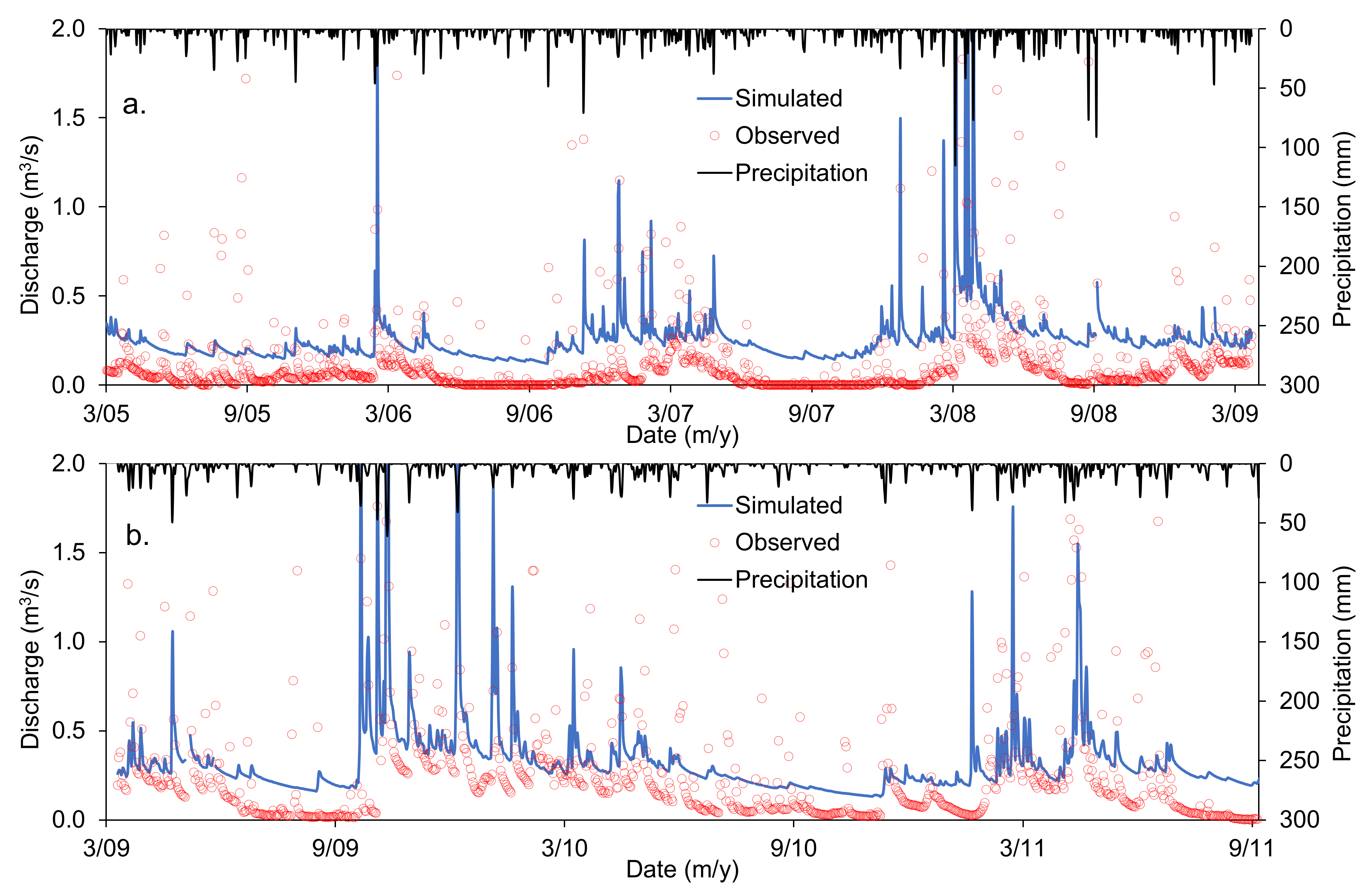
The R, MAE, BIAS, and NSE for the observed and measured surface water at the SW-GC gage station were 0.80, 0.20 m3/s, −0.14 m3/s, and 0.51, respectively (Figure 3a and Table 2). Unlike for groundwater, negative BIAS (−0.14 m3/s) showed that MIKE SHE overpredicted surface water flow during the calibration period. The surface water flow prediction during the validation period at the SW-GC gage station was R, 0.65, 0.22 m3/s, −0.02 m3/s, and 0.42 for MAE, BIAS, and NSE, respectively (Figure 3b and Table 2).

3.1.2. NOAA-Edwardsville Vs NOAA-St. Louis

The weighted average MAEs for groundwater elevations were 0.09 m (0.07 m to 0.11 m) and 0.15 m (0.03 to 0.21 m) for NOAA-Edwardsville and NOAA-St. Louis models, respectively at all four GW stations. The values reported in parenthesis are a range. Similarly, weighted average R were 0.78 (0.73 to 0.82) and 0.65 (0.58 to 0.70) for NOAA-Edwardsville and NOAA-St. Louis precipitation models, respectively (Table 3). The results showed that the NOAA-Edwardsville model performed better (values close to the CFSR model) than for NOAA-St. Louis considering average R and MAE.
The weighted average MAE for surface water flows for the NOAA-Edwardsville and NOAA-St. Louis models were 0.78 m3/s (0.02 to 1.02 m3/s) and 0.68 m3/s (0.02 to 0.91 m3/s), respectively (Table 3). Similarly, weighted average R were 0.64 (0.62 to 0.66) and 0.41 (0.34 to 0.46) for the NOAA-Edwardsville and NOAA-St. Louis models, respectively. The results showed NOAA-St. Louis model performed better (close to the CFSR model) than for the NOAA-Edwardsville considering average MAE, whereas the trend was opposite for R.

3.2. Effect of Precipitation on Groundwater and Surface Water Flows

3.2.1. Sensitive Variable (i.e., Groundwater Elevations or Surface Water Flows)

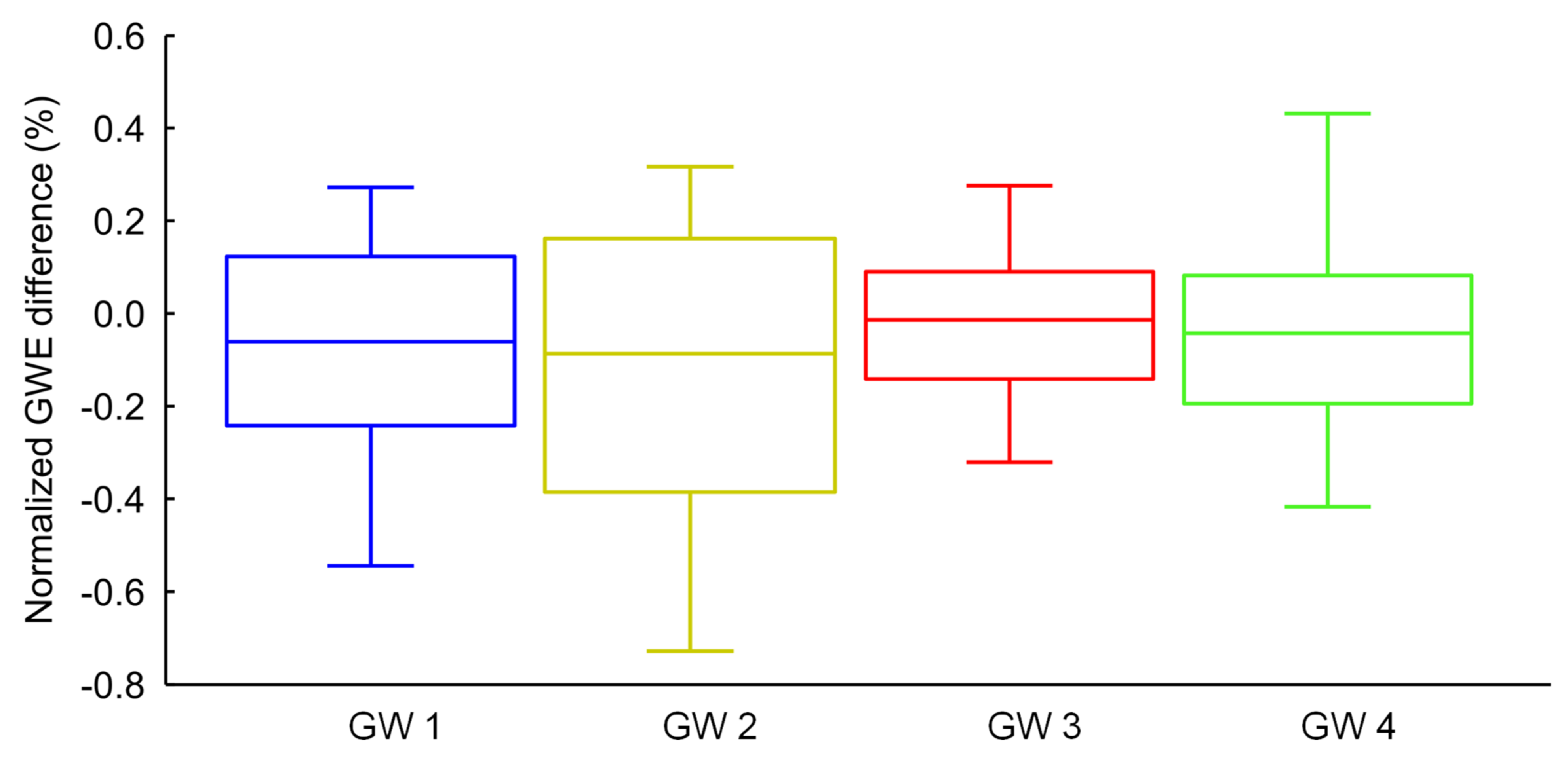
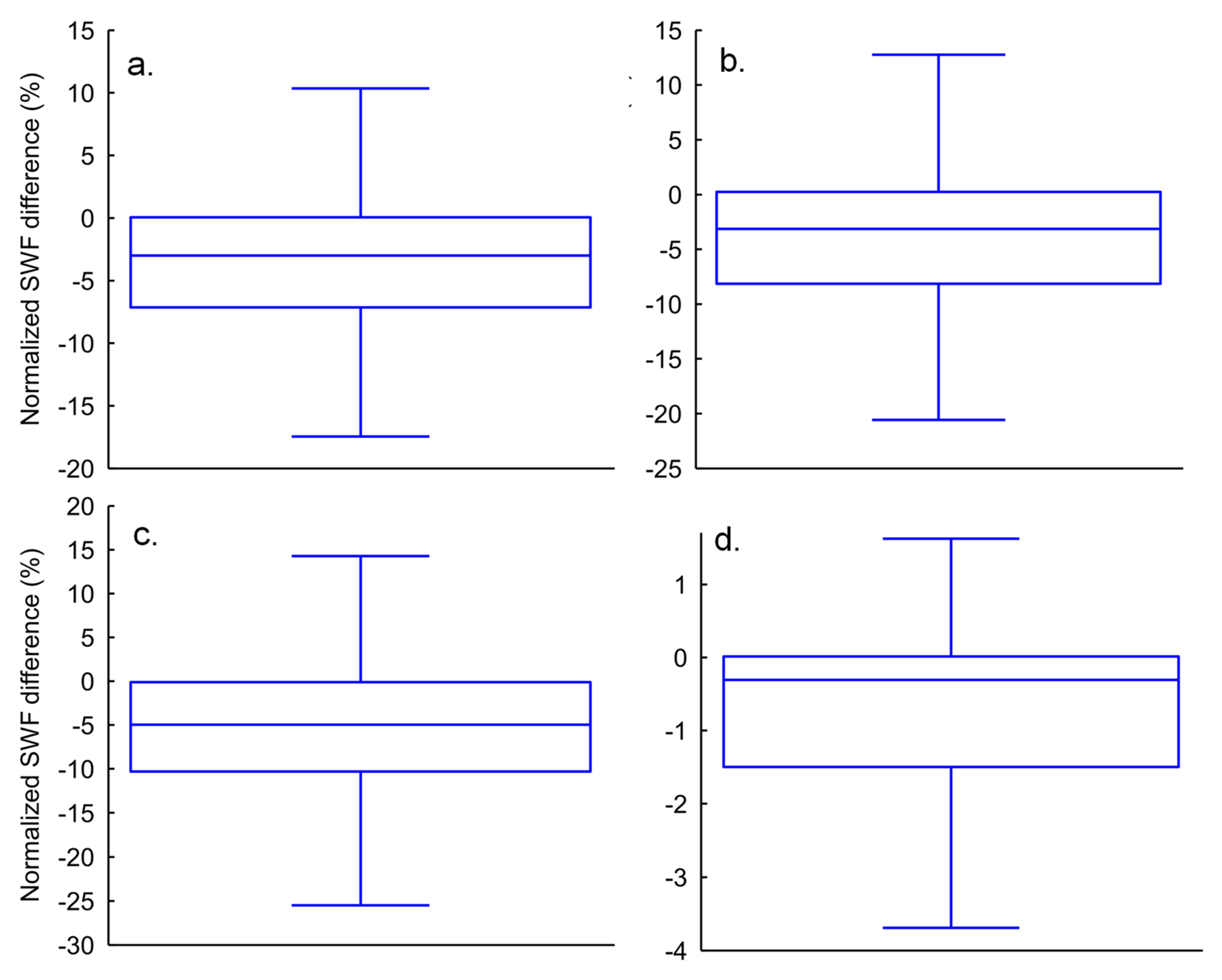
The weighted average MAE (considering all four stations) for simulated groundwater elevations and surface water flows were 0.07% (0.06% to 0.08%) and 6.71% (0.81% to 11.19%) for NOAA-Edwardsville and NOAA-St. Louis models, respectively (Table 4). Similarly, the average R were 0.78 (0.73 to 0.82) and 0.66 (0.63 to 0.72) for simulated groundwater elevations and surface water flows, respectively (Table 4). Therefore, differences were higher for surface water flows considering both MAE and R. Nevertheless, differences in daily average groundwater and surface water flow between NOAA-Edwardsville and NOAA-St. Louis models vary at each station (Figure 4 and Figure 5). For example, the difference in surface water flows varied from −18% to 10% at station 1, whereas −4% to 1% at station 4 (Figure 5). Negative values indicated higher surface water flows or groundwater elevations for the NOAA-Edwardsville model.

3.2.2. Seasonal Variations of Difference in Surface Water Flow with Respect to Change in Precipitation

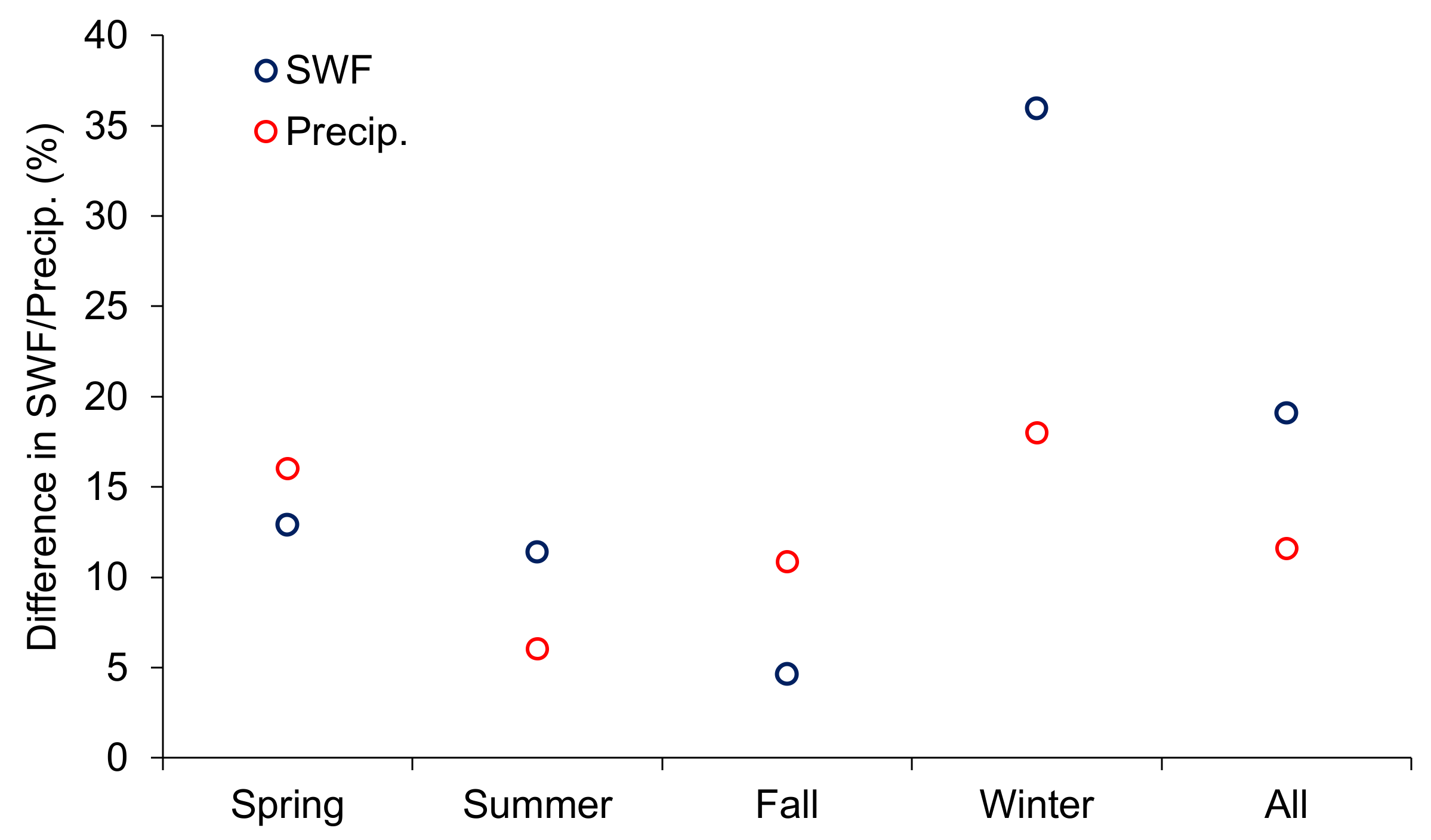
Considering all (April 2005 to April 2007) datasets, the difference in precipitation between NOAA-Edwardsville and NOAA-St. Louis gauge was 12.6%, whereas the difference in surface water flows was 19% (Figure 6). Seasonal differences in precipitation varied between 6% (summer) to 18% (winter), which resulted in the difference in surface water flow between 4.6% (fall) to 36% (winter) (Figure 6). The difference in surface water flows was relatively lower in fall (4.6%) and summer (11.4%) compared to spring (12.9%) and winter (36%). The highest difference for surface water flows was in the winter (36%) between NOAA-Edwardsville and NOAA-St. Louis models.

4. Discussion

4.1. Model Performance

We estimated the model performance statistical indicators R, MAE, BIAS, and NSE to analyze model performance against measured groundwater elevations and surface water flows at USGS gauge stations (Figure 1) [75,76]. We observed mixed model performance based on different statistical model performance indicators. The model performed satisfactorily considering MAE, where the values were generally less than half of SD (standard deviation) of observed flows [76] (Table 2). The model performance was comparable to past studies considering statistical model performance indicators [77,78]. The model performance was similar during calibration and validation periods (Table 2). In general, the model overpredicted baseflow during non-rainfall events for both calibration and validation periods (Figure 3). Nonetheless, based on the criteria suggested by prior researchers for model performance interpretation, the model performance for a small watershed is deemed satisfactory [67,75,76].
The model performances were analyzed by removing the days when the measured precipitation at CFSR and NOAA-Edwardsville gauge stations differed considerably during calibration and validation periods. Based on our judgement, precipitation measurements had uncertainties (either in CFSR or NOAA-Edwardsville gauges) during those days. We removed 34 (2.3%) and 12 (1.3%) data points out of 1461 and 913, respectively during the calibration and validation processes. Therefore, care should be taken while interpreting the model performance. It is a common practice to remove poorly performing datasets during hydrological model results analyses, however, it may change statistics and data distribution (e.g., mean, SD and range) [79,80,81,82].
Furthermore, we calculated the correlation between the measured precipitation (CFSR) and surface water flows at a USGS SW-GC gauge station (April 2005 to March 2012), which was relatively low (R = 0.53) (Figure 7a). The differences were evident during high precipitation and flow events. The lack of good correlations between measured surface flows and precipitations as well extreme events may cause poor model performance.
This study used CFSR based precipitation for model calibration, which was interpolated on a 38 km grid [35]. Various studies have shown that spatially distributed rainfall at a fine resolution is required for small scales analyses [40,83]. For example, 2 km grid rainfall was suggested by Bell and Moore [41] to model a small watershed (i.e., 132 km2 in size).
A small watershed may have a steep flow slope (flow change faster), high flow variations, and flashy hydrographs compared to a moderate and large watershed that may cause unsatisfactory model performance [46]. Runoff estimation improves as the watershed size increases, despite low rainfall resolution data [40,84]. Cunha, Mandapaka, Krajewski, Mantilla and Bradley [31] investigated the impact of the radar-rainfall error on hydrological model simulated flood magnitude and concluded that uncertainties in simulated peak flow decrease considerably with larger watersheds. Furthermore, as the watershed area increases, the peak flow differences at outlets were practically negligible. The measured surface water flows at the USGS gauge station were comparatively variable (flashy) than measured precipitation in this study, which is a typical trend for a small watershed (Figure 3 and Figure 7a). Furthermore, another study showed that the calibration performance of the model was distinct for two different precipitation datasets (gauge station and NEXRAD). The NEXRAD data performed better than the gauge station for a small watershed [28]. Therefore, we speculated that the model performance was affected by a small drainage area (21.3 km2 at the USGS gauge station) and limited observed data (single gauge station for groundwater and surface water measurements) availability in this study. The GW-GC station had 20 and 11 groundwater elevations measurements during the calibration and validation periods, respectively. Additionally, GW-PB (Figure 1) has only a total of seven data points, which were used to further verify the model performance for groundwater elevation predictions [85].
The time step and the grid size used in the model can affect the model performances [86,87,88]. A daily time step was used in this study, but Zhang, Wang, Sun, McNulty, Zhang, Li, Zhang, Klaghofer and Strauss [67] suggested that the daily (24 hours) time step may not be sufficient to capture a quick response of precipitation on surface runoff in overland flow dominant watersheds. The model was not able to predict highly variable surface water flows at the USGS gauge station as a result of rainfall. Specifically, during high events, peak flows occur within a few hours (less than 24 hours model time step) in the Canteen-Cahokia watershed, which comprises low stream lengths and channels [89].
Evapotranspiration (ET) had significant effects on groundwater and surface water flows [90]. A total of nine different land-use types (developed land, cultivated crops, bare soil, deciduous forest, evergreen forest, hay/pasture, woody wetlands, open water, and herbaceous wetlands) were considered in the analysis. An inaccurate representation of land-use impacts surface runoff, soil moisture, and groundwater recharge spatially and temporally in a distributed hydrological model [9,65,91,92]. Furthermore, because of lack of sufficient vegetation parameters (i.e., LAI and RD), temporal vegetation distribution was assumed to be constant and such a generalization can impact the model performance [93].
Despite some uncertainties in the model, we deemed that the model performance is acceptable to analyze the effects of precipitation on groundwater and surface water flows in a small watershed. Although the calibrated model (with CFSR precipitation) had certain uncertainties in model parameters, it was consistent across all three models. Therefore, the model should not noticeably distort the outcome when comparing the effects of different types of precipitation on hydrological processes.
Precipitation has the most critical influence on hydrological processes [28,39]; therefore, quality data is warranted for better model performance. The lack of finer spatial resolution of precipitation, and a high level of sensitivity of precipitation on a smaller spatial scale watershed influences the performance of the hydrological model [28]. Despite NOAA gauge network and radar-based precipitation being available for larger areas and different temporal resolutions (e.g., daily), uncertainties remained, which effect simulated hydrological processes [31,39]. Therefore, our results showed the importance of spatially and temporally varied high-resolution precipitation and surface water flow measurements for better model performance in small watersheds specifically to simulate surface water flows. The model performance is also affected by uncertainties in other datasets such as meteorological, land-use, soil type, topography, observed surface water flows and groundwater elevations, and scale (size) of the watershed [16,30,49].
Nonetheless, each of the models can be calibrated using NOAA meteorological and precipitation data. In that case, the effects of precipitation on groundwater elevations and surface water flows may have been different [35]. However, there is a fundamental issue with calibrating the model with different datasets and comparing the results. For example, calibrations using the two data sources may result in different model parameterizations, although having the same watershed characteristics. This may cause parameters overly influential in model results, which is also known as an equifinality [15,39].
We did not find a consistent pattern that the nearer gauge (i.e., NOAA-Edwardsville) station precipitation model performance is better (close to the CFSR model) than the farther gauge (i. e., NOAA-St. Louis) considering different statistical model performance indicators (MAE and R) for groundwater elevations and surface water flows at individual random stations (Table 3). However, Radcliffe and Mukundan [35], found better results from the model that has precipitation measured at a nearer gauge station than for the farther one.
CFSR Vs NOAA-Edwardsville (R = 0.31) measured precipitation had a higher correlation than for CFSR Vs NOAA-St. Louis (0.005) (Figure 7b,c). Our results showed a similar pattern (NOAA-Edwardsville performing better) for simulated groundwater elevations and surface water considering R (Table 3). However, NOAA-St. Louis model had a lower average MAE than for the NOAA-Edwardsville, despite NOAA-Edwardsville average precipitation being closer to the CFSR. The average ± SD (standard deviation) precipitation (April 2005 to January 2007) at CFSR, NOAA-Edwardsville, and NOAA-St. Louis gauge stations were 2.43 ± 6.34 mm, 2.46 ± 7.33 mm, and 2.17 ± 6.72 mm, respectively. Nevertheless, we just considered two gauge stations located around the watershed, but need to analyze results based on multiple gauges farther apart spatially before drawing any concrete conclusion regarding the model performance based on spatial distances of gauge stations.

4.2. Effects of Precipitation on Groundwater and Surface Water

An analysis of the most sensitive variable (groundwater elevation or surface water flow) showed that the effect of precipitation is more considerable in surface water flows (0.81% to 11.19%), than groundwater elevations (0.06% to 0.08%) (Table 4). Effects vary noticeably considering individual stations and daily average flows and groundwater elevations (Figure 4 and Figure 5). Although past studies have shown contradicting results regarding the relationship between precipitation and groundwater elevations [50,51,52], our results showed minimal (0.06% to 0.08%) effects of precipitation on simulated groundwater elevations. Our results are consistent with Gardner and Heilweil [94], where they concluded groundwater elevations respond slowly to precipitation.
Our study did not show a systematic change in surface water flows as a result of the difference in precipitation (Figure 6) but they were season-specific. We found the lowest difference in surface water flows in summer and fall seasons, which might be due to a higher evapotranspiration rate resulting in lower flows in rivers [95]. Evapotranspiration increases with higher atmospheric temperature and impacts surface runoff balance in river systems. The difference in surface water flow change depends on precipitation, atmospheric temperature, evapotranspiration as well as groundwater contributions [50,51,52,53], which support our results. Surface water flows changes were relatively less in summer and fall seasons despite higher differences in precipitation (Figure 6) because of higher evapotranspiration from the system [95]. Decreasing trends in baseflow within the US Midwest are attributed to increasing temperatures and evapotranspiration during the summer months [53].

4.3. Study Application

Our study has shown that care should be taken while selecting input datasets (e.g., precipitation) for hydrological model development and forecasting hydrological processes [16,39]. Many important factors should be considered before selecting precipitation data sources for simulating groundwater elevations and surface water flows, for example, the spatial and temporal scale of the model, rain gauge data availability, watershed area, input data quality, and model structure and spatial discretization [28]. Based on our results, the effects of precipitation uncertainties on simulated surface water flows vary season by season because of changing atmospheric temperature and evapotranspiration processes [95]. Our results suggested that high temporal and spatial resolution input data and the data used for model calibration (groundwater elevation and surface water flows) would improve hydrological model performance to simulate surface water flows than for groundwater elevations. The results emphasized the importance of the accurate input datasets (e.g., precipitation) for reliable model predictions [39,48]. The model developed in this study can be used to simulate hydrological processes in the future for the Canteen–Cahokia watershed to analyze impacts on future climate change and land cover changes due to urbanization on the hydrological process (groundwater elevations and surface water flows), and subsequent impacts on ecosystems (aquatic and riparian) and urban flooding [96,97]. This study is focused on a small watershed; therefore, further studies are required to transfer the findings to other watersheds in different geographic regions and large watersheds.

5. Conclusions

A spatially distributed MIKE SHE integrated hydrological model was calibrated and validated with daily averaged measured groundwater elevations and surface water flows. The calibrated model was used to analyze the effects of different precipitation on simulated hydrologic processes (i.e., groundwater elevations and surface water flows). The MIKE SHE model was able to predict surface water flows and groundwater elevations with reasonable accuracy at daily time steps for a small watershed. The study did not conclusively show that the model based on precipitation measured at nearer gauge (NOAA-Edwardsville) performs better than the model based on farther gauge (NOAA-St. Louis) precipitation.
The analyses for the most sensitive model output variable showed that differences in precipitation had noticeable (0.81% to 11.19%) effect on simulated surface water flows, whereas it had minimal (0.06% to 0.08%) effects on groundwater elevations. We found greater differences in simulated surface water flows in spring (12.9%) and winter (36%) compared to summer (11.4%) and fall (4.6%) due to difference in precipitations (6% to 18%) measured at NOAA-Edwardsville and NOAA-St. Louis gauges. The study showed that uncertainties in precipitation on simulated surface water flows vary with the season in a small watershed.

Author Contributions

Conceptualization, R.B.; Data curation, S.P.; Formal analysis, S.P.; Funding acquisition, R.B.; Investigation, R.B.; Methodology, S.P. and R.B.; Software, S.P.; Supervision, R.B.; Validation, S.P.; Writing—original draft, S.P. and R.B.; Writing—review & editing, S.P. and R.B. All authors have read and agreed to the published version of the manuscript.

Funding

This research received no external funding.

Data Availability Statement

Please contact corresponding author for data.

Acknowledgments

We acknowledge Danish Hydraulic Institute (DHI) for providing MIKE SHE and MIKE Hydro software for the study. We would like to thank SIUE Undergraduate Research and Creative Activities (URCA) student, Abin Paudel for helping to analyze NOAA precipitation data. The comments from the reviewers’ earlier versions helped us to improve the manuscript significantly. Sabin Paudel is funded through SIUE Civil Engineering Department and Graduate School during his study period. We also acknowledge Ryan Fries and Yan Qi for constructive comments in an earlier version of the manuscript.

Conflicts of Interest

The authors declare no conflict of interest.

References

  1. Gordon, L.J.; Finlayson, C.M.; Falkenmark, M. Managing water in agriculture for food production and other ecosystem services. Agric. Water Manag. 2010, 97, 512–519. [Google Scholar] [CrossRef]
  2. Ma, C.; Zhang, G.Y.; Zhang, X.C.; Zhou, B.; Jiang, W.X. Water resource management for wetland restoration engineering in Tianjin coastal area in China. Adv. Mater. Res. 2012, 518, 4333–4336. [Google Scholar] [CrossRef]
  3. Benjankar, R.; Jorde, K.; Yager, E.M.; Egger, G.; Goodwin, P.; Glenn, N.F. The Impact of River Modification and Dam Operation on Floodplain Vegetation Succession Trends in the Kootenai River, USA. Ecol. Eng. 2012, 46, 88–97. [Google Scholar] [CrossRef]
  4. Benjankar, R.; Tranmer, A.W.; Vidergar, D.; Tonina, D. Riparian vegetation model to predict seedling recruitment and restoration alternatives. J. Environ. Manag. 2020, 276, 111339. [Google Scholar] [CrossRef]
  5. Dai, Z.; Li, C.; Trettin, C.; Sun, G.; Amatya, D.; Li, H. Bi-criteria evaluation of the MIKE SHE model for a forested watershed on the South Carolina coastal plain. Hydrol. Earth Syst. Sci. 2010, 14, 1033–1046. [Google Scholar] [CrossRef] [Green Version]
  6. Ruelland, D.; Ardoin-Bardin, S.; Billen, G.; Servat, E. Sensitivity of a lumped and semi-distributed hydrological model to several methods of rainfall interpolation on a large basin in West Africa. J. Hydrol. 2008, 361, 96–117. [Google Scholar] [CrossRef]
  7. Harbaugh, A.W. MODFLOW-2005: The US Geological Survey Modular Ground-Water Model: The Ground-Water Flow Process; US Geological Survey Reston: Reston, VA, USA, 2005. [Google Scholar]
  8. Sahoo, G.; Ray, C.; De Carlo, E. Calibration and validation of a physically distributed hydrological model, MIKE SHE, to predict streamflow at high frequency in a flashy mountainous Hawaii stream. J. Hydrol. 2006, 327, 94–109. [Google Scholar] [CrossRef]
  9. Graham, D.N.; Butts, M.B. Flexible, integrated watershed modelling with MIKE SHE. Watershed Models 2005, 849336090, 245–272. [Google Scholar]
  10. Doummar, J.; Sauter, M.; Geyer, T. Simulation of flow processes in a large scale karst system with an integrated catchment model (Mike She)—Identification of relevant parameters influencing spring discharge. J. Hydrol. 2012, 426, 112–123. [Google Scholar] [CrossRef]
  11. Madsen, H.; Jacobsen, T. Automatic calibration of the MIKE SHE integrated hydrological modelling system. In Proceedings of the 4th DHI Software Conference, Helsingor, Denmark, 6–8 June 2001; pp. 6–8. [Google Scholar]
  12. Refsgaard, J.C. Parameterisation, calibration and validation of distributed hydrological models. J. Hydrol. 1997, 198, 69–97. [Google Scholar] [CrossRef]
  13. Oogathoo, S. Runoff Simulation in the Canagagigue Creek Watershed using the MIKE SHE Model. Master’s Thesis, McGill University, Montreal, QC, Canada, August 2006. [Google Scholar]
  14. Arnold, J.; Allen, P.; Volk, M.; Williams, J.; Bosch, D. Assessment of different representations of spatial variability on SWAT model performance. Trans. ASABE 2010, 53, 1433–1443. [Google Scholar] [CrossRef]
  15. Price, K.; Purucker, S.T.; Kraemer, S.R.; Babendreier, J.E.; Knightes, C.D. Comparison of radar and gauge precipitation data in watershed models across varying spatial and temporal scales. Hydrol. Process. 2014, 28, 3505–3520. [Google Scholar] [CrossRef]
  16. Fu, S.; Sonnenborg, T.O.; Jensen, K.H.; He, X. Impact of precipitation spatial resolution on the hydrological response of an integrated distributed water resources model. Vadose Zone J. 2011, 10, 25–36. [Google Scholar] [CrossRef]
  17. Vischel, T.; Lebel, T. Assessing the water balance in the Sahel: Impact of small scale rainfall variability on runoff. Part 2: Idealized modeling of runoff sensitivity. J. Hydrol. 2007, 333, 340–355. [Google Scholar] [CrossRef]
  18. Strauch, M.; Bernhofer, C.; Koide, S.; Volk, M.; Lorz, C.; Makeschin, F. Using precipitation data ensemble for uncertainty analysis in SWAT streamflow simulation. J. Hydrol. 2012, 414, 413–424. [Google Scholar] [CrossRef]
  19. Zhang, W.; Montgomery, D.R. Digital elevation model grid size, landscape representation, and hydrologic simulations. Water Resour. Res. 1994, 30, 1019–1028. [Google Scholar] [CrossRef]
  20. Smith, M.B.; Koren, V.I.; Zhang, Z.; Reed, S.M.; Pan, J.-J.; Moreda, F. Runoff response to spatial variability in precipitation: An analysis of observed data. J. Hydrol. 2004, 298, 267–286. [Google Scholar] [CrossRef]
  21. Berne, A.; Delrieu, G.; Creutin, J.-D.; Obled, C. Temporal and spatial resolution of rainfall measurements required for urban hydrology. J. Hydrol. 2004, 299, 166–179. [Google Scholar] [CrossRef]
  22. McGregor, G.R.; Nieuwolt, S. Tropical Climatology: An Introduction to the Climates of the Low Latitudes; John Wiley & Sons Ltd.: Chichester, UK, 1998. [Google Scholar]
  23. Singh, P.; Kumar, N. Effect of orography on precipitation in the western Himalayan region. J. Hydrol. 1997, 199, 183–206. [Google Scholar] [CrossRef]
  24. Marino, P.; Comegna, L.; Damiano, E.; Olivares, L.; Greco, R. Monitoring the Hydrological Balance of a Landslide-Prone Slope Covered by Pyroclastic Deposits over Limestone Fractured Bedrock. Water 2020, 12, 3309. [Google Scholar] [CrossRef]
  25. Greco, R.; Comegna, L.; Damiano, E.; Marino, P.; Olivares, L.; Santonastaso, G.F. Recurrent rainfall-induced landslides on the slopes with pyroclastic cover of Partenio Mountains (Campania, Italy): Comparison of 1999 and 2019 events. Eng. Geol. 2021, 288, 106160. [Google Scholar] [CrossRef]
  26. Yeh, H.-F.; Lee, C.-H. Soil water balance model for precipitation-induced shallow landslides. Environ. Earth Sci. 2013, 70, 2691–2701. [Google Scholar] [CrossRef]
  27. Masih, I.; Maskey, S.; Uhlenbrook, S.; Smakhtin, V. Assessing the impact of areal precipitation input on streamflow simulations using the SWAT Model 1. JAWRA J. Am. Water Resour. Assoc. 2011, 47, 179–195. [Google Scholar] [CrossRef]
  28. Bredesen, A.; Brown, C. Comparison of Hydrologic Model Performance Statistics Using Rain Gauge and NEXRAD Precipitation Input at Different Watershed Spatial Scales and Rainfall Return Frequencies for the Upper St. Johns River, Florida USA. Proceedings 2018, 7, 11. [Google Scholar] [CrossRef] [Green Version]
  29. Smith, T.M.; Arkin, P.A.; Ren, L.; Shen, S.S. Improved reconstruction of global precipitation since 1900. J. Atmos. Ocean. Technol. 2012, 29, 1505–1517. [Google Scholar] [CrossRef]
  30. Yu, M.; Chen, X.; Li, L.; Bao, A.; De la Paix, M.J. Streamflow simulation by SWAT using different precipitation sources in large arid basins with scarce raingauges. Water Resour. Manag. 2011, 25, 2669. [Google Scholar] [CrossRef]
  31. Cunha, L.K.; Mandapaka, P.V.; Krajewski, W.F.; Mantilla, R.; Bradley, A.A. Impact of radar-rainfall error structure on estimated flood magnitude across scales: An investigation based on a parsimonious distributed hydrological model. Water Resour. Res. 2012, 48, 1–22. [Google Scholar] [CrossRef]
  32. Moon, J.; Srinivasan, R.; Jacobs, J. Stream flow estimation using spatially distributed rainfall in the Trinity River basin, Texas. Trans. ASAE 2004, 47, 1445. [Google Scholar] [CrossRef]
  33. Obled, C.; Wendling, J.; Beven, K. The sensitivity of hydrological models to spatial rainfall patterns: An evaluation using observed data. J. Hydrol. 1994, 159, 305–333. [Google Scholar] [CrossRef]
  34. Bárdossy, A.; Das, T. Influence of rainfall observation network on model calibration and application. Hydrol. Earth Syst. Sci. 2008, 12, 77–89. [Google Scholar] [CrossRef] [Green Version]
  35. Radcliffe, D.; Mukundan, R. PRISM vs. CFSR precipitation data effects on calibration and validation of SWAT models. JAWRA J. Am. Water Resour. Assoc. 2017, 53, 89–100. [Google Scholar] [CrossRef]
  36. Molini, A.; Lanza, L.; La Barbera, P. The impact of tipping-bucket raingauge measurement errors on design rainfall for urban-scale applications. Hydrol. Process. Int. J. 2005, 19, 1073–1088. [Google Scholar] [CrossRef]
  37. Groisman, P.Y.; Legates, D.R. The accuracy of United States precipitation data. Bull. Am. Meteorol. Soc. 1994, 75, 215–228. [Google Scholar] [CrossRef]
  38. Krajewski, W.; Smith, J.A. Radar hydrology: Rainfall estimation. Adv. Water Resour. 2002, 25, 1387–1394. [Google Scholar] [CrossRef]
  39. Sirisena, T.A.J.G.; Maskey, S.; Ranasinghe, R.; Babele, M.S. Effects of different precipitation inputs on streamflow simulation in the Irrawaddy River Basin, Myanmar. J. Hydrol. Reg. Stud. 2018, 19, 265–278. [Google Scholar] [CrossRef]
  40. Segond, M.-L.; Wheater, H.S.; Onof, C. The significance of spatial rainfall representation for flood runoff estimation: A numerical evaluation based on the Lee catchment, UK. J. Hydrol. 2007, 347, 116–131. [Google Scholar] [CrossRef]
  41. Bell, V.; Moore, R. The sensitivity of catchment runoff models to rainfall data at different spatial scales. Hydrol. Earth Syst. Sci. 2000, 4, 653–667. [Google Scholar] [CrossRef]
  42. Koren, V.; Finnerty, B.; Schaake, J.; Smith, M.; Seo, D.-J.; Duan, Q.-Y. Scale dependencies of hydrologic models to spatial variability of precipitation. J. Hydrol. 1999, 217, 285–302. [Google Scholar] [CrossRef]
  43. Fuka, D.; Walter, M.; MacAlister, C.; Degaetano, A.; Steenhuis, T.; Easton, Z. Using the climate forecast system reanalysis as weather input data for watershed models: Using CFSR as weather input data for watershed models. Hydrol. Process. 2014, 28, 5613–5623. [Google Scholar] [CrossRef]
  44. Najafi, M.R.; Moradkhani, H.; Piechota, T.C. Ensemble streamflow prediction: Climate signal weighting methods vs. climate forecast system reanalysis. J. Hydrol. 2012, 442–443, 105–116. [Google Scholar] [CrossRef]
  45. Smith, R.A.; Kummerow, C.D. A comparison of in situ, reanalysis, and satellite water budgets over the upper Colorado River basin. J. Hydrometeorol. 2013, 14, 888–905. [Google Scholar] [CrossRef]
  46. Goodarzi, M.; Amiri, B.J.; Azarneyvand, H.; Khazaee, M.; Mahdianzadeh, N. Assessing the performance of a hydrological tank model at various spatial scales. J. Water Manag. Modeling. 2020, 28, 1–8. [Google Scholar] [CrossRef]
  47. Lopes, V.L. On the effect of uncertainty in spatial distribution of rainfall on catchment modelling. Catena 1996, 28, 107–119. [Google Scholar] [CrossRef]
  48. Guo, J.; Liang, X.; Leung, L.R. Impacts of different precipitation data sources on water budgets. J. Hydrol. 2004, 298, 311–334. [Google Scholar] [CrossRef]
  49. Carpenter, T.M.; Georgakakos, K.P. Impacts of parametric and radar rainfall uncertainty on the ensemble streamflow simulations of a distributed hydrologic model. J. Hydrol. 2004, 298, 202–221. [Google Scholar] [CrossRef]
  50. Vitola, I.; Vircavs, V.; Abramenko, K.; Lauva, D.; Veinbergs, A. Precipitation and Air Temperature Impact on Seasonal Variations of Groundwater Levels. Environ. Clim. Technol. 2012, 10, 25–33. [Google Scholar] [CrossRef] [Green Version]
  51. Wu, W.-Y.; Lo, M.-H.; Wada, Y.; Famiglietti, J.S.; Reager, J.T.; Yeh, P.J.-F.; Ducharne, A.; Yang, Z.-L. Divergent effects of climate change on future groundwater availability in key mid-latitude aquifers. Nat. Commun. 2020, 11, 3710. [Google Scholar] [CrossRef]
  52. Haucke, J. Precipitation and Pumping Effects on Groundwater Levels in Central Wisconsin; University of Wisconsin: Stevens Point, WI, USA, 2010. [Google Scholar]
  53. Ayers, J.R.; Villarini, G.; Jones, C.; Schilling, K. Changes in monthly baseflow across the U.S. Midwest. Hydrol. Process. 2019, 33, 748–758. [Google Scholar] [CrossRef]
  54. Refsgaard, J.C.; Højberg, A.L.; Møller, I.; Hansen, M.; Søndergaard, V. Groundwater modeling in integrated water resources management—Visions for 2020. Groundwater 2010, 48, 633–648. [Google Scholar] [CrossRef]
  55. Danish Hydraulic Institute (DHI). MIKE SHE User Guide; DHI: Hørsholm, Denmark, 2017. [Google Scholar]
  56. Bogdanov, L.; Zakharov, V. The Boussinesq equation revisited. Phys. D Nonlinear Phenom. 2002, 165, 137–162. [Google Scholar] [CrossRef]
  57. Kristensen, K.; Jensen, S. A model for estimating actual evapotranspiration from potential evapotranspiration. Hydrol. Res. 1975, 6, 170–188. [Google Scholar] [CrossRef] [Green Version]
  58. Thompson, J.; Sørenson, H.R.; Gavin, H.; Refsgaard, A. Application of the coupled MIKE SHE/MIKE 11 modelling system to a lowland wet grassland in southeast England. J. Hydrol. 2004, 293, 151–179. [Google Scholar] [CrossRef]
  59. Gaur, S.; Bandyopadhyay, A.; Singh, R. Projecting land use growth and associated impacts on hydrological balance through scenario-based modelling in the Subarnarekha basin, India. Hydrol. Sci.J. 2021, 66, 1997–2010. [Google Scholar] [CrossRef]
  60. Refsgaard, J.C.; Storm, B. Computer Models of Watershed Hydrology; Singh, V.P., Ed.; Water Resource Publications, LLC: Littleton, CO, USA, 1995; pp. 809–846. [Google Scholar]
  61. Saha, S.; Moorthi, S.; Pan, H.-L.; Wu, X.; Wang, J.; Nadiga, S.; Tripp, P.; Kistler, R.; Woollen, J.; Behringer, D.; et al. The NCEP climate forecast system reanalysis. Am. Meteorol. Soc. 2010, 91, 1015–1058. [Google Scholar] [CrossRef]
  62. Synder, R.L.; Eching, S. Daily Reference Evapotranspiration Calculator User’s Guide for PMday.xls; University of California: Oakland, CA, USA, 2006. [Google Scholar]
  63. Schwarz, G.E.; Alexander, R. State Soil Geographic (STATSGO) Data Base for the Conterminous United States; Open-File Report; USGS: Reston, VA, USA, 1995.
  64. Van Genuchten, M.T. A closed-form equation for predicting the hydraulic conductivity of unsaturated soils. Soil Sci. Soc. Am. J. 1980, 44, 892–898. [Google Scholar] [CrossRef] [Green Version]
  65. Im, S.; Kim, H.; Kim, C.; Jang, C. Assessing the impacts of land use changes on watershed hydrology using MIKE SHE. Environ. Geol. 2009, 57, 231. [Google Scholar] [CrossRef]
  66. Moriasi, D.; Wilson, B.; Douglas-Mankin, K.; Arnold, J.; Gowda, P. Hydrologic and water quality models: Use, calibration, and validation. Trans. ASABE 2012, 55, 1241–1247. [Google Scholar] [CrossRef]
  67. Zhang, Z.; Wang, S.; Sun, G.; McNulty, S.G.; Zhang, H.; Li, J.; Zhang, M.; Klaghofer, E.; Strauss, P. Evaluation of the MIKE SHE model for application in the Loess Plateau, China 1. JAWRA J. Am. Water Resour. Assoc. 2008, 44, 1108–1120. [Google Scholar] [CrossRef]
  68. Liu, H.-L.; Chen, X.; Bao, A.-M.; Wang, L. Investigation of groundwater response to overland flow and topography using a coupled MIKE SHE/MIKE 11 modeling system for an arid watershed. J. Hydrol. 2007, 347, 448–459. [Google Scholar] [CrossRef]
  69. Ogden, F.L.; Julien, P.Y. Runoff model sensitivity to radar rainfall resolution. J. Hydrol. 1994, 158, 1–18. [Google Scholar] [CrossRef]
  70. Komma, J.; Reszler, C.; Blöschl, G.; Haiden, T. Ensemble prediction of floods—Catchment non-linearity and forecast probabilities. Nat. Hazards Earth Syst. Sci. 2007, 7, 431–444. [Google Scholar] [CrossRef] [Green Version]
  71. Gupta, H.V.; Sorooshian, S.; Yapo, P.O. Status of automatic calibration for hydrologic models: Comparison with multilevel expert calibration. J. Hydrol. Eng. 1999, 4, 135–143. [Google Scholar] [CrossRef]
  72. Ritter, A.; Muñoz-Carpena, R. Performance evaluation of hydrological models: Statistical significance for reducing subjectivity in goodness-of-fit assessments. J. Hydrol. 2013, 480, 33–45. [Google Scholar] [CrossRef]
  73. Krause, P.; Boyle, D.; Bäse, F. Comparison of different efficiency criteria for hydrological model assessment. Adv. Geosci. 2005, 5, 89–97. [Google Scholar] [CrossRef] [Green Version]
  74. Willmott, C.J.; Matsuura, K. Advantages of the mean absolute error (MAE) over the root mean square error (RMSE) in assessing average model performance. Clim. Res. 2005, 30, 79–82. [Google Scholar] [CrossRef]
  75. Moriasi, D.N.; Gitau, M.W.; Pai, N.; Daggupati, P. Hydrologic and water quality models: Performance measures and evaluation criteria. Trans. ASABE 2015, 58, 1763–1785. [Google Scholar]
  76. Singh, J. Hydrologic Model of the Vermilion River Watershed for Streamflow Simulations; Illinois Department of Natural Resources and the Illinois State Geological Survey: Champaign, IL, USA, 2004.
  77. Sultana, Z.; Coulibaly, P. Distributed modelling of future changes in hydrological processes of Spencer Creek watershed. Hydrol. Process. 2011, 25, 1254–1270. [Google Scholar] [CrossRef]
  78. Qiu, L.-J.; Zheng, F.-L.; Yin, R.-S. SWAT-based runoff and sediment simulation in a small watershed, the loessial hilly-gullied region of China: Capabilities and challenges. Int. J. Sediment Res. 2012, 27, 226–234. [Google Scholar] [CrossRef]
  79. Krysanova, V.; Donnelly, C.; Gelfan, A.; Gerten, D.; Arheimer, B.; Hattermann, F.; Kundzewicz, Z.W. How the performance of hydrological models relates to credibility of projections under climate change. Hydrol. Sci. J. 2018, 63, 696–720. [Google Scholar] [CrossRef]
  80. Crochemore, L.; Isberg, K.; Pimentel, R.; Pineda, L.; Hasan, A.; Arheimer, B. Lessons learnt from checking the quality of openly accessible river flow data worldwide. Hydrol. Sci. J. 2020, 65, 699–711. [Google Scholar] [CrossRef] [Green Version]
  81. Pullen-Sansfaçon, A.; Spolander, G.; Engelbrecht, L. Migration of professional social workers: Reflections on challenges and strategies for education. Soc. Work. Educ. 2012, 31, 1032–1045. [Google Scholar] [CrossRef] [Green Version]
  82. Boughton, W. Calibrations of a daily rainfall-runoff model with poor quality data. Environ. Model. Softw. 2006, 21, 1114–1128. [Google Scholar] [CrossRef]
  83. Carpenter, T.M.; Georgakakos, K.P. Assessment of Folsom lake response to historical and potential future climate scenarios: 1. Forecasting. J. Hydrol. 2001, 249, 148–175. [Google Scholar] [CrossRef]
  84. Bulygina, N.; McIntyre, N.; Wheater, H. A comparison of rainfall-runoff modelling approaches forestimating impacts of rural land management onfloodflows. Hydrol. Res. 2013, 44, 467–483. [Google Scholar] [CrossRef]
  85. Paudel, S. Impact of Precipitation Sources on Surface Water and Groundwater Hydrology in Canteen-Cahokia Watershed, IL, USA; Southern Illinois University Edwardsville: Edwardsville, IL, USA, 2021. [Google Scholar]
  86. Vázquez, R.; Feyen, L.; Feyen, J.; Refsgaard, J. Effect of grid size on effective parameters and model performance of the MIKE-SHE code. Hydrol. Process. 2002, 16, 355–372. [Google Scholar] [CrossRef]
  87. Sohrabi, M.M.; Tonina, D.; Benjankar, R.; Kumar, M.; Kormos, P.; Marks, D. Role of temporal resolution of meteorological inputs for process-based snow modelling. Hydrol. Process. 2018, 32, 2976–2989. [Google Scholar] [CrossRef]
  88. Sohrabi, M.M.; Tonina, D.; Benjankar, R.; Kumar, M.; Kormos, P.; Marks, D.; Luce, C. On the role of spatial resolution on snow estimates using a process-based snow model across a range of climatology and elevation. Hydrol. Process. 2019, 33, 1260–1275. [Google Scholar] [CrossRef]
  89. United States Department of Agriculture (USDA). Urban Hydrology for Small Watersheds; United States Department of Agriculture (USDA): Washington, DC, USA, 1986; pp. 1–164.
  90. Célleri, R.; Timbe, L.; Vázquez, R.; Feyen, J. Assessment of the relation between the NAM rainfall-runoff model parameters and the physical catchment properties. HIP-VI UNESCO Tech. Doc. Hydrol. 2003, 66, 9–16. [Google Scholar]
  91. Singh, R.; Subramanian, K.; Refsgaard, J. Hydrological modelling of a small watershed using MIKE SHE for irrigation planning. Agric. Water Manag. 1999, 41, 149–166. [Google Scholar] [CrossRef]
  92. Tasser, E.; Mader, M.; Tappeiner, U. Effects of land use in alpine grasslands on the probability of landslides. Basic Appl. Ecol. 2003, 4, 271–280. [Google Scholar] [CrossRef]
  93. Christiaens, K.; Feyen, J. Analysis of uncertainties associated with different methods to determine soil hydraulic properties and their propagation in the distributed hydrological MIKE SHE model. J. Hydrol. 2001, 246, 63–81. [Google Scholar] [CrossRef]
  94. Gardner, P.M.; Heilweil, V.M. Evaluation of the Effects of Precipitation on Ground-Water Levels from Wells in Selected Alluvial Aquifers in Utah and Arizona, 1936–2005 U.S.; Geological Survey Scientific Investigations Report 2008-5242; USGS: Reston, VA, USA, 2009; p. 38.
  95. Garbrecht, J.; Liew, M.V.; Brown, G.O. Trends in Precipitation, Streamflow, and Evapotranspiration in the Great Plains of the United States. J. Hydrol. Eng. 2004, 9, 360–367. [Google Scholar] [CrossRef] [Green Version]
  96. Benjankar, R.; Tonina, D.; McKean, J.A.; Sohrabi, M.M.; Chen, Q.; Vidergar, D. An ecohydraulics virtual watershed: Integrating physical and biological variables to quantify aquatic habitat quality. Ecohydrology 2019, 12, e2062. [Google Scholar] [CrossRef]
  97. Benjankar, R.; Tonina, D.; Mckean, J.A.; Sohrabi, M.M.; Chen, Q.; Vidergar, D. Dam operations may improve aquatic habitat and offset negative effects of climate change. J. Environ. Manag. 2018, 213, 126–134. [Google Scholar] [CrossRef]
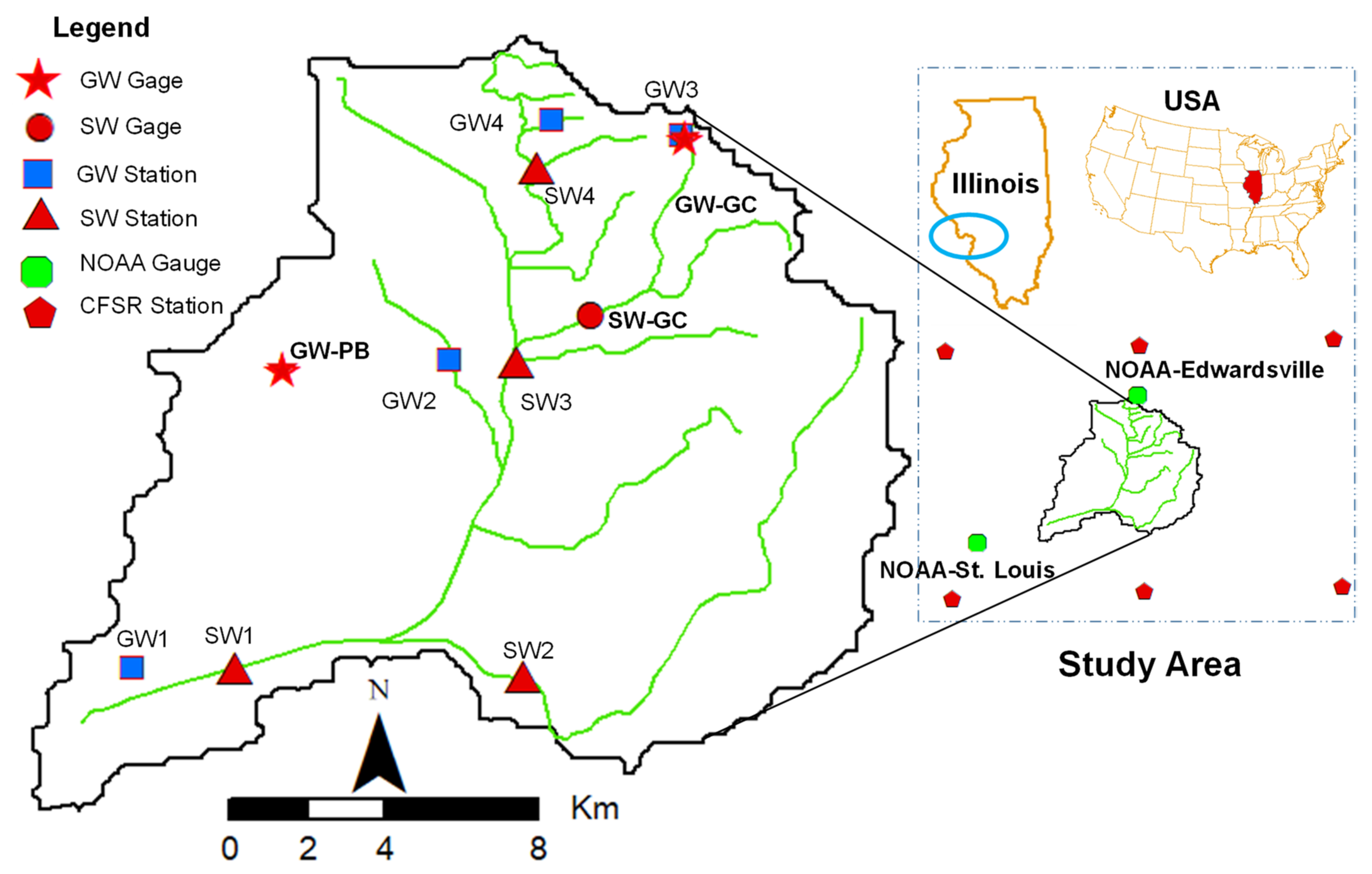
Figure 1. Location of Canteen-Cahokia watershed showing National Oceanic and Atmospheric Administration (NOAA) precipitation gauges, Climate Forecast System Reanalysis (CFSR) stations, and USGS groundwater (GW-GC: USGS Groundwater Station# 384656089582001 at Glen Carbon, Illinois) and surface water gauge stations (SW-GC: USGS surface water flow station# 05588720 at Glen Carbon, Illinois). SW = surface water, GW = groundwater, GC = Glen Carbon, PB = Pontoon Beach.
Hydrology 09 00037 g001
Figure 2. Measured and simulated daily groundwater elevations for (a) Calibration and (b) Validation periods at GW-GC gage station (USGS Groundwater Station# 384656089582001 at the city of Glen Carbon, IL).
Hydrology 09 00037 g002
Figure 3. Measured and simulated daily surface flow hydrograph at SW-GC gage (USGS surface water station# 05588720 at the city of Glen Carbon, IL) and CFSR precipitation depths for (a) Calibration and (b) Validation.
Hydrology 09 00037 g003
Figure 4. Distribution of difference (%) in simulated daily groundwater elevations at four different stations for NOAA-Edwardsville and NOAA-St. Louis models.
Hydrology 09 00037 g004
Figure 5. Distribution of difference in simulated daily surface water flows at four different stations from NOAA-Edwardsville and NOAA-St. Louis models. (a) Station 1; (b) Station 2; (c) Station 3; (d) Station 4.
Hydrology 09 00037 g005
Figure 6. Difference in precipitation (Precip.) and surface water flows (SWF) considering all (April 2005 to January 2007) and seasonal datasets based on NOAA-Edwardsville and NOAA-St. Louis models.
Hydrology 09 00037 g006
Figure 7. Correlations between (a) CFSR based precipitation and surface water flow (USGS gauge station at Glen Carbon), (b) CFSR and NOAA-Edwardsville precipitation, and (c) CFSR and NOAA-St. Louis precipitation.
Hydrology 09 00037 g007
Table 1. Final Optimized Calibrated Parameters for Surface water and Groundwater.
ModelParametersInitialRangeCalibrated
MIKE SHEOverland and Unsaturated Zone
Manning’s M1710–4026.80
Detention Storage (mm)20–10 5.08
Bypass Constant0.260.15–0.9 0.27
Saturated Zone
Horizontal Hydraulic Conductivity (10−6 m/s)5.60.0056–566 96.80
Vertical Hydraulic Conductivity (10−6 m/s)0.5656.69.68
Specific Yield0.20.2–0.4 0.20
Initial Potential (−m)51–10 6.32
ET Parameters (Kristensen And Jensen)
Canopy Interception (mm)0.050.05–0.4 0.07
C10.20.05–0.4 0.34
C20.20.05–0.4 0.06
C3 (mm/day)205–406.95
Aroot (/m)0.30.05–0.4 0.31
MIKE HydroRiver and Lakes
Manning’s M3610–4018.45
Leakage Coefficient (10−6)5.60.0056–5662.30
Table 2. Model performance statistics for the model calibration and validation. GW, SW, and GC stand for Groundwater, surface water, and Glen Carbon, respectively.
ParametersCalibrationValidation
GW-GCSW-GCGW-GCSW-GC
R 0.740.800.740.65
MAE (m, m3/s)0.450.200.390.22
SD *0.650.440.530.57
BIAS (m, m3/s)0.08−0.14−0.24−0.02
NSE0.350.590.140.42
* Standard deviation of measurement.
Table 3. Difference in model performance statistics between NOAA-Edwardsville Vs CFSR and NOAA-St. Louis Vs CFSR precipitation models for groundwater elevations and surface water flows at four random stations.
Groundwater Elevation
NOAA-EdwardsvilleParametersGW1GW2GW3GW4Average
R0.800.730.780.820.78
MAE (m)0.090.090.110.070.09
NOAA-St. LouisR0.700.630.580.680.65
MAE (m)0.030.100.230.210.15
Surface Water
NOAA-EdwardsvilleParametersSW1SW2SW3SW4Average
R0.660.620.630.640.64
MAE (m3/s)1.020.380.020.030.78
NOAA-St. LouisR0.460.380.340.450.41
MAE (m3/s)0.910.310.020.020.68
Table 4. MAE (%) and R between NOAA-Edwardsville Vs NOAA-St. Louis models for groundwater elevations and surface water flows at four random stations. The difference MAE (%) is calculated relative to the NOAA-Edwardsville model.
ParametersGW/SW1GW/SW2GW/SW3GW/SW4Average
GroundwaterR0.800.730.780.820.78
MAE (m)0.070.060.080.060.07
Surface WaterR0.720.640.650.630.66
MAE (m3/s)5.229.610.8111.196.71
Publisher’s Note: MDPI stays neutral with regard to jurisdictional claims in published maps and institutional affiliations.