Next Article in Journal
Determining the Hydrological Behaviour of Catchment Based on Quantitative Morphometric Analysis in the Hard Rock Area of Nand Samand Catchment, Rajasthan, India
Previous Article in Journal
Weekly Monitoring and Forecasting of Hydropower Production Coupling Meteo-Hydrological Modeling with Ground and Satellite Data in the Italian Alps
 
 
Correction published on 25 August 2022, see Hydrology 2022, 9(9), 154.
Article

Similarities in Evolution of Aggregate Size Distributions during Successive Wetting and Drying Cycles of Heavy Textured Soils of Variable Clay Mineralogy

by
Victor A. Snyder
* and
Miguel A. Vázquez
Departament of Agroenvironmental Sciences, University of Puerto Rico Agricultural Experiment Station, 1193 Guayacán Street, San Juan, PR 00936, USA
*
Author to whom correspondence should be addressed.
Hydrology 2022, 9(2), 30; https://doi.org/10.3390/hydrology9020030
Submission received: 30 December 2021 / Revised: 3 February 2022 / Accepted: 5 February 2022 / Published: 9 February 2022 / Corrected: 25 August 2022
(This article belongs to the Section Soil and Hydrology)

Abstract

:
A phenomenon causing instability of soil structure and associated hydraulic properties in recently tilled soils is aggregate fragmentation induced by wetting and drying cycles. We analyzed data from three experiments in Puerto Rico, the UK and China measuring fragmentation and resulting evolution of aggregate size distributions during successive wetting and drying cycles in heavy textured soils. Aggregate distributions were represented as the cumulative fraction F of aggregates passing through successively larger sieve sizes X. To a good approximation, all distributions exhibited similarity in that the aggregate diameter X(F) corresponding to F in a given test distribution was always a characteristic multiple α ¯ of X(F) in a fixed reference distribution, where α ¯ for a distribution was calculated as its mean weight aggregate diameter (MWD) divided by the MWD of the reference distribution. In most cases, α ¯ for a given soil varied inversely with the square of the number of wetting and drying cycles. For different soils of similar initial aggregate sizes, α ¯ for a given wet–dry cycle decreased with increasing activity coefficient, reflecting the enhancing effect of soil shrink–swell potential on fragmentation. Results highlight usefulness of the van Bavel mean weight diameter as a natural scaling parameter for characterizing aggregate distributions.

1. Introduction

Tillage of agricultural soils produces a loose, unstable structure that gradually settles back to a more stable state, resulting in highly transient soil mechanical and hydraulic properties [1,2]. Common observation shows that the re-settlement process is largely determined by soil wetting and drying history following tillage [2,3,4,5]. Modern emphasis on precision soil management requires a better understanding of the dynamics of the re-settlement process and its effects on soil mechanical and hydraulic properties.
A major cause of structural instability in tilled soils appears to be tensile failure of soil aggregates, caused by intra-aggregate air compression by infiltrating water [6,7], and differential soil swelling across the advancing wetting front [4,8]. Another cause is generalized shear failure or “slumping” of moisture-weakened soil aggregates [3], or localized shearing or “sintering” at inter-aggregate contact points induced by capillary forces [5]. Both tensile and shear failure modes are favored by the fact that aggregates in loose, newly tilled soil enter into contact with neighboring aggregates only at a few points, as opposed to untilled soils, where a given soil volume element is in contact with adjacent soil over its entire boundary [4]. The low degree of confinement facilitates aggregate swelling and shear deformation, transforms inter-aggregate contact forces into intense deviatoric stresses [3,5], and allows formation of tensile stresses in the material between opposite contact points [9].
The focus of this paper is on aggregate tensile failure or “fragmentation” resulting from wetting and drying cycles. Studies have indicated that such fragmentation increases with decreasing antecedent moisture content [4,10] and also with higher wetting rates [3,11,12,13]. The fragmentation effect seems to be most notorious in soils with high shrink–swell potential [2,4]. Fragmentation is typically not completed in a single wetting event, but rather increases cumulatively with the number of successive wetting and drying cycles [14,15]. A plausible explanation is that aggregate fragmentation involves growth of crack surfaces, an extensive process requiring external mechanical energy input approximately proportional to amount of crack surface area produced [16,17]. In a given wetting event, only a transient, finite amount of available energy for fracture, roughly proportional to the hydraulic potential gradient across the wetting front, is delivered to a given point in the soil as the wetting front passes by, so that only a finite amount of crack growth and associated aggregate disintegration can occur at that point. Once the wetting front has passed by, the sharp hydraulic gradient necessary for differential swelling leading to fracture no longer exists, so that further aggregate disintegration must wait until the soil has dried and the next wetting event occurs.
Our study examined three experiments describing fragmentation of soil aggregates under successive wetting and drying cycles. The first experiment was our own study evaluating breakdown of large (10 cm diameter) soil clods from 11 heavy textured soils of Puerto Rico (PR) during a sequence of four wetting and drying cycles. The second experiment, performed by Shiel et al. [14] on whole-soil samples taken from the surface of a heavy textured pello-alluvial gley soil from Great Britain (UK), evaluated the evolution of aggregate size distributions during a sequence of eight wetting and drying cycles. The third study, by Xu et al. [15], evaluated the evolution of aggregate size distributions during ten wetting and drying cycles parting from a sieved surface sample of a heavy textured yellow-brown earth from the People’s Republic of China (PRC). Our goal was to investigate patterns and possible similarities in the shapes of the aggregate distributions and in the evolution of these distributions as a function of number of wetting and drying cycles.

2. Materials and Methods

2.1. Soils Studied

Given that results for the study in Puerto Rico have not been published elsewhere, detailed information is given below regarding soil characterization and aggregate analysis methodology. Analogous information for the Shiel et al. [14] and Xu et al. [15] experiments is only summarized, since details can be found in their respective publications.

2.1.1. Puerto Rico Study

Soil Sampling and Determination of General Soil Chemical and Physical Properties

Undisturbed soil blocks were cut with a shovel from the surface horizon (0–15 cm) of 11 heavy textured soils in Puerto Rico. The soils, described in Table 1, varied in clay mineralogy from predominantly oxidic to smectitic. The soils had remained untilled for several years prior to sampling. The soil blocks were trimmed by hand leaving roughly spherical clods of diameter slightly less than 100 mm, which passed through a 100 mm sieve but were retained on a 50 mm sieve.
Bulk density of the undisturbed soil cores was determined by taking soil core samples 10 cm in diameter and 10 cm deep at the same location as the soil clods used in the fragmentation study. Texture was determined by the pipette method [18], after oxidizing soil organic matter with sodium hypochlorite [19]. Atterberg limits were determined on the <0.25 mm fraction of air-dry soil. The lower plastic limit was determined by the standard ASTM rolling-out method [20], and the liquid limit was measured using the British Standard drop cone method [21]. The plasticity index was calculated as the difference between the liquid and lower plastic limits. The activity coefficient was calculated as the ratio of plasticity index to percent clay. Soil organic matter was determined using the Walkley-Black wet combustion method [22].
The soils studied and their classifications according to the USDA Soil Taxonomy system are shown in Table 1. Grouped according to soil orders, the set of soils consisted of three Oxisols, two Ultisols, two Inceptisols, one Mollisol and three Vertisols. Table 2 gives basic soil data (soil texture, Atterberg limits and bulk density).

Procedure for Measuring Soil Fragmentation under Wetting and Drying Cycles

Soil clods measuring approximately 10 cm in diameter were placed on a fine mesh screen overlying a fine gravel layer on perforated plastic trays in a greenhouse, and allowed to reach air dryness. They were then wetted from above with a fine mist at a water application rate of about 7 cm h−1, during a period of about 2 h, ensuring complete saturation of the soil. Mist-wetting was used to minimize effects of water drop impact energy on soil fragmentation. Wetting from above, together with a freely draining gravel base under the clods, promoted one-dimensional wetting with minimal free water accumulation, similar to what occurs in the tilled layer of soils with deep permeable subsoils.
After wetting, the soil was allowed to air dry, and was then passed through a nest of sieves with an aperture sequence of 50, 25, 12.5, 6.35, 3.3 and 1.65 mm. The sieves were shaken by hand with sufficient vigor to ensure aggregate segregation by size, avoiding excessive shaking that would cause breakdown of the air-dry aggregates. The mass of aggregates retained on each sieve size was recorded, and then all fragments were placed on the trays and subjected to another wetting, drying and sieving cycle. A total of four such cycles were effected. Measurements were repeated in triplicate for all soils.

2.1.2. Study in the U.K.

The soil studied was sampled near Stamfordham, Northumberland in the UK and was classified as a pello-alluvial gley soil [14]. Its texture was 61 percent clay, 33 percent silt and 6 percent sand. Although not classified as a Vertisol, the soil exhibited very high shrink–swell properties, with a coefficient of linear extensibility of 20 percent, and was observed in the field to exhibit self-mulching properties characteristic of Vertisols. Four replicate air-dried 1-kg soil samples, taken from the 3–20-cm-depth layer, were placed on an absorbent, wet by capillary action, allowed to air dry, and then passed through a sieve nest with 16, 8, 4, 2, 1, 0.5 and 0.25 mm sieve openings. The fractions on each sieve were weighed, and the wetting, drying, sieving and weighing cycle was repeated seven more times for a total of eight cycles.

2.1.3. Study in the PRC

The soil studied was sampled from Gouizhou province in Southern China [15]. It was classified as a yellow-brown earth, characterized by a shallow regolith transitioning abruptly to limestone bedrock. Textural composition was 10 percent sand, 47 percent silt, and 43 percent clay. The clay mineral fraction was dominated by an illite–montmorillonite–vermiculite complex. The methodology involved crushing the soil so that all passed through a 10 mm sieve, then subjecting 100 g samples to ten wetting and drying cycles, and measuring the aggregate masses retained by different sieve sizes after 1, 2, 5 and 10 cycles. Sieve sizes were 10, 5, 2, 1 0.5 and 0.25 mm.

2.2. Data Representation and Analysis

2.2.1. Cumulative Distributions of Aggregates

The mass fraction of aggregates retained on different sieve sizes after a given wetting and drying cycle were plotted in cumulative distribution form, as oversize fraction (F(X)) vs. sieve diameter X. Three such hypothetical distribution curves are illustrated in Figure 1, corresponding to three different aggregate samples passed through a sieve nest with a maximum sieve size X m a x = 60 mm. The distributions are of two possible types, full or truncated. Full distributions, illustrated by the blue and orange curves in Figure 1, are those for which all aggregates are smaller than X m a x . In such cases, the cumulative aggregate fraction F X of the sieved sample span the complete range 1 F X 0 . Truncated distributions, on the other hand, occur whenever a significant fraction F X m a x of the aggregate sample consists of aggregates larger than the maximum sieve size X m a x . In this case, only the mass fractions in the range 1 F X F X m a x can be measured by sieving, with the mass fractions for specific sieve sizes X X m a x remaining unknown. In the example of Figure 1, the grey distribution curve is of the truncated type, where a significant cumulative fraction F X m a x 0.45 of the aggregate sample consists of aggregates larger than the maximum sieve size X m a x   of 60 mm. The distinction between full and truncated distributions is important, since the experimental aggregate size distributions encountered in this study were of both types.

2.2.2. Representation of Aggregate Size Distributions as Scale Models of Each Other

To facilitate comparison of experimental aggregate size distributions, we used a scaling concept to parameterize each curve in terms of a single scale parameter α. The approach is similar to that used for scaling soil moisture release characteristics [23,24,25,26]. The basic assumption is that all aggregate size distributions form a family of similar distributions, essentially differing from each other only as if the corresponding aggregate populations were viewed through lenses of different magnifying power. Mathematically, this can be expressed by requiring that the aggregate diameter X F corresponding to any cumulative fraction F in a given “test” distribution is a fixed multiple α of the diameter X o F at the same F in an arbitrarily chosen reference distribution. That is
X F = α · X o F  
where the scale factor α is assumed constant over the entire interval of F in which the curves are compared.
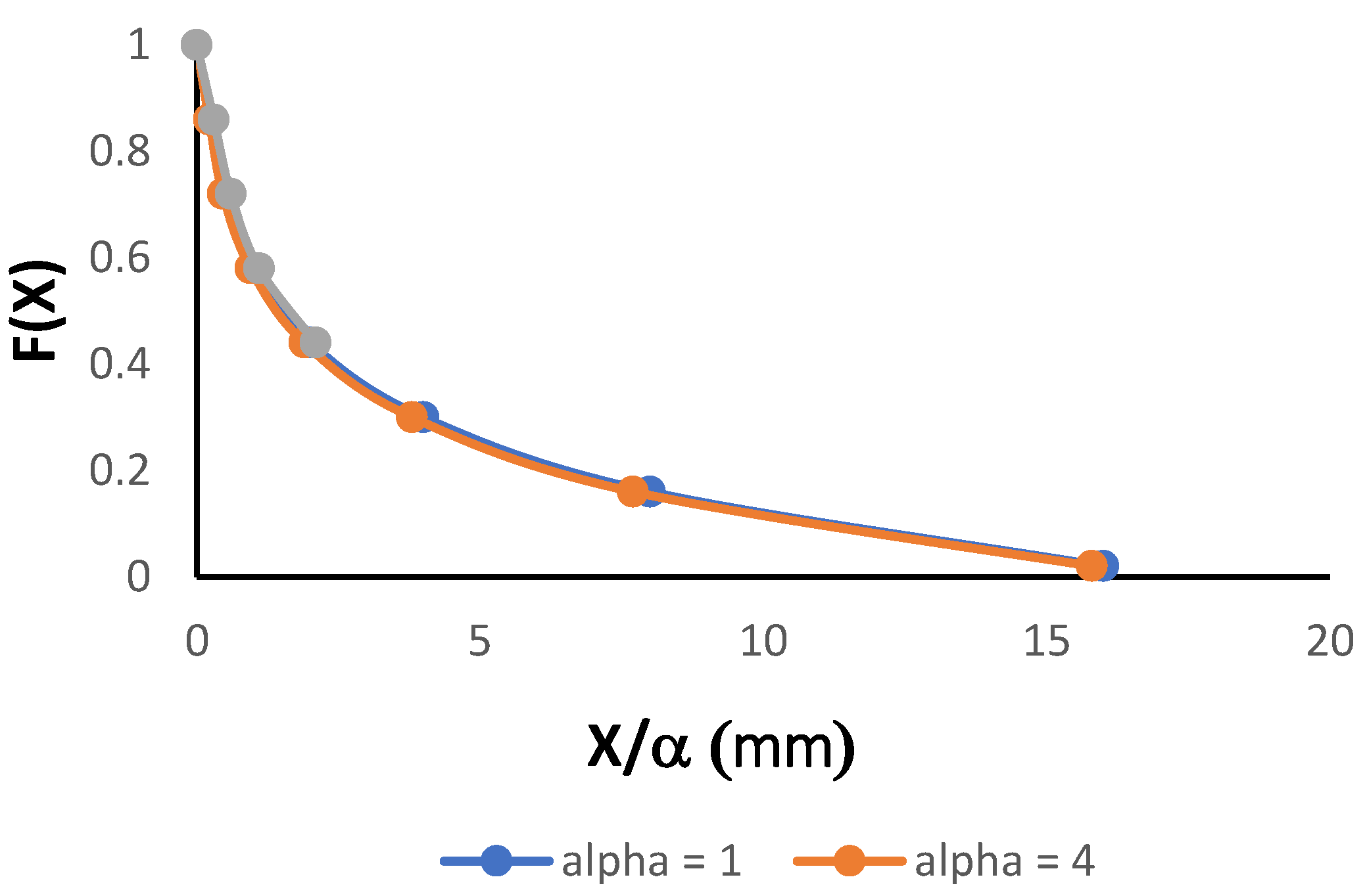
In the illustration in Figure 1, the reference distribution (always a full distribution) is defined by the blue curve. The scale factor α of the reference distribution is arbitrarily set at unity ( α = 1 ). Based on this reference distribution we can construct a second distribution, characterized by α = 4 , where each aggregate diameter X F is obtained by multiplying X o F in the reference distribution by four. This yields the orange distribution curve in Figure 1. A third distribution corresponding to α = 8 is obtained by multiplying each X o F in the reference distribution by eight, yielding the grey curve. Please note that in this case, the multiplying factor of 8 is so great that it causes many of the X(F) values of the grey curve to exceed the largest sieve aperture X m a x = 60   mm , resulting in truncation of the distribution curve at the cumulative fraction F X m a x 0.45 . The portion of the curve for X > X m a x cannot be experimentally measured Only the part of the truncated distribution corresponding to X < X m a x remains experimentally defined, but nevertheless it still conforms to scaling law (1). This shows that a set of distributions can be related by scaling law (1) regardless of whether the distributions are full or truncated.
The values of the scale factors α in a set of similar test distributions are dependent on the (arbitrary) choice of reference distribution. However, the relative values (i.e., ratios) of α corresponding to any two distributions are independent of the reference distribution. This property is sufficient to compare the relative fragmentation behavior of different soils, which is the main objective of this paper. We will later consider a class of distributions which can be scaled according to (1) without specifying any particular reference distribution.
A distinguishing characteristic of scaling relation (1) is that division of X F into the scale factor α always returns the reference value X o F . This means that for families of similar distributions, such as those in Figure 1, transformation of the variables X F to X F α causes all distributions to collapse onto the reference curve (Figure 2).
Equation (1) and Figure 1 and Figure 2 assume an ideal scaling relationship, where the scale factor α is assumed to be constant for all F . However, in practice, some distortion usually occurs. That is, when a given test distribution is compared to the designated reference distribution, the value of α relating X F and X o F at one value of F may differ from the value relating X F and X o F at another value of F . In that case, a constant average scale factor α ¯ is assumed, which, multiplied by the reference curve parameter X o F for any given F , yields an estimate of X F accurate to within some acceptable error or “residual” X F . That is
X F = α ¯ · X o F + X F  
where α ¯ is constant for all F . This relation reduces to (1) under ideal scaling, where the error X F always vanishes. Dividing the non-ideal scaling approximation (2) by α ¯ gives
X F α ¯ = X o F + X F α ¯  
which shows that the scaled distribution function X F α ¯ reduces to the reference distribution plus a distribution of residuals X F α ¯ surrounding the reference distribution.
Several methods can be used to estimate the average scale parameter α ¯ for a given distribution. We used an adaptation of the mean weight diameter (MWD), introduced by Van Bavel [27] as a frequency-weighted average aggregate diameter of a distribution. The mean weight diameter M W D F 1 ,   F 2 corresponding to the cumulative frequency interval F 1 , F 2 of a given test distribution is defined as
M W D F 1 ,   F 2 1 F 2 F 1 · F 1 F 2 X F d F
where the frequency interval F 1 , F 2 is equal to 1 ,   F X m a x in the case of truncated distributions and 1 , 0 for full distributions. To compare the frequency interval F 1 , F 2 of the test distribution to the same frequency interval of the reference distribution, a mean weight diameter M W D o F 1 , F 2 for the reference distribution is defined as
M W D o F 1 , F 2   1 F 2 F 1 · F 1 F 2 X o F d F
The mean scale factor α ¯ is then defined as the ratio of the two MWD parameters, i.e.,
α ¯ M W D F 1 ,   F 2 M W D o F 1 ,   F 2 = F 1 F 2 X F d F   F 1 F 2 X o F d F  
In the limiting case of ideal scaling governed by (1), the mean scale factor α ¯ reduces to α . This is easily seen by noting that in the ideal case, Equation (4) becomes
M W D F 1 ,   F 2 = α F 2 F 1   F 1 F 2 X o F d F = α · M W D o F 1 , F 2  
which, compared to (6), shows that α ¯ = α .
The integrals in (4) and (5) were evaluated numerically from sieving data. The integration interval ( F 1 , F 2 ) was divided into n = 1,2…N finite sub-intervals F n corresponding n = 1,2 ….N sieve size intervals, and the integrals were approximated as
F 1 F 2 X F   d F n = 1 N X F n ¯ · F n  
and
F 1 F 2 X o F   d F n = 1 N ( X o ) F n ¯ ) · F n  
Here, X F n ¯ and ( X o ) F n ¯ are the arithmetic means of the X values within the frequency interval F n for the test and reference distributions, respectively. The mean X F n ¯ for the interval was calculated as
X F n ¯ = X n + X n + 1 2  
where X n + 1 and X n are the sieve sizes bounding the frequency interval F n above and below, respectively. Likewise, the mean value ( X o ) F n ¯ of the test distribution within the frequency interval F n is calculated as
( X o ) F n ¯ = X o n + X o n + 1 2  

2.2.3. Dimensionless Representation of Similarity Relations among Distributions

In the scale model of aggregate size distributions described above (Section 2.2.2), an arbitrary distribution is chosen from among the set of experimental distributions and designated as reference distribution. Any other distribution, bounded by a particular frequency interval (F1, F2), is related to the interval (F1, F2) of the reference distribution through a scale factor α ¯ , This connection to a common reference distribution reduces comparison of different test distributions to a comparison of the respective scale factors α ¯ , even when the distributions being compared occur over different frequency intervals. However, the scaling parameter X α ¯ arising in this framework retains dimensions of length and depends on the choice of reference configuration. From the point of view of generality and mathematical elegance, a preferable scaling variable is usually one that is dimensionless and invariant under a change in reference distribution.
A scaling variable X * F with these properties arises in the special case of distributions with fixed frequency interval F 1 , F 2 , such as full distributions defined over the interval (1,0). In such cases, a dimensionless parameter X * F may be obtained from the original scaling variable X α ¯ by dividing the latter into the mean weight diameter M W D o F 1 , F 2 of the designated reference distribution, yielding
X * F X F α ¯ · M W D o F 1 , F 2  
Please note that in (12), the reference distribution parameter M W D o F 1 , F 2 is constant by virtue of the requirement of constant frequency interval F 1 , F 2 , as opposed to the earlier case of variably truncated distributions where F 1 , F 2 and therefore M W D o F 1 , F 2 vary across distributions. Since X * F   in (12) is simply the original scaling variable X α ¯ divided by a constant, graphs of F as a function X * F retain the same form as the earlier graphs of F vs. X α ¯ , such as those in Figure 2, the only difference being one of scale.
The variable X * F is not only dimensionless, but also invariant under a change in reference distribution. This is seen by combining (12) with the definition of α ¯ in (6), showing that X * F has the dual identity
X * F X F α ¯ · M W D o F 1 , F 2 = X F M W D F 1 , F 2  
Both the numerator and denominator of the variable X F M W D F 1 , F 2 on the right of (13) are determined directly from sieving experiments, and are therefore indifferent to the choice of reference distribution. The mean weight diameter M W D F 1 , F 2 in the denominator of (13) assumes the role of a “characteristic length” of the corresponding aggregate distribution, distinguishing that distribution from its neighbors. It is analogous to the characteristic structural length λ of similar porous media in the well-known Miller and Miller scaling theory of capillary phenomena [23].
The dimensionless aggregate diameter X * F X F M W D F 1 , F 2 of a given distribution does not require specifying a reference distribution, but can be related explicitly to an arbitrary reference distribution X o F if so desired. This is achieved by substituting the designated reference distribution X o F into (2), dividing both sides of (2) into M W D F 1 , F 2 and combining the result with (6). This gives
X * F = X o * F + X * F  
where X * F X F M W D F 1 , F 2 as before, X o * F X o F M W D o F 1 , F 2 is the dimensionless reference distribution, and X * F X F M W D F 1 , F 2 is the dimensionless “residual” or deviation of X * F away from X o * F .
Under ideal scaling conditions, X * F vanishes so that X * F and X o * F coincide, for all choices of reference distribution. For non-vanishing residuals, (14) shows that a dimensionless distribution X * F is equivalent to the dimensionless reference distribution X o * F plus a distribution of dimensionless residuals X * F . The magnitude of the residuals X * F depends on the degree of non-ideality of the system, and to a certain extent on the choice of reference distribution. However, (14) imposes that regardless of the choice of reference distribution, the frequency-weighted sum of residuals X * F must always vanish. This means that the distribution of residuals will always center around the designated reference distribution, rather than being displaced systematically to the left or right of it. To demonstrate this, we write the variables X * F , X o * F and X * F of (14) in terms of their full definitions, rendering (14) as
X F M W D F 1 , F 2 = X o F M W D o F 1 , F 2 + X F M W D F 1 , F 2  
Multiplying both sides of (15) by dF and integrating over the interval F 1 , F 2 gives
1 M W D F 1 , F 2 · F 1 F 2 X F d F = 1 M W D o F 1 , F 2 · F 1 F 2 X o F d F + 1 M W D F 1 , F 2 · F 1 F 2 X F d F  
Substituting the respective definitions (4) and (5) of M W D F 1 , F 2 and M W D o F 1 , F 2 into (16) gives
F 2 F 1 = F 2 F 1 + 1 M W D F 1 , F 2 · F 1 F 2 X F d F  
imposing that
1 M W D F 1 , F 2 · F 1 F 2 X F d F = F 1 F 2 X * F d F = 0  
In order for condition (18) to be satisfied, the distribution of residuals must have an equal amount of frequency-weighted positive and negative (or vanishing) residual values, requiring that a residual distribution must cross over, or coincide with, the reference distribution, as opposed to existing entirely to the right or left of it.

3. Results

3.1. Experimental Aggregate Size Distributions

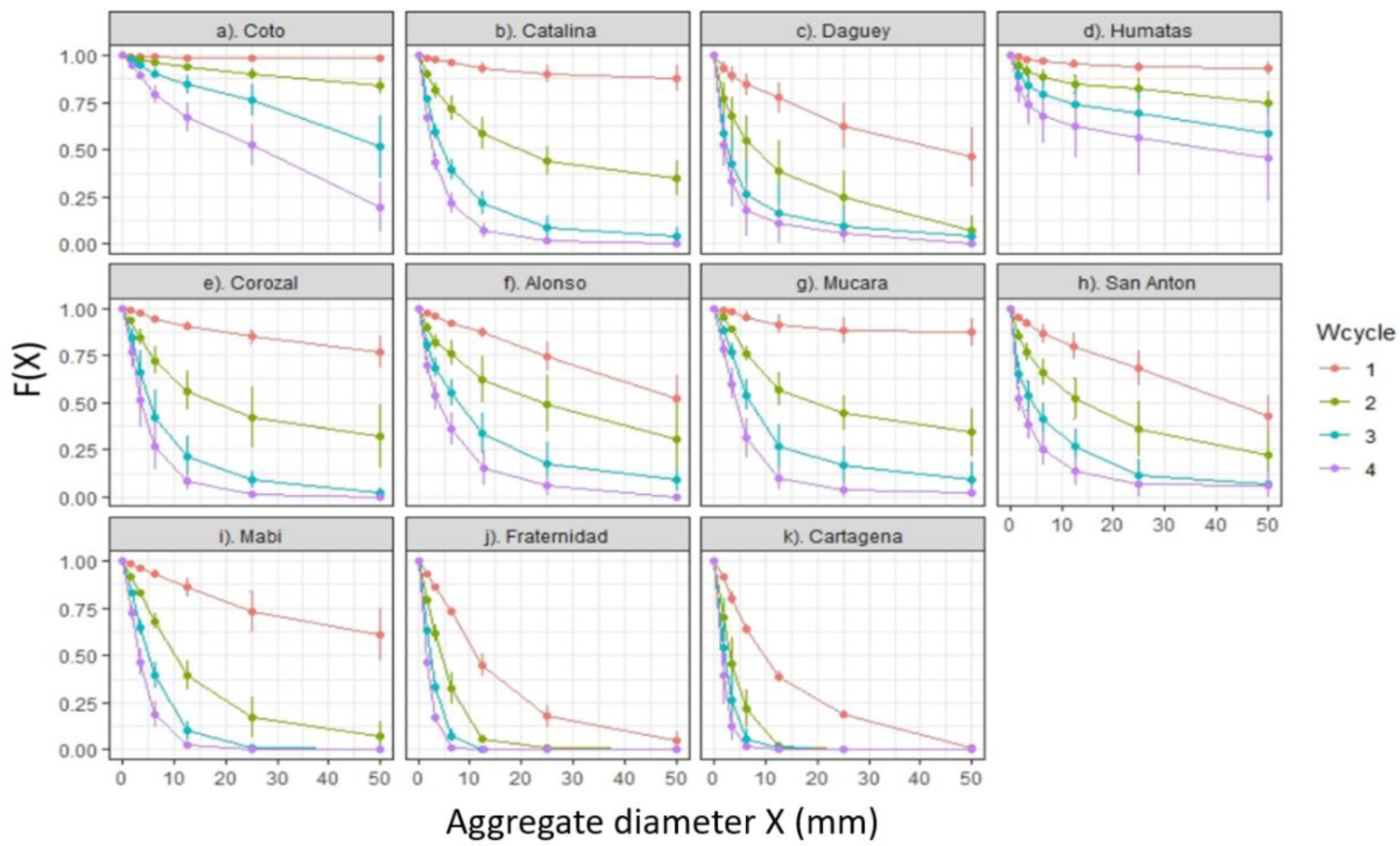
The cumulative distributions of F(X) as a function of aggregate diameter X for the 11 different soils in Puerto Rico are shown in Figure 3a–k. Each data point in the curves represents the mean of three replicate measurements. Standard deviations are represented by error bars.
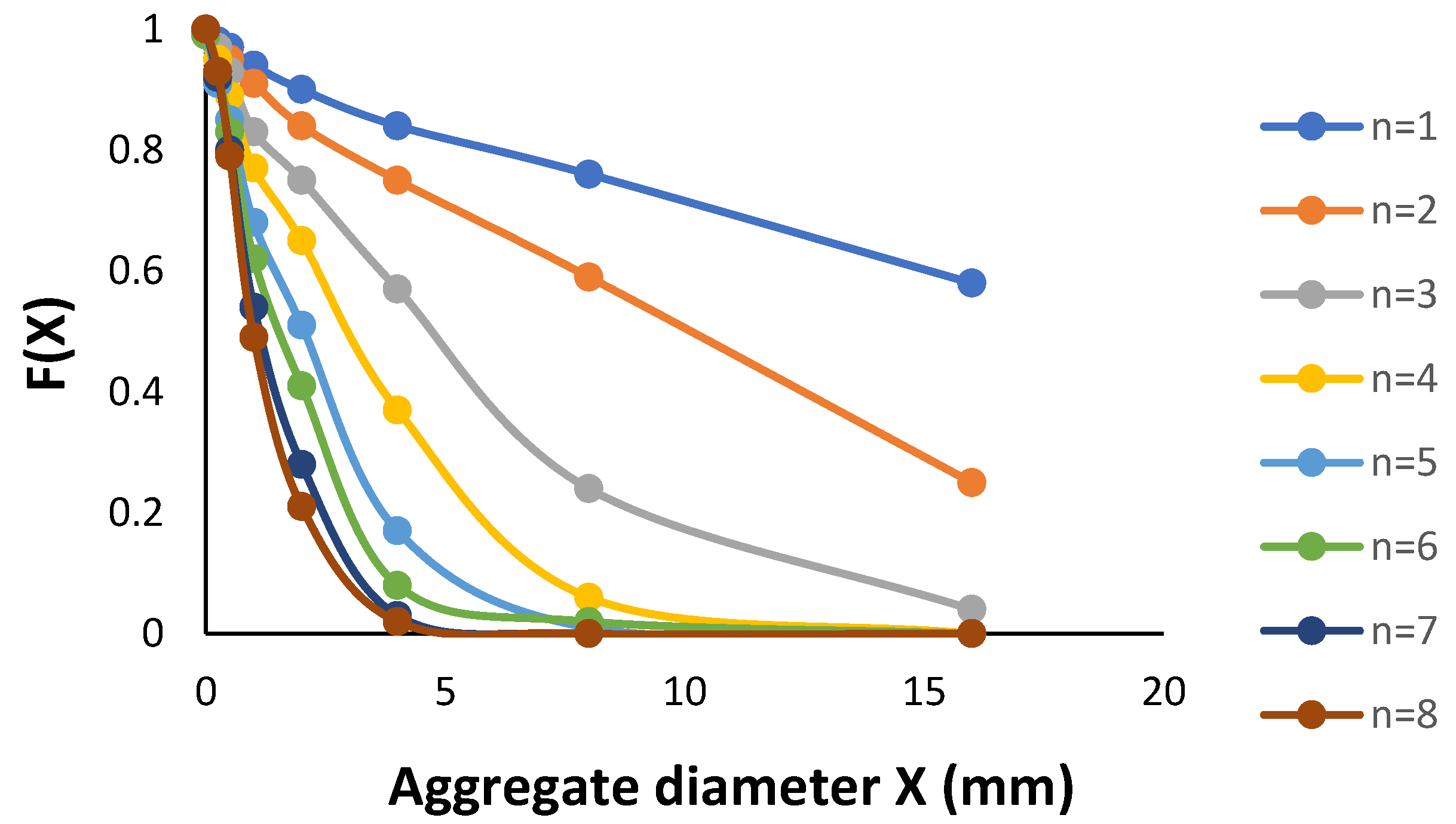
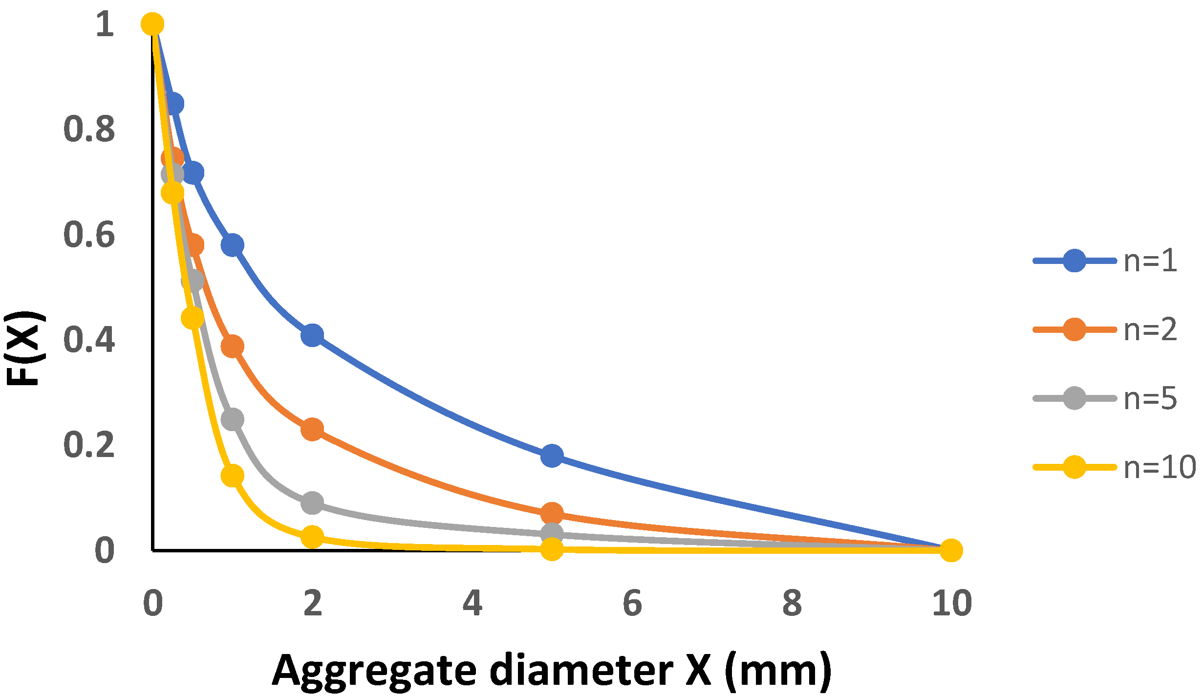
Cumulative distributions for the experiments of Shiel et al. (14) and Xu et al. (15) are shown in Figure 4 and Figure 5, respectively.
It is evident that the different aggregate size distributions in Figure 3 and Figure 4 include both full and truncated distributions, whereas in Figure 5, all distributions are full.

3.2. Representation of Aggregate Size Distributions in Terms of the Scaling Parameter X / α ¯

For all three sets of experimental data (PR, UK and PRC), we chose as a common reference distribution the experimental curve for the first wetting and drying cycle (n = 1) of the Cartagena soil in the Puerto Rico study (Figure 1). The corresponding reference scale factor value was set at α ¯ = 1. Several reasons lay behind this particular choice of reference distribution. Firstly, it was an actual experimental distribution, as opposed to a hypothetical statistical model or the result of some averaging procedure taken over all experimental data. Secondly, the Cartagena soil, a sodic Vertisol, exhibited the greatest amount of fragmentation of all Puerto Rico soils, making it a natural reference point for comparison. Thirdly, the Cartagena aggregate size distribution for n = 1 was very “well behaved”, in the sense that it was a full (as opposed to truncated) distribution, with the cumulative fraction F(X) decreasing smoothly and monotonically throughout the entire experimental sieve size range 0X ≤ 50 mm, reaching F(X) = 0 at nearly exactly the upper experimental sieve size limit X = 50 mm. The latter property avoided the difficulty of having to extrapolate the experimental curve to estimate its intercept with the X axis. The reference curve was closely approximated (R2 > 0.99) by the piece-wise analytical function
X o P = 51.74 exp 3.576   P   P < 0.915  
= 19.41   1 P   P   0.915  
Values of X o P determined analytically with the curve-fitting functions (18) and (19) were used in the numerical approximation (10) for estimating the mean aggregate diameter ( X o ) F n ¯ corresponding to a given frequency interval F n of the reference distribution.
Values of the mean scale parameter α ¯ obtained for the different soils and numbers of wetting and drying cycles (n) are listed in Table 3.
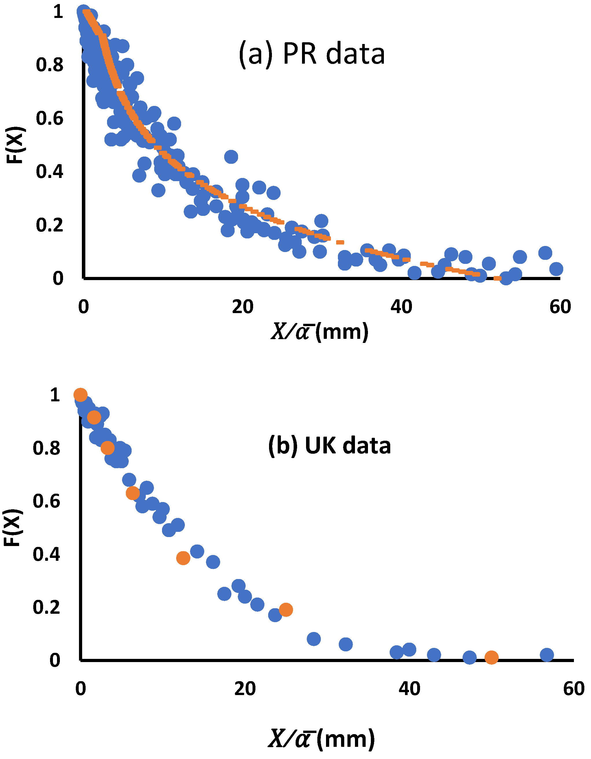
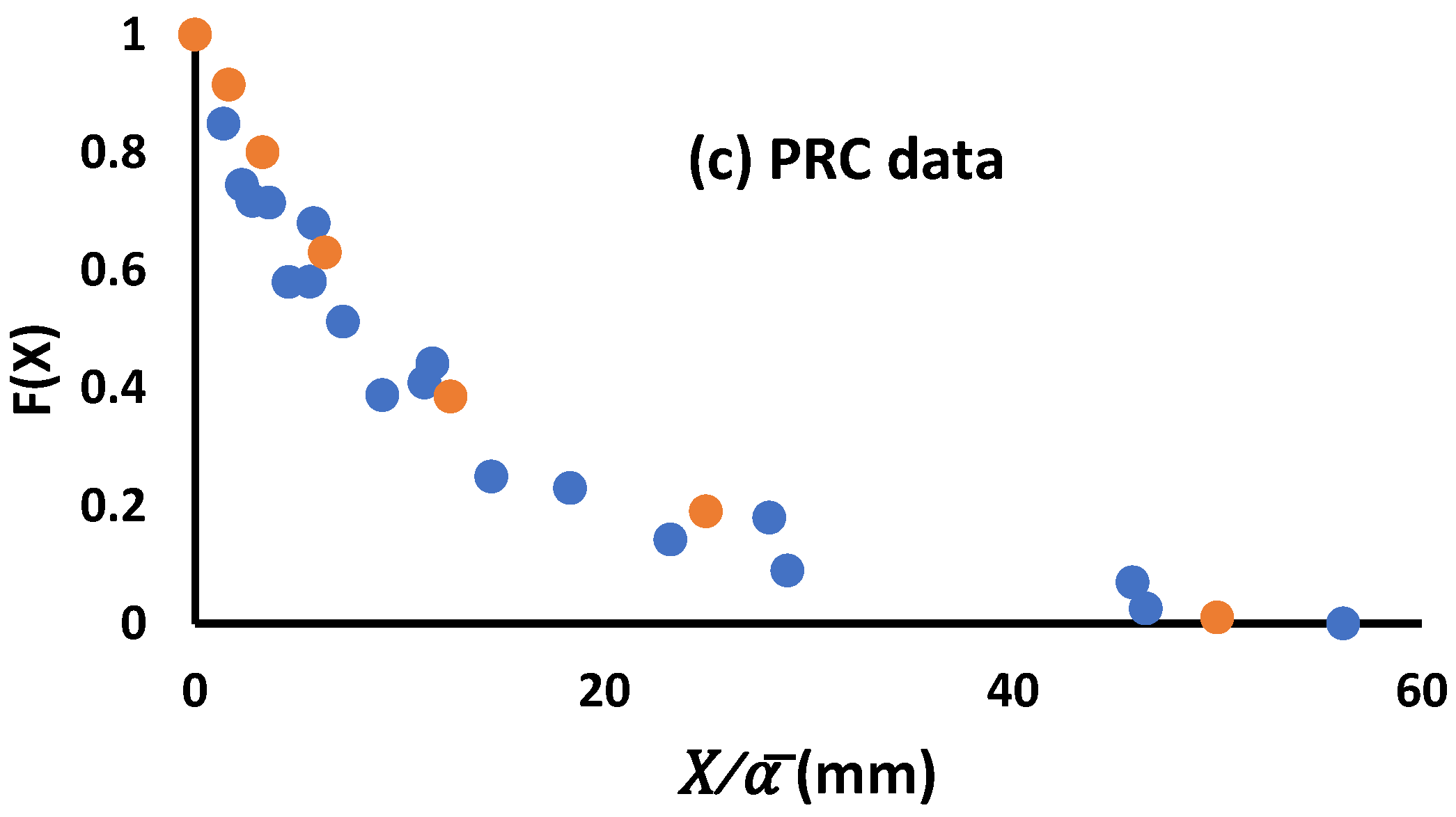
Normalized distributions constructed by plotting cumulative fractions F X against reduced aggregate diameters X α ¯ are shown for the three experimental data sets in Figure 6a–c. It can be noted that the scaled data for all three experiments collapsed reasonably well around the single Cartagena reference curve, indicated by the orange data points.

3.3. Analysis of Factors Influencing the Value of the Scale Parameter α ¯

3.3.1. Variation of α ¯ as a Function of Number of Wetting and Drying Cycles

Figure 7 gives log–log plots of the evolution of the scale factor α ¯ of the soils in all three experiments as a function of number n of wetting and drying cycles.
All of the plots were very nearly linear, indicating that the evolution of α ¯ could be approximated by the power law function
α ¯ n = α ¯ o n b  
where α ¯ o is the fitted value of α ¯ at n=1, and b is a negative exponent, equal to the slope of the log–log plots in Figure 7.
Values of α ¯ o and b for the different soils, obtained by linear regression of log α ¯ n vs. log n, are given in Table 4. The corresponding regression R2 values always exceeded 0.9.
In addition to being approximately linear, the log–log plots for the different soils in Figure 7 are nearly parallel to each other, showing that the corresponding slope b tended to remain relatively constant. With the exception of the lower blue curve in Figure 7, corresponding to the yellow-brown earth soil from PRC, the values of b listed in Table 4 ranged between −1.4 and −2.7, with a mean value of −1.96 (effectively –2) and a coefficient of variation of 0.22. This allows approximating (21) by the inverse square law
α ¯ n α ¯ o n 2  
which states that α ¯ n varies inversely with the square of the number of wetting and drying cycles.
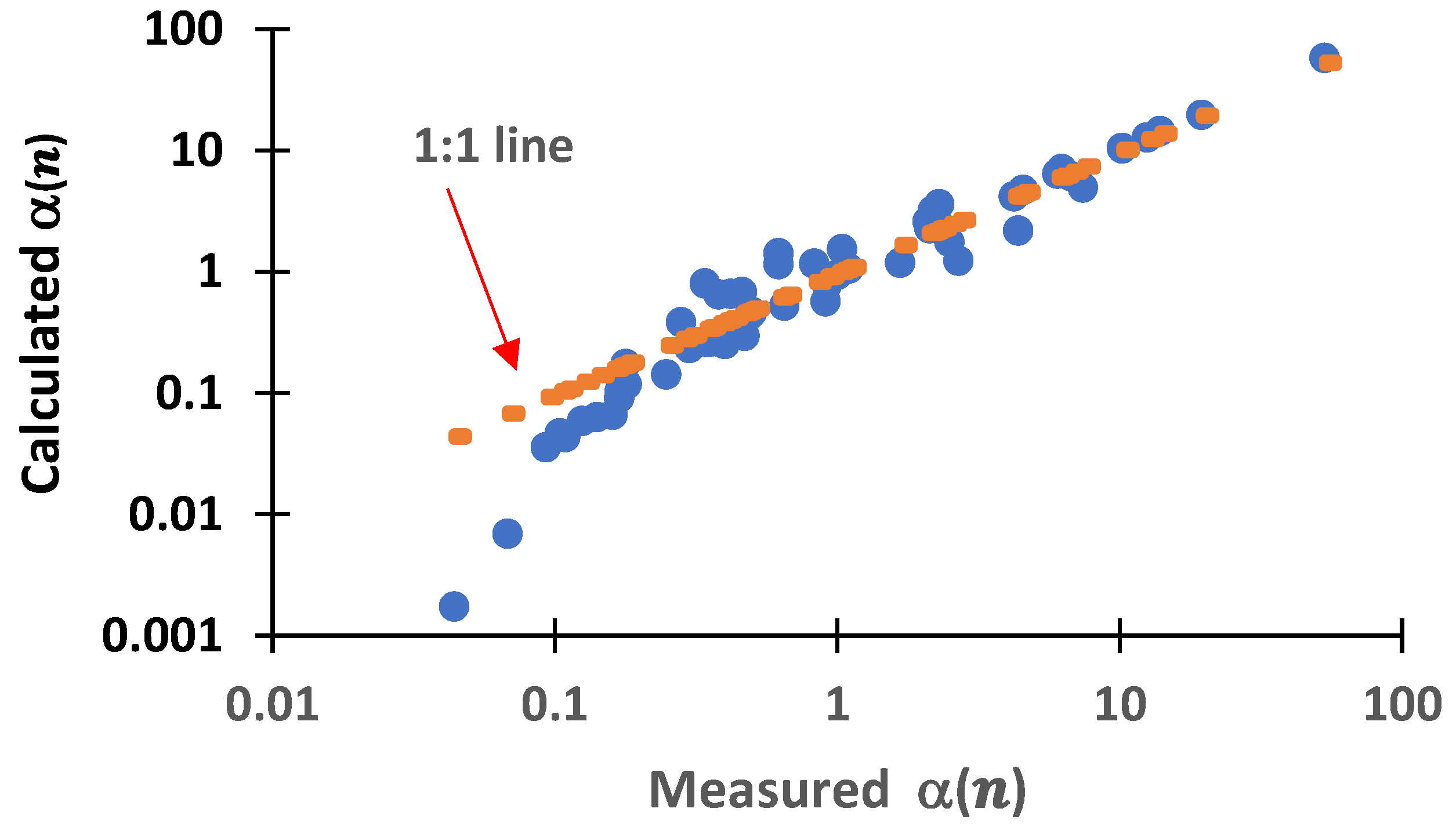
To examine this idea further, in Figure 8 we plotted values of α ¯ n estimated with Equation (22) for all soils and wetting and drying cycles against the corresponding measured values of α ¯ n listed in Table 3. The corresponding graph is given by the blue data points in Figure 8. Superimposed on this curve is the 1:1 line (orange points), which would be obtained if the predicted α ¯ n values were equal to actual values. It can be noted that the values of α ¯ n predicted by approximation (22) compared well with the 1:1 line for values of α ¯ n down to about 0.2, below which Equation (22) tended to systematically predict α ¯ n values lower than those observed. Making use of (6), the critical scale value of α ¯ = 0.2 can be converted to an absolute mean weight diameter (MWD(1,0)) by multiplying it times the mean weight diameter M W D o (1,0) of the Cartagena reference distribution (approximately 15 mm). This gives
MWD ( 1 , 0 ) = M W D o ( 1 , 0 ) × α ¯ = 15   mm × 0.2 = 3   mm
indicating that the inverse square aggregate size evolution law (22) applied reasonably well to distributions with MWD(1,0) values of 3 mm or greater, but broke down for smaller values. At these lower MWD values, much of the sieved material possibly consisted of primary particles (fine gravel and coarse sand) that no longer broke down under further wetting and drying cycles, causing erroneous predictions by (22).

3.3.2. Variation of   α ¯ as a Function of Soil Type

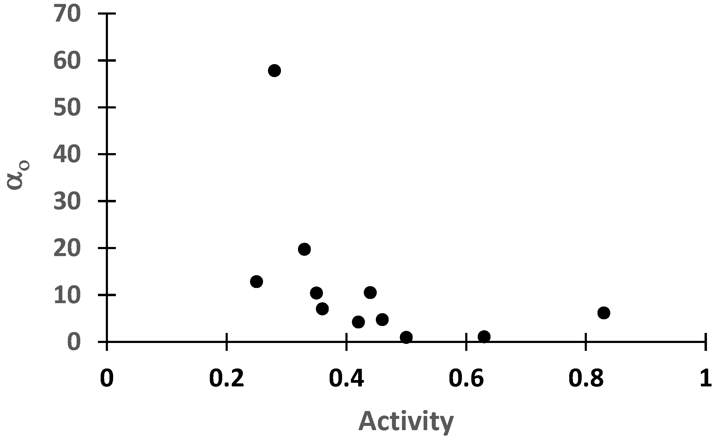
In the inverse square law (22) for a given soil, the only soil-dependent parameter is the scale factor α ¯ o , corresponding to α ¯ at n = 1. This value will in general depend on the type of soil and the initial (sampled) aggregate size distribution prior to applying the first wetting and drying cycle. If the initial aggregate size is constant, as was the case for the 11 Puerto Rico soils, then the value of α ¯ o will only depend on soil type and can be used as a measure of the relative tendency of different soils to break down under wetting and drying cycles, with smaller values of α ¯ o indicating greater fragmentation tendency. Following this line of thinking, in Figure 9, we plotted values of α ¯ o for the different PR soils against the corresponding soil activity, a parameter known to correlate positively with soil shrink–swell behavior. As expected, α ¯ o tended to decrease with increasing activity, with the tendency exhibiting a non-linear character.

3.4. Dimensionless Representation of Similar Aggregate Size Distributions

As described in Section 2.2.3 of the Materials and Methods, given a set of distributions with constant frequency range F 1 , F 2 , and given an arbitrarily designated reference distribution Xo(F), the dimensionless aggregate size distribution X * F X F M W D F 1 , F 2 is related to the dimensionless reference distribution X o * F ) X o F M W D o F 1 , F 2 as
X * F = X o * F + X * F  
where X * F X W D F 1 , F 2 is the dimensionless distribution of integrally vanishing deviations around X o * F .
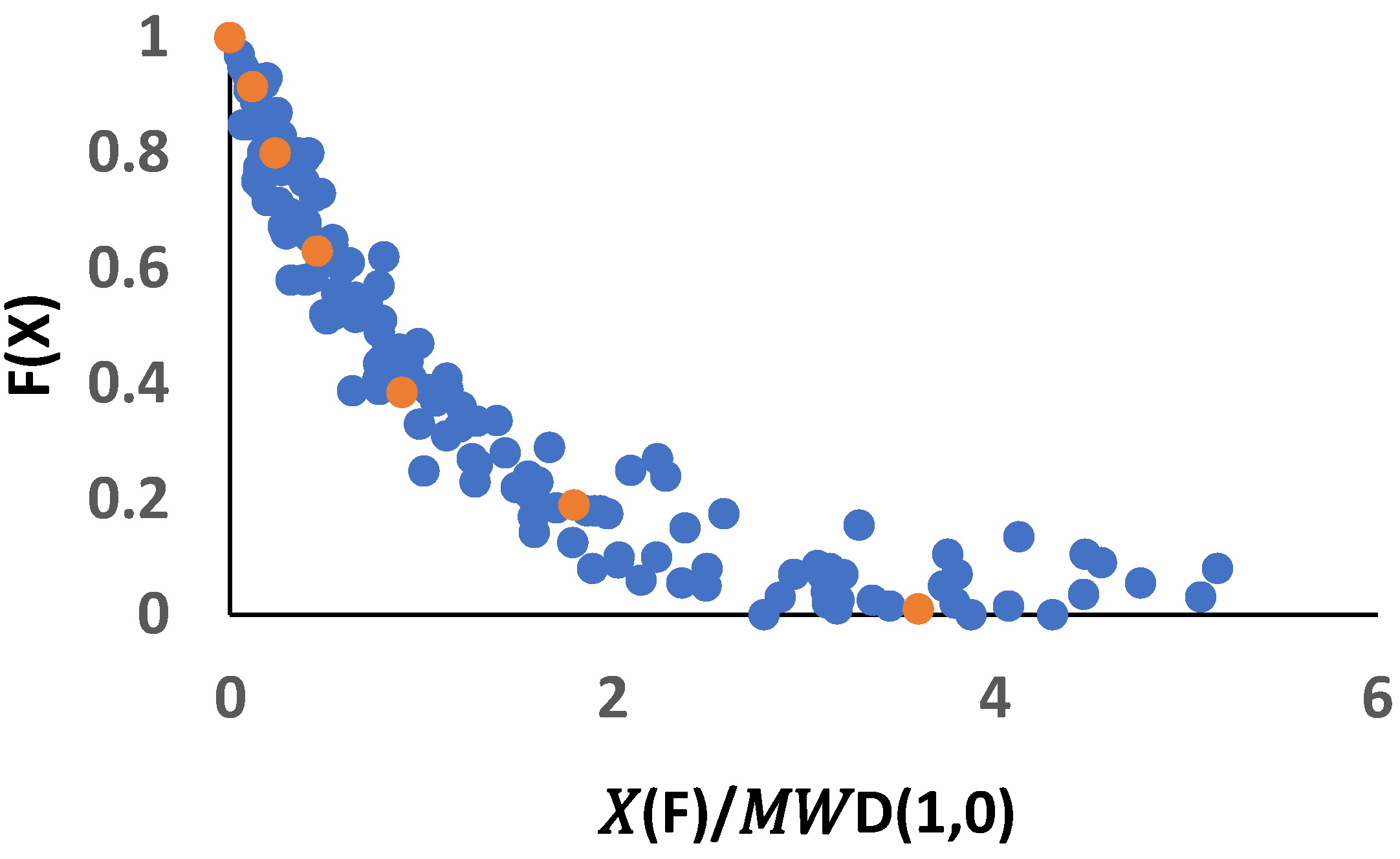
To illustrate these concepts, we pooled all the full distributions from the PR, UK and PRC data sets, with frequency intervals F 1 , F 2 = 1 ,   0 , and plotted the corresponding cumulative frequencies F as a function of X * F X F M W D 1 , 0 , as shown by the blue data points in Figure 10. Superimposed on this plot is the distribution of F vs. the dimensionless parameters X o * F X o F M W D o 1 , 0 for the Cartagena reference distribution (orange data points). It can be seen that the distribution of X * F centered quite well around the dimensionless reference distribution of X o * F , as predicted by theory.

4. Discussion

The study reported here involved only aggregate size distributions, without addressing soil hydraulic properties. Therefore, nothing can be directly concluded from our data regarding the effects of the scalable aggregate size distributions on soil hydraulic behavior. However, many studies have indicated close relations between aggregate size distributions and soil hydraulic properties [28,29,30,31,32,33,34], including scaling relationships. Wu et al. [28] measured aggregate size distributions and water retention curves in loosely packed soils with widely differing aggregate size distributions. They observed that the shapes of pore-size distributions inferred from the moisture release curves conformed well to the shapes of the aggregate size distributions. Nimmo [29] constructed a two-domain (textural and structural) model of soil water retention, assuming close correspondence between aggregate size distributions and the distribution of inter-aggregate pore sizes, allowing for variable packing densities of aggregates. The resulting moisture retention model was in good agreement with the measured water retention functions. Also noteworthy is the classic study by Sharma and Uehara [30,31], who observed Miller-type scaling relations between inter-aggregate water retention and hydraulic conductivity functions obtained in aggregate populations of different size ranges. The above literature citations are far from exhaustive, but they illustrate the value of aggregate size distributions as auxiliary data for explaining soil hydraulic properties encountered in particular situations. Nimmo [29] emphasized the need for more studies involving both types of measurements. This seems particularly true for understanding the rapid evolution of soil soil hydraulic properties immediately following tillage such as observed by Snyder et al. [1] in the plow layer of an Oxisol (Orthic Ferralsol). A significant observation in that study was the preservation of the scaling properties of sorptivity and water retention curves, which largely motivated the present investigation on scaling invariance of evolving aggregate size distributions.
As in the case of soil hydraulic properties, studies on the scaling behavior of aggregate distributions must inevitably deal with deviations from ideal scaling behavior. In applications of the Miller and Miller capillary theory to scaling of field-measured soil hydraulic properties, reference functions for water retention and/or hydraulic conductivity are typically treated as floating variables to be determined statistically by minimizing the square of residuals [24,25,26]. Tillotson and Nielsen [35] have cautioned that this runs the risk of producing mere regression parameters with questionable physical meaning. We therefore decided to base all scaling parameters on the physically measurable van Bavel mean weight diameters (MWD) of the individual distributions, in conjunction with the MWD of a reference distribution chosen from among the measured distributions of the system.

Author Contributions

Conceptualization, V.A.S.; Methodology, V.A.S. and M.A.V. Validation, V.A.S. and M.A.V.; Formal analysis, V.A.S. and M.A.V.; Investigation, V.A.S. and M.A.V.; Data curation, V.A.S. and M.A.V.; Writing—original draft preparation, V.A.S.; Writing—review and editing, V.A.S. and M.A.V.; Visualization, V.A.S.; Supervision, V.A.S.; Project administration, V.A.S.; Funding acquisition, V.A.S. All authors have read and agreed to the published version of the manuscript.

Funding

This research was partially funded by the USDA National Research Initiative (NRI) through contract 9700814, the US–Israel Binational Research and Development Fund (BARD) through contract 2794-96 and the University of Puerto Rico Agricultural Experiment Station (UPRAES).

Institutional Review Board Statement

Not applicable.

Informed Consent Statement

Not applicable.

Data Availability Statement

Not applicable.

Acknowledgments

The authors wish to acknowledge the contribution of UPRAES research assistants Vidal Santiago, Andrés López and Ramón Aponte, who spent many hours sieving and weighing aggregate samples.

Conflicts of Interest

The authors declare no conflict of interest.

References

  1. Snyder, V.A.; Rivadeneira, J.; Lugo, H.M. Temporal changes in soil structure and hydraulic properties in the plow layer of an Oxisol (Orthic Ferralsol) following tillage. Adv. Geoecol. 2000, 32, 314–324. [Google Scholar]
  2. Parvin, N.; Sandin, M.; Larsbo, M. Seedbed consolidation and surface sealing for soils of different texture and soil organic contents. Soil Tillage Res. 2021, 206, 104849. [Google Scholar] [CrossRef]
  3. Keller, J. Sprinkler intensity and soil tilth. Trans. Am. Soc. Ag. Eng. 1970, 13, 118–125. [Google Scholar] [CrossRef]
  4. Stengel, P. Cracks formation during swelling: Effects on soils structure regeneration after compaction. In Proceedings of the 11th International Conference. International Soil Tillage Organization (ISTRO), Edinburgh, UK, 11–15 July 1988; Volume 1, pp. 47–51. [Google Scholar]
  5. Or, D. Wetting-induced soil structural changes: The theory of liquid phase sintering. Water Resour. Res. 1996, 32, 3041–3049. [Google Scholar] [CrossRef]
  6. Payne, D. Some factors affecting the breakdown of soil crumbs on rapid wetting. In Proceedings of the Transactions 5th International Congress of Soil Science, Leopoldville, Democratic Republic of the Congo, 16–21 August 1954; Volume 2, pp. 53–58. [Google Scholar]
  7. Soil Physics, 4th ed.; Baver, L.D.; Garder, W.H.; Gardner, W.R. (Eds.) Wiley: New York, NY, USA, 1972. [Google Scholar]
  8. Grant, C.D.; Dexter, A.R. Air entrapment and differential swelling as factors in the mellowing of moulded soils during rapid wetting. Aust. J. Soil Res. 1990, 28, 361–369. [Google Scholar] [CrossRef]
  9. Dexter, A.R.; Kroesbergen, B. Methodolgy for determination of tensile strength of soil aggregates. J. Agric. Eng. Res. 1985, 31, 139–147. [Google Scholar] [CrossRef]
  10. Bjorneberg, D.L.; Sojka, R.E.; Aase, J.K. Pre-wetting effect on furrow irrigation erosion: A field study. Trans. Am. Soc. Agric. Eng. 2002, 45, 717–722. [Google Scholar] [CrossRef]
  11. Bityukov, K.K. Preservation of soil structure during overhead irrigation (Translation). J. Agric. Eng. Res. 1957, 2, 313–320. [Google Scholar]
  12. Gornat, B.; Goldberg, D. Effect of sprinkler irrigation intensity on the flowering and yield of peanuts grown in three different soils. Isr. J. Agric. Res. 1967, 17, 187–1911. [Google Scholar]
  13. Witte, K. Soil damages and its elimination and its elimination by sprinkling irrigation. La Irrig. A Pioggia Italy 1956, 3, 106–126. [Google Scholar]
  14. Shiel, R.S.; Adey, M.A.; Lodder, M. The effect of successive wet/dry cycles on aggregate size distribution in a clay texture soil. J. Soil Sci. 1988, 39, 71–80. [Google Scholar] [CrossRef]
  15. Xu, J.; Tang, Y.; Shou, J. Effect of drying-wetting cycles on aggregate breakdown for yellow-brown earths in karst areas. Geoenviron. Disasters 2017, 4, 20. [Google Scholar] [CrossRef]
  16. Griffith, A.A. The phenomena of rupture and flow in solids. Proc. Phil. Tans. R. Soc. Lond. Sect. A 1921, 221, 163–198. [Google Scholar]
  17. Memhard, D.; Brocks, W.; Fricke, S. Characterization of ductile tearing resistance by an energy dissipation rate. Fatigue Fract. Eng. Mater. Struct. 1993, 16, 1109–1124. [Google Scholar] [CrossRef]
  18. Day, P.R. Particle fractionation and particle size analysis. In Methods of Soil Analysis. Agronomy Monograph No. 9. Part 1; Black, C.A., Ed.; Physical and Mineralogical Methods; American Society of Agronomy: Madison, WI, USA, 1965. [Google Scholar]
  19. Kettler, T.A.; Doran, J.W.; Gilbert, T.L. Simplified method for soil particle-size determination to accompany soil-quality analyses. Soil Sci. Soc. Am. J. 2001, 65, 849–852. [Google Scholar] [CrossRef]
  20. ASTM. Standard Test Methods for Liquid Limit, Plastic Limit, and Plasticity Index of Soils; ASTM D4318-17e1; ASTM International: West Conshohocken, PA, USA, 2017. [Google Scholar]
  21. B.S. 1377-2; Methods of test for soil for civil engineering purposes. Classification Tests. Civil engineering, Earthworks; Excavations; Foundation construction; Underground works. British Standards Institution: London, UK, 1990.
  22. FAO. Standard Operating Procedure for Soil Organic Carbon. In Walkley-Black Method: Titration and Colorimetric Method; Glosolan SOP 2; Global Soil Laboratory Network: FAO, Rome, 2020. [Google Scholar]
  23. Miller, E.E.; Miller, R.D. Physical theory for capillary flow phenomena. J. Appl. Phys. 1956, 27, 324–332. [Google Scholar] [CrossRef]
  24. Warrick, A.W.; Mullen, G.J.; Nielsen, D.R. Scaling field-measured soil hydraulic properties using a similar media concept. Water Resour. Res. 1977, 13, 355–362. [Google Scholar] [CrossRef]
  25. Simmons, C.S.; Nielsen, D.R.; Biggar, J.W. Scaling of field measured soil water properties. Hilgardia 1979, 47, 77–174. [Google Scholar] [CrossRef]
  26. Russo, D.; Bresler, E. Scaling soil hydraulic properties of a heterogeneous field. Soil Sci. Soc. Am. J. 1980, 44, 681–683. [Google Scholar] [CrossRef]
  27. Van Bavel, C.H.M. Mean weight-diameter of soil aggregates as a statistical index of aggregation. Soil Sci. Soc. Am. Proc. 1950, 14, 20–23. [Google Scholar] [CrossRef]
  28. Wu, I.; Vomocil, J.A.; Childs, S.W. Pore size, particle size, aggregate size, and water retention. Soil Sci. Soc. Am. J. 1990, 54, 952–956. [Google Scholar] [CrossRef]
  29. Nimmo, J.R. Modeling structural influences on soil water retention. Soil Sci. Soc. Am. J. 1997, 61, 712–719. [Google Scholar] [CrossRef]
  30. Sharma, M.L.; Uehara, G. Influence of Soil Structure on Water Relations in Low Humic Latosols: I. Water retention. Soil Sci. Soc. Am. J. 1968, 32, 765–770. [Google Scholar] [CrossRef]
  31. Sharma, M.L.; Uehara, G. Influence of Soil Structure on Water Relations in Low Humic Latosols: II. Water movement. Soil Sci. Soc. Am. J. 1968, 32, 770–774. [Google Scholar] [CrossRef]
  32. Guber, A.; Rawls, W.J.; Shein, E.V.; Pachepsky, Y. Effect of soil aggregate size distributions on water retention. Soil Sci. 2003, 168, 223–233. [Google Scholar] [CrossRef]
  33. Slawinski, C.; Witkowska-Waltczak, B.; Lipiec, J.; Nosalewicz, A. Effect of aggregate size on water movement in soils. Int. Agrophysics 2011, 25, 53–58. [Google Scholar]
  34. Lipiec, J.; Walcza, R.; Witkowska-Walczak, R.; Nosalewicz, A.; Slowiáska-Jurkiewicz, A.; Slawinski, C. The effect of aggregate size on water retention and pore structure of silt loam soils of different genesis. Soil Tillage Res. 2007, 97, 239–246. [Google Scholar] [CrossRef]
  35. Tillotson, P.R.; Nielsen, D.R. Scale factors in soil science. Soil Sci. Soc. Am. J. 1984, 48, 953–959. [Google Scholar] [CrossRef]
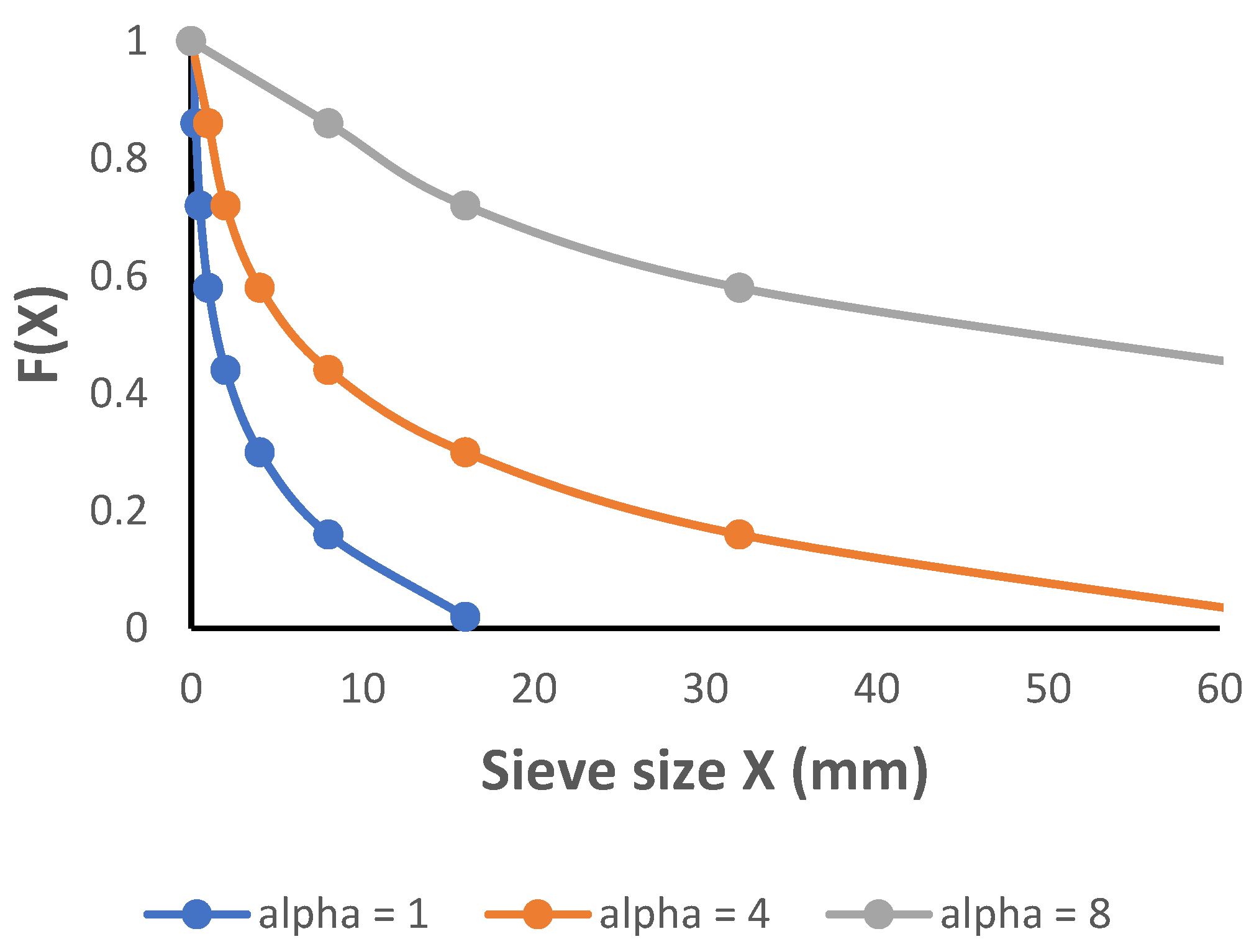
Figure 1. Hypothetical family of similar aggregate distributions conforming to scaling law (1), with scale factor values of α = 1 , 4   and   8 , respectively.
Hydrology 09 00030 g001
Figure 2. Reduction of the family of distributions in Figure 1 to a single distribution of F as a function of the scaled aggregate diameter X/α.
Hydrology 09 00030 g002
Figure 3. (ak) Aggregate size distributions of different soils from Puerto Rico as a function of number of wetting and drying cycles. The error bars represent standard deviations of three replicate samples.
Hydrology 09 00030 g003
Figure 4. Aggregate size distributions for a pello-alluvial gley soil from the UK as a function of the number (n) of wetting and drying cycles. Graphs are reconstructed from tabular data provided in Shiel et al. [14]. Each data point is the mean of four replications.
Hydrology 09 00030 g004
Figure 5. Aggregate size distributions for a yellow brown earth soil from China as a function of the number (n) of wetting and drying cycles. Graphs are reconstructed from tabular data provided in Xu et al. [15]. Each data point is the mean of five replications.
Hydrology 09 00030 g005
Figure 6. Scaled aggregate size distributions for all soils and numbers of wetting and drying cycles, obtained by plotting F(X) as a function of X / α . The reference distribution, corresponding to the Cartagena soil from Puerto Rico after one wetting and drying cycle, is indicated in each graph by the orange data points.
Hydrology 09 00030 g006aHydrology 09 00030 g006b
Figure 7. Log–log plots of scale factor α ¯ n as a function of number (n) of wetting and drying cycles, for all soils in the study.
Hydrology 09 00030 g007
Figure 8. Scale factor α ¯ n calculated with inverse square law Equation (22) plotted as a function of measured values of α ¯ n listed in Table 4. The 1:1 line is indicated by orange data points.
Hydrology 09 00030 g008
Figure 9. Scale parameter α ¯ o for PR soils plotted as a function of soil activity.
Hydrology 09 00030 g009
Figure 10. Plot of F(X) vs. the reduced variable X/MWD(1,0) for pooled full distributions from all experiments (blue dots). The orange dots correspond to the Cartagena reference distribution.
Hydrology 09 00030 g010
Table 1. Classification of soils in Puerto Rico study according to USDA Soil Taxonomy.
Soil SeriesClassification According to USDA Soil Taxonomy
CotoVery-fine, kaolinitic, isohyperthermic Typic Eutrustox
CatalinaVery-fine, ferruginous, isohyperthermic Typic Hapludox
DagueyVery-fine, kaolinitic, isohyperthermic Inceptic Hapludox
HumatasVery-fine, parasesquic, isohyperthermic Typic Haplohumults
CorozalVery-fine, parasesquic, isohyperthermic Typic Hapludults
AlonsoVery-fine, parasesquic, isohyperthermic Oxic Dystrudepts
MúcaraCoarse-loamy, vermiculitic, isohyperthermic Dystric Eutrudepts
San AntónFine-loamy, mixed, superactive, isohyperthermic Cumulic Haplustolls
MabíVery-fine, mixed, active, isohyperthermic Aquic Hapluderts
FraternidadFine, smectitic, isohyperthermic Typic Haplusterts
CartagenaFine, mixed, superactive, isohyperthermic Sodic Haplusterts
Table 2. Basic properties of soils in the Puerto Rico study.
SoilSeriesSoil Particle Size Classes (Percent by Mass)Bulk Density(Mg m−3)Atterberg LimitsCoefficient of ActivityOrganic Matter Content (Percent)
SandSiltClayLiquid LimitPIasticity Index
Coto294671.4649190.283.86
Catalina620741.2166190.251.24
Daguey2322551.4362230.421.42
Humatas1536501.2349170.332.87
Corozal2018611.3958220.352.15
Alonso2322551.3058200.362.16
Múcara3418481.5155210.442.67
San Antón3926341.6240160.472.41
Mabí402139--64320.822.15
Fraternidad3119501.5162320.642.47
Cartagena2413631.4564310.492.42
Table 3. Scale parameter α ¯ for different soils and numbers (n) of wetting and drying cycles.
Soiln = 1n = 2n = 3n = 4n = 5n = 6n = 7n = 8n = 10
Coto53.213.96.022.3
Catalina12.52.180.6170.34
Daguey4.221.080.50.35
Humatas19.57.424.382.69
Corozal10.22.090.620.38
Alonso6.242.500.920.49
Múcara10.22.260.830.42
San Antón4.551.670.650.47
Mabí6.741.040.460.28
Fraternidad1.10.380.180.16
Cartagena10.2980.1730.125
Gley soil (UK)2.120.9140.40.2480.1690.1410.1040.093
Y.-Br. earth (PRC)0.1780.109 0.068 0.044
Table 4. Fitted parameters α ¯ o and b of Equation (21) listed for different soils.
Soil α ¯ o B
Oto57.8−2.2
Catalina12.8−2.69
Daguey4.19−2.03
Humatas19.7−1.41
Corozal10.4−2.45
Alonso7.03−1.84
Múcara10.5−2.30
San Antón4.73−1.69
Mabí6.13−2.33
Fraternidad1.06−1.46
Cartagena0.94−1.52
Gley soil (UK)2.28−1.57
Y.-Brown earth (PRC)0.173−0.59
Publisher’s Note: MDPI stays neutral with regard to jurisdictional claims in published maps and institutional affiliations.