Abstract
This paper presents a system for supporting hydropower production on mountainous areas. The system couples the outputs of a numerical weather prediction model and a snow melting and accumulation temperature-based model. Several procedures are presented for interpolating meteorological variables and calibrating and validating model parameters that can be generalized to any other mountainous area where the estimation of current and forecasted snow water equivalent and melting amount is required. The system reliability has been assessed through the validation of three components: spatial interpolation of meteorological data, mathematical modeling, and quantitative meteorological forecast. The results show that good accuracy of meteorological data spatial interpolation can be achieved when the data from snow gauges are used for assessing the precipitation lapse rate at higher altitudes, and the temperature lapse rate is computed from data at each time step. The temperature-based hydrological model proved to be effective in simulating lake inflow water volume and energy production. No clear result has been found for snow melt forecast due to the difficulties in providing reliable quantitative weather forecast in complex alpine area.
1. Introduction
Since late XIX century, hydropower production is constantly increasing all around the world [1], with production being around 15% of all global electricity [2]. The combination of different upstream river catchments characteristics, mainly in terms of hydrology, climatology, and topography, influences the potential of hydropower production [3,4,5]. Climate change may also modify this hydropower potential by greatly impacting the snow dynamics with shifts in the time of the melt water volumes, as well as the patterns and amount of rainfall [6,7].
Thus, an enhanced knowledge of the snow dynamics and their spatial variability is fundamental for monitoring and forecasting hydropower production, as well as for river flow hydrograph monitoring and the management of water resources in Alpine catchments.
In the literature, a large amount of research has been conducted on snow dynamics modeling and monitoring with ground and satellite data [8,9,10,11]. However, especially snowmelt modeling is still challenging, mainly due to the scarcity and accuracy of meteorological information at high elevations, particularly for precipitation underestimation [12,13] and to the difficulties in monitoring and understanding the snow processes over complex surfaces and densely forested area [14,15]. Hence, snowmelt simulation is usually based on temperature degree factors and energy balance models [16,17,18].
The air temperature-based models are the most used for operational purposes (e.g., hydropower production forecast) [19], mainly due to the wide availability of air temperature data in respect to wind and radiation information and an easier computational capability without losing accuracy. These models are based on a relationship between air temperature and a snowmelt degree-day factor [18] when a temperature threshold for snow melt is reached. This degree-day factor is a highly variable coefficient which might be influenced by catchments topography [20], with higher values with increasing altitude, snow density and sun exposure [21,22], while lower values are expected in highly forested areas [23]. Moreover, a seasonal trend of the factor can also be present with a decrease in its values due to the increase in the surface albedo [24]. The degree day factor has been calibrated locally against ground-observed snow water equivalent (SWE) data or by merging ground SWE with ground snow depth data [19,23]. Satellite data of snow coverage areas can be used for model calibration to ensure a higher spatial consistency of model estimates and accuracy in non-gauged areas, improving not only the snow coverage distribution but also the SWE and the runoff, especially during the melt season [8,20,25,26,27,28]. However, as snow cover satellite data provides only the geographical distribution of snow presence or absence, the SWE estimation relies only on models estimates. Another disadvantage of satellite data, either at high (Sentinel 20 m or Landsat at 30 m) or low spatial resolutions (MODIS at 500 m) [29], is related to the missing information with cloud cover [30,31] or over densely forested areas [8].
Moreover, in the operational applications, especially for hydropower production, the monitoring of SWE or runoff should be joined by the forecasts of the same variables, coupling hydrological and weather forecast models [32,33]. Weather forecasts in Alpine and generally mountainous regions are challenging due to the effects of complex orography on atmosphere thermodynamics from mesoscale to microscale [34]. In Southern Tyrol, an area in the Eastern Italian Alps, there is the presence of several ridges and valleys, positioned on east–west or north–south axes, leading to specific micro-climates, depending on the interaction with large scale weather systems, different irradiance patterns and other local effects. For this reason, an accurate forecast requires high resolution local area models (LAM), built with specific microphysics schemes. A dense observational network is also needed to accurately describe the different microclimates [35]. These uncertainties are then reflected into the hydrological simulation, with the propagation of meteorological forecast errors into the SWE and runoff forecasts [32,33,36]. An improvement in the processes’ estimates may come from the use of probabilistic forecasts, widely used in hydrological applications in the last years [37,38], while very few applications are available for the SWE forecast in high elevation catchments [33]. Their main advantage is linked to the possibility of representing the meteorological forecast uncertainty into the hydrological application.
In this study, we aim at monitoring and forecasting the hydropower production for eight small river basins underlying a hydroelectric power plant in the Italian Alps in the Province of Bolzano. The distributed hydrological FEST-EWB (Flash-flood Event-based Spatially distributed rainfall–runoff Transformation Energy Water Balance model) [8,39] model estimates of SWE have been calibrated against ground measurements of snow height and validated with satellite MODIS data of area coverage. The estimates of model hydropower productions have then been compared at monthly scale with measured data at each powerplant. The calibrated model has been finally coupled with ensemble meteorological forecasts based on the WRF-ARW (Weather Research and Forecasting Advanced Research WRF) model [40] to provide SWE and energy production for a week in advance. The quality of these forecasts is verified for the different basins.
The main innovation points are:
- Improvement of the interpolation technique of ground precipitation measurements considering the altitude;
- Forecast of the energy production at weekly scale using a distributed snow model coupled with ensemble weather forecast;
- The local application to the Bolzano province.
2. Materials and Methods
2.1. Case Study Area and Data
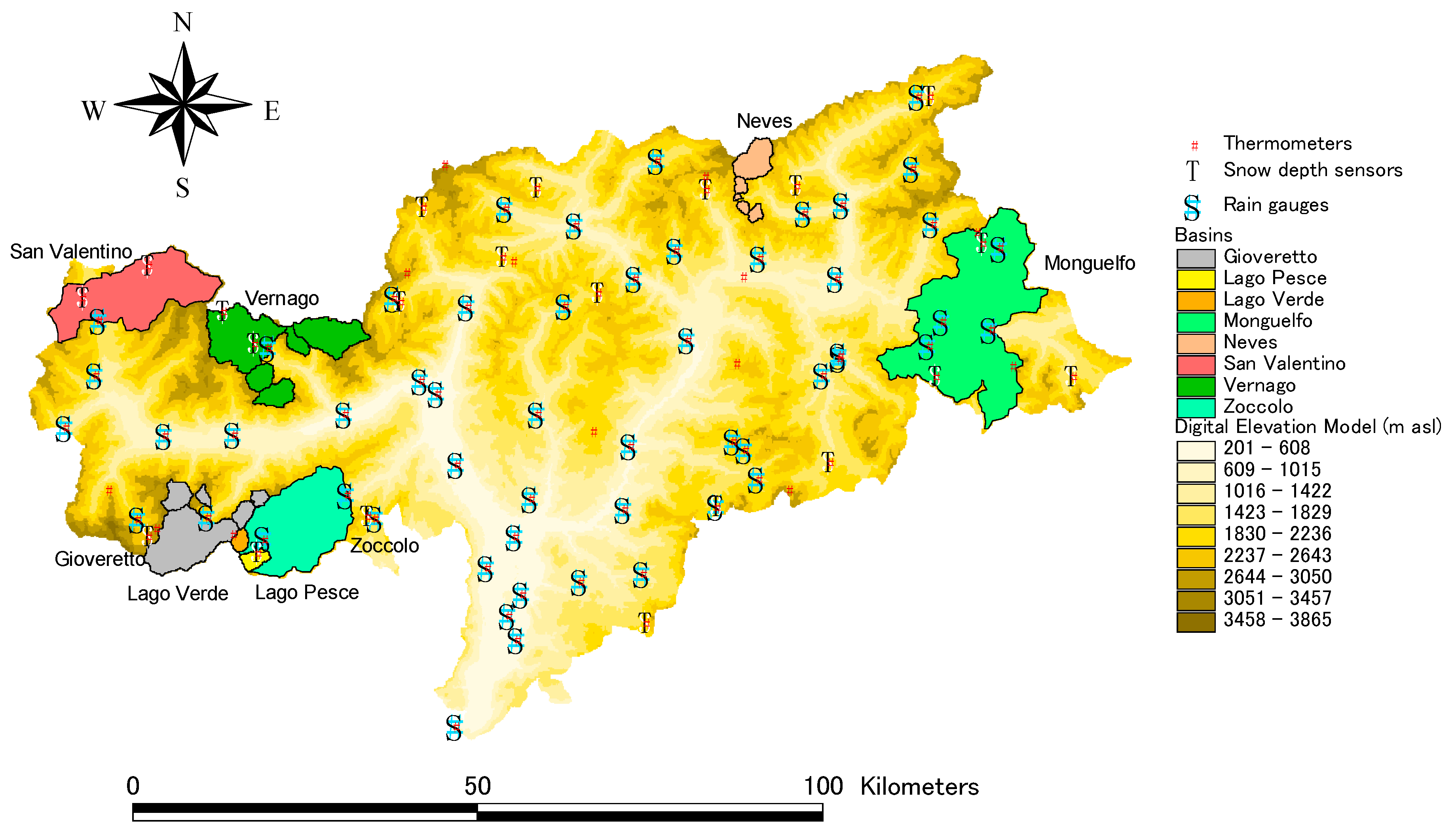
The case study area is the Province of Bolzano (Northern Italy), which covers an area of about 7400 km2 (Figure 1). The basin is an Alpine catchment, characterized by almost entirely mountainous areas with high elevation gradients. Three main rivers shape the area: (i) in the western part, the Adige river; (ii) in the northern part, the Isarco; and (iii) in the eastern part, the Rienza river. The runoff regime is snow and glacier dominated. The climate is characterized by dry winters and high snowmelt during the spring season [41,42].
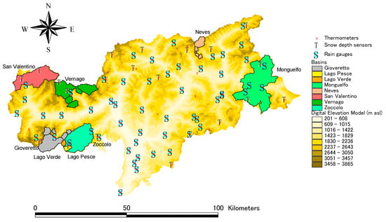
Figure 1.
Case study area with the pluviometric, thermometer and nivometric stations, the hydropower plants and the relative basins.
Eight smaller river basins are identified as underlying a hydroelectric power plant. In the Southern part of the area are located the Lago Verde and Lago Pesce basins, the smallest ones and at the highest elevations. These are in turn sub-basins of the Zoccolo basin. Nearby, the Gioveretto catchment is also located, which is characterized by not only its natural river catchment area, but it also includes a series of connected basins which directly supply water to the power plant. A similar hydraulic scheme is also observable in the northern basins of Neves and Vernago. In the northwest, the San Valentino basin is located, while in the eastern area is the Monguelfo one, which is the largest and the lowest basin. Table 1 reports a list of relevant information about these catchments.

Table 1.
The Alperia hydropower plants and the relative basins along with their energy production.
2.1.1. Energy Production at Hydropower Power Plants and Lake Reconstructed Inflow
Alperia Greenpower Srl (www.alperiagroup.eu, accessed on 27 December 2021) manages 34 hydroelectric power stations in the South Tyrol mountains, producing an average of 4500 GWh of energy every year. For this analysis, eight power stations (Table 1) are considered, which receive water from the natural and connected basins (Figure 1). In the considered hydrographic catchment, irrigation is not present and drinking water uses are negligible, so the management of the reservoirs can be simulated as completely oriented to hydropower production.
Monthly energy production is available at the three powerplants of Naturno, Glorenza and Lasa from 2006 to 2020; while reconstructed inflow to the power plants lakes is available for all the eight basins from 2017 to 2021.
2.1.2. Ground Meteorological and Nivometric Data
Meteorological stations are available from the Bolzano Province network (Figure 1): 87 of them provide air temperature, and 48 also provide precipitation. All the data are available at an hourly resolution from 2016 to 2021 from the website http://meteobrowser.eurac.edu/ (accessed on 10 October 2020). Higher total yearly precipitation values are observed in the Neves, Gioveretto and Lago Verde and Pesce basins (1200 mm), while the lowest ones are in the western part (San Valentico catchment) around 1000 mm (Table 1).
Moreover, snow depth data are also available from 21 stations from 2016 to 2019 (Figure 1).
2.1.3. Satellite Data of Snow Coverage
For the analyzed period from 2016 to 2019, a total of 101 images at 500 m spatial resolution are obtained from satellite data by the MODIS Terra MOD10_A1 daily product images (MODIS Snow Cover Daily L3 Global 500m Grid) from the MODIS/NSIDC website archive http://nsidc.org/index.html (accessed on 20 May 2020).
The MODIS instrument is onboard two satellites, namely, Terra and Aqua, while in this study, only the Terra MODIS data are used because the Aqua MODIS band at 1.6 micron, which enhances the difference between snow and clouds, was broken just after satellite launch. The MODIS snow retrieval algorithm [43] is based on the difference between the infrared reflectance of snow in visible and short-wave wavelengths, where snow has a strong reflectance in the visible bands and strong absorption in the short-wave bands, allowing for the distinction with clouds. Snow MODIS data are provided as now cover area percentage, which is particularly useful for sensitivity during the melting season [44].
2.2. Methodology
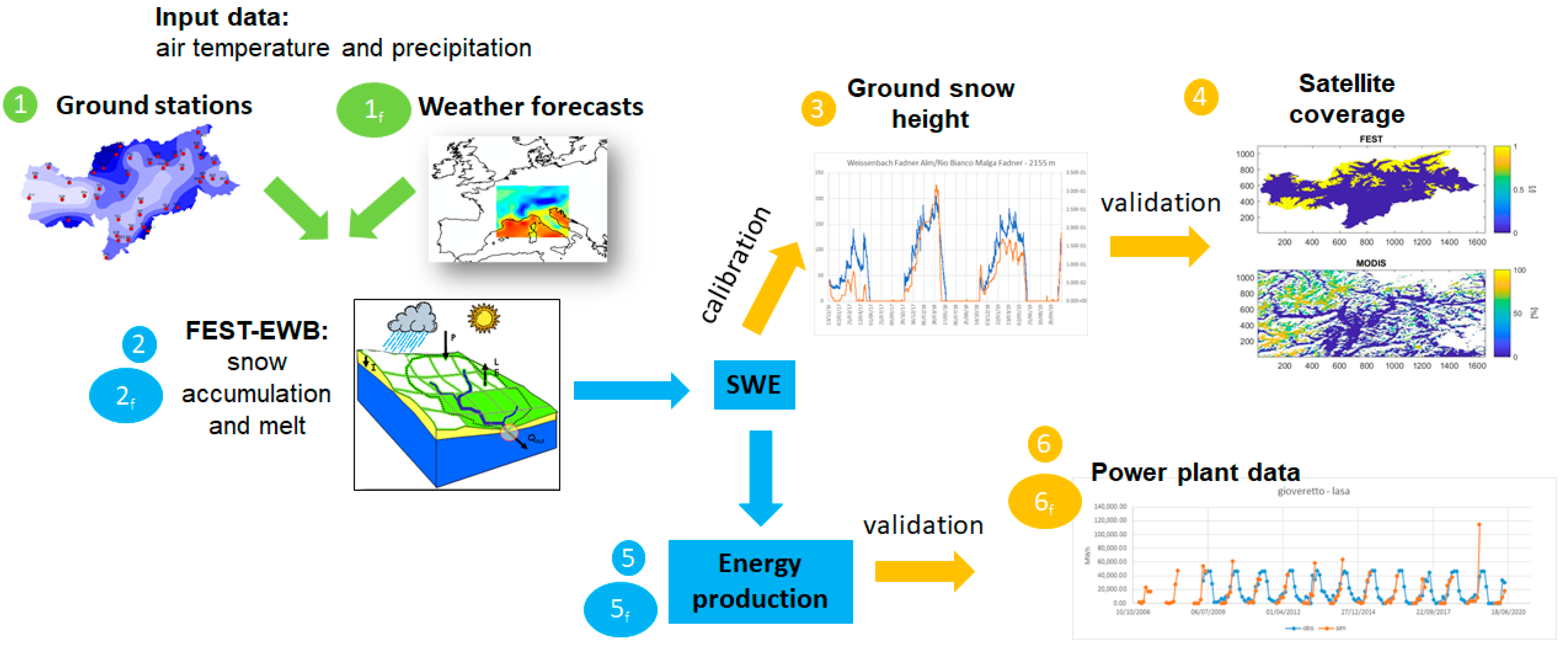
The scheme of the implemented methodology is reported in Figure 2. The FEST-EWB snow model is firstly run with ground meteorological stations data of rainfall and air temperature (step 1) to calibrate the snow accumulation and melt parameters (step 2) in comparison to the modelled SWE with local ground measured snow height (step 3). The snow model parameters are then validated against MODIS satellite data of snow cover area (step 4) over the whole Bolzano province. The modeled SWE is then transformed into potential hydropower production (step 5) and compared with the measured data at the different power plants (step 6). Finally, the WRF meteorological forecasts (step 1f) are used as inputs to the FEST-EWB model (step 2f) to generate hydro-meteorological forecasts of SWE and energy production (step 5f). Uncertainties of the forecasted variables is assessed against observed data (step 6f).
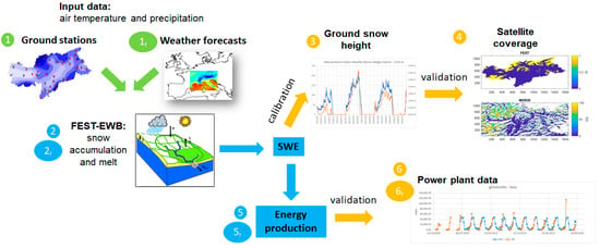
Figure 2.
Methodological scheme: The numbers refer to the calibration and validation procedures with the observed meteorological data, while the numbers with the subscript f indicate the procedure with forecasted meteorological forcings.
2.2.1. Snow Dynamics in the FEST-EWB
The FEST-EWB distributed water balance model [45,46] computes the main processes of the hydrological cycle: evapotranspiration, infiltration, surface runoff, flow routing, subsurface flow and snow dynamics. The model has been proven to be able to reproduce snow and glacier dynamics in the Italian and Swiss Alps [8,39].
The computational domain is discretized with a mesh of regular square cells (100 m in this application), where water fluxes are calculated at hourly time steps. The model needs spatially distributed meteorological forcings of precipitation and air temperature (see Section 2.2.2).
The snow module of FEST-EWB includes snow melt and snow accumulation dynamics. The partitioning of total precipitation, P, in liquid, Pl, and solid, Ps, phase is a function of air temperature, Ta [47]:
where αp is computed as:
where Tlow and Tup are air temperatures below/above which all precipitation falls as snow/rain, respectively, to be found by means of calibration.
The snow melt simulation is based on the degree day concept [23], where the snowmelt for a time period is a linear function of the temperature. The melt rate in m s−1, Ms, is proportional to the difference between air temperature and a predefined threshold temperature, Tb:
where Cm (m °C −1 s−1) is an empirical coefficient depending on meteorological conditions and geographic location. The model is then able to quantify the snow water equivalent (SWE) directly from precipitation information without the need of considering the snow density and depth.
The model was subjected to a rigorous process of calibration and validation for the years 2016–2019 against different datasets. The model parameters describing the snow melt and accumulation processes are calibrated against ground stations time series of snow height, while the independent dataset of satellite data of snow coverage is used for parameters validation at a pixel-by-pixel scale. Moreover, the verification of the model performance is also performed on energy production without any further adjustment of the parameters. The year 2020 was used for the real-time forecast analysis.
The calibration of the snow accumulation temperature parameters, Tlow and Tup, in Equation (3), of the snow melt parameter Cm and Tb in Equation (4), is based on the comparison of: (1) simulated snow cover extent with the one retrieved from satellite images and (2) the correspondence of snow melt and snow accumulation periods against ground stations. Hence, the simulated SWE data are converted into binary information, with a “snow” pixel having an SWE higher than 0.05 m and “no-snow” pixels with SWEs lower than 0.05 m. The calibration is performed by minimizing the root mean squared error (RMSE) and maximizing the correct performance index (CPI) [8].
The RMSE is computed as:
where n is the total number of images, Ns is the number of simulated “snow” pixels and is the number of observed “snow”. The RMSE, however, does not consider the spatial distribution of the snow-covered pixels, while the CPI overcomes this limit. In fact, the CPI is computed on a pixel-to-pixel comparison by computing contingency tables [48] based on the definition of a correct a hit when an agreement between observed and simulated data are present (either “snow” or “no-snow”). The CPI is then defined as the ratio between the number of hits (H) and the total number of outcomes (tot):
2.2.2. Precipitation and Air Temperature Data Interpolation
The data measured by the rain gauges and temperature stations are spatially interpolated with the Inverse Distance Weighting (IDW) method with the power parameter equal to 2, considering a vertical lapse rate, which is normally negative for temperature (the temperature decreases with altitude) and positive for the precipitation (the precipitation increases with altitude). Operationally, once the lapse rate to be applied has been defined, the data measured at the stations are transferred to a reference altitude of 1000 m, applying the corresponding lapse rate. The data are then interpolated with IDW and, subsequently, moved back to the ground considering the cell elevation from the digital elevation model. The temperature lapse rate is updated at each time step from the linear regression of the observed data with respect to station’s elevations. The evaluation of the precipitation lapse rate is described in Section 3.1.2.
2.2.3. Hydropower Production and Lake Inflow
To compute the energy production, the FEST-EWB model firstly calculates a modeled SWE aggregated at basin scale; subsequently, the water volume is computed multiplying the SWE by the basin area covered by snow, which is finally transformed into energy production (KWh) by multiplying the water volume by the energy coefficient (KWh m−3) of each power plant (industrial sensitive data which cannot be published).
To reproduce the “observed” lake reconstructed monthly inflow, the FEST-EWB simulated SWE, which represents the melt volume along the season, is aggregated at a monthly scale over each basin.
2.2.4. Weekly Meteorological Forecast
Weather forecast data are obtained by an ensemble based on WRF-ARW (Weather Research and Forecasting Advanced Research WRF), an NWP (Numerical Weather Prediction) model developed by USA NCAR (National Centre for Atmospheric Research). This model is widely used around the world for both research and operational use [49]. The WRF model development is a collaborative effort of several institutes and it is supported by a wide community. The model is extremely flexible, offering several parameterizations for different physical processes. It features a three-dimensional and four-dimensional variational (3DVAR and 4DVAR) data assimilation system, and the software architecture allows computational parallelism and system extensibility.
The WRF is generally run on regional domains (as a LAM, Limited Area Model). The governing equations, describing the dynamics and thermodynamic evolution of the atmosphere [50], are solved numerically on grid points over the area of interest that constitutes the three-dimensional domain of the model. Grid structure is not unique, and NWP models can utilize different ones, as different geographical projections can be employed. The WRF-ARW model runs on a C-grid staggering [51], that is, normal velocities are staggered one-half grid length from the thermodynamic variables. Vertically, a terrain-following coordinate is used [49,50], with vertical grid stretching permitted. Limited area models require initial and boundary conditions from a larger LAM or a global model. The forecast from an NWP model amplifies the biases of the physical parameterizations of the model and increases the errors present in the initial and boundary data, which depend on highly non-linear equations [52]. To improve forecast quality, an ensemble configuration with nine WRF instances is used, each with a different physical configuration and with a different set of initial and boundary conditions [53,54]. The ensemble approach has been proved to be a valid instrument in reducing biases and errors, and numerous studies have demonstrated the overall higher forecasting skill of the ensemble mean over that of deterministic forecasts by using numerical models with different degrees of complexity [55,56,57,58,59]. The first approach in extracting the information from an ensemble model is the use of the average values of each meteorological parameter: in such a way the meteorological output can be treated as the output of a deterministic forecast. Subsequently, the use of the probabilistic distribution function, which comes as the output of an ensemble forecast system, allows the user to have a full view of all possible scenarios, and to evaluate the probability of occurrence of every single deterministic configuration. The initial and lateral conditions derive from the GEFS global ensemble model with boundary conditions updated every 3 h [60]. In the ensemble, further variability is obtained by using different physical parameterizations within the WRF model: different radiation schemes, microphysics schemes, boundary layer schemes, convection schemes and land surface schemes.
The analyzed dataset includes 154 days of simulations between from 31 January to 30 June 2020.
3. Results
3.1. Ground Meteorological Data Interpolation
3.1.1. Air Temperature Interpolation
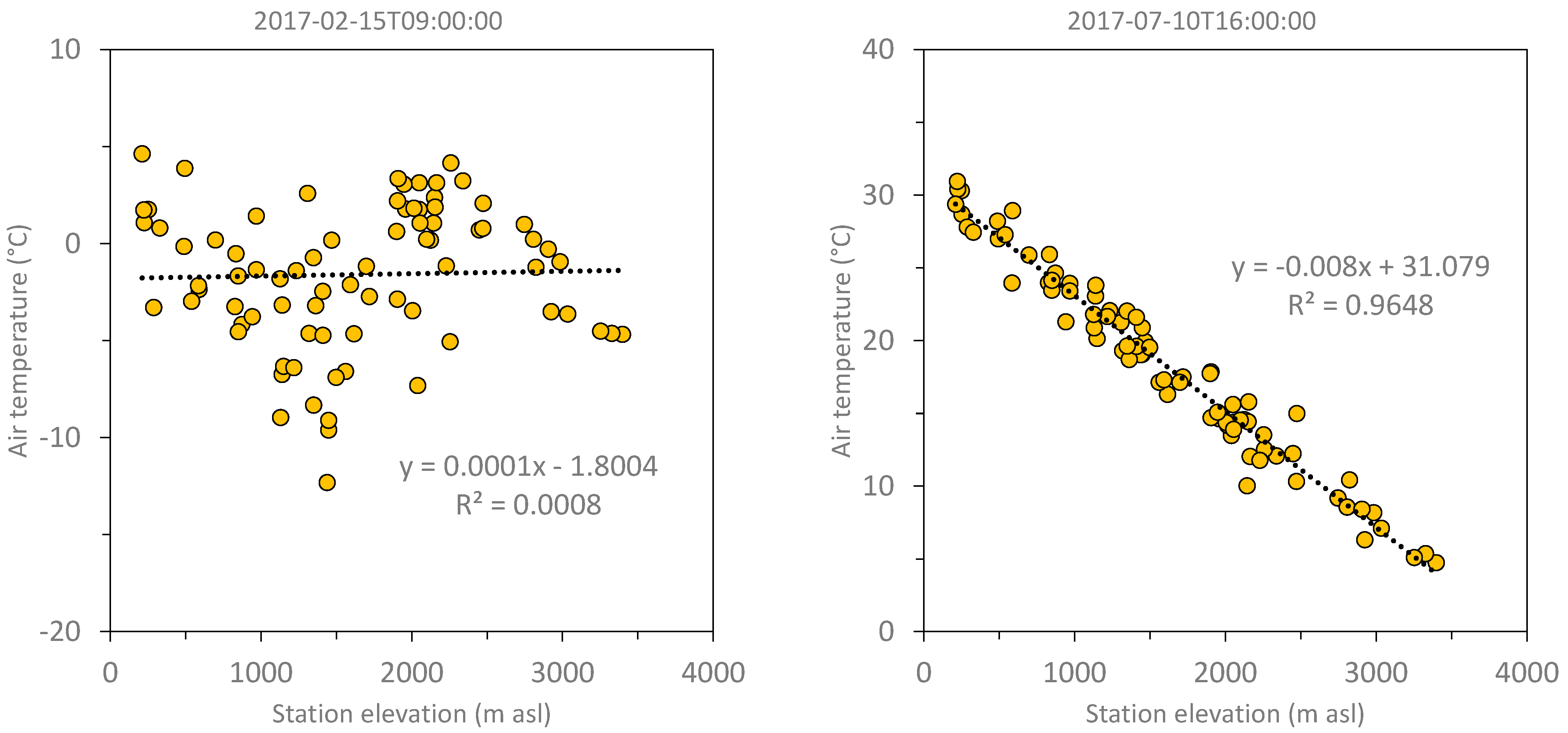
To verify the effect of the temperature lapse rate on the interpolation of the temperature data, a jackknife cross validation was applied considering the temperature measurements from 2016 to 2019. At each hour, in turn, the data measured at a station were removed and the remaining measurements were interpolated to reconstruct the removed data, iteratively for all the available stations. For each hour the root mean square error was calculated between the observed data and those reconstructed with interpolation. The procedure was repeated considering the following: the interpolation without lapse rate, the interpolation with standard lapse rate (−0.0065 °C m−1) and the interpolation with lapse rate updated hourly from the linear regression of the observed data with respect to the altitude. Figure 3 shows the averaged results on a monthly scale. Figure 3 (left) shows the monthly air temperature lapse rate computed from the linear regression of the observed data and the related R2 compared to the standard lapse rate. It is noted that only in the period April–July was the lapse rate calculated from the data comparable to the standard gradient, while the value of the calculated lapse rate decreases (in absolute value) significantly in the remaining months of the year, with a minimum in December equal to −0.0037 °C m−1. The value of the R2 of the linear regression is relatively high (>0.8) in the period between March and September, while it decreases in the rest of the year due to the thermal inversion phenomenon, frequently occurring in autumn and winter, which causes a significant deviation from the linear trend of temperature with altitude. Figure 4 shows two examples of linear regression applied to the measured data: The first is relative to 9:00 of 2017/02/15, when thermal inversion is significant and data are not linearly correlated; the second is relative to 16:00 of 2017/07/10, when the linear correlation between air temperature and station elevation is significant.

Figure 3.
Monthly air temperature lapse rate computed from linear regression of observations and related R2 compared to standard lapse rate (left) and monthly average root mean square error (RMSE) resulting from interpolation jackknife cross validation considering no lapse rate, standard lapse rate and lapse rate computed from data (right).
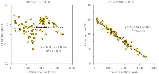
Figure 4.
Linear regression between air temperature observations and station elevation at 9:00 of 2017/02/15 (left), and at 16:00 of 2017/07/10 (right).
Figure 3 (right) shows the monthly average results of the cross validation. We note how the interpolation that updates the lapse rate at each step shows a lower error in all months compared to considering the standard lapse rate or not considering a lapse rate in the interpolation.
3.1.2. Precipitation Interpolation
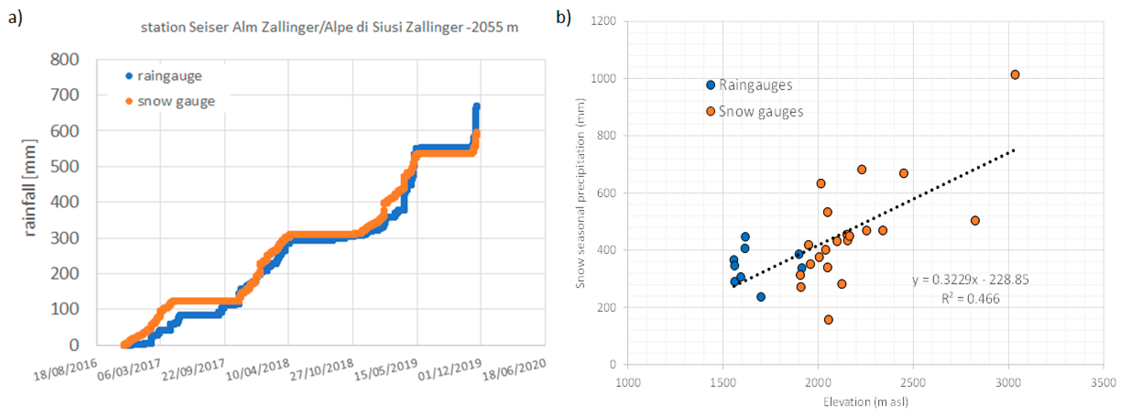
There is generally a limited number of rain gauges at high elevations due to the difficulties of installing and maintaining them. Even when there are stations, the precipitation measurement is often affected by significant errors, especially in the winter period caused by the presence of wind and by the malfunctioning of the heating system for snowfall melting. Precipitation in the Alps generally follows an increasing trend with elevation. Reconstructing a precipitation field considering only the measurements available at lower altitudes leads to an underestimation of the total precipitation volume. It is therefore crucial to evaluate the precipitation lapse rate to be used in spatial interpolation, including the measurements at the highest elevations. To compensate for the lack of rain gauges at high altitudes, measurements from snow gauges were considered in this analysis. Precipitation was calculated from the increases in height measured by the snow gauge, assuming the minimum snow density valid for newly deposited snow. The procedure was validated at the Alpe di Siusi Zallinger station, where precipitation and snow depth measurements were available at the same time. Figure 5a shows the good agreement between the cumulative precipitation measured by the rain gauge and that calculated from the snow height data, selecting the periods between November and April when, at high altitudes, due to the low air temperature, precipitation falls in the form of snow.
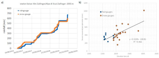
Figure 5.
Precipitation estimates from nivometric station (a) and correlation of precipitation with elevation (b).
For the calculation of the snow season lapse rate, the precipitation measurements of the stations above 1500 m with a percentage of missing data lower than 25% (9 stations) and the data of the snow gauges (21 stations), which reach an altitude of 3035 m a.s.l., were analyzed. The considered period is between 2016 and 2019. The vertical lapse rate was computed from the linear regression of snow season precipitation and station elevation (Figure 5b). The final value 0.000073 mm/h/m was subsequently used for spatial interpolation of precipitation measurements.
3.2. Snow Model Calibration and Validation against Ground and Satellite Data
At first, the snow melt parameters, Tb and Cm in Equation (4), are assumed to be, respectively, 0 °C and 4.32 mm d−1 °C−1, while Tlow and Tup are both equal to 0 °C, resulting from a previous calibration of the FEST-WB snow melt model in the Toce one in Piemonte alpine area in Italy [8].
The threshold temperature values, Tlow and Tup, depend on local meteorological conditions, so a wide range of values are available in literature, from −1 to 3 °C [61], from −1 °C to 7 °C [62] and from 0.5 °C to 1 °C [63] to a maximum value of 5.5 °C [64]. In the literature, a large variability of the melt Cm parameter value also exists, ranging from 2.7 mm d−1 °C −1 to 11.6 mm d−1 °C−1, varying from site to site related to differences in the importance of the radiation components, air temperature and wind velocity [19,64], while the parameter Tb is considered equal to 0 °C [19].
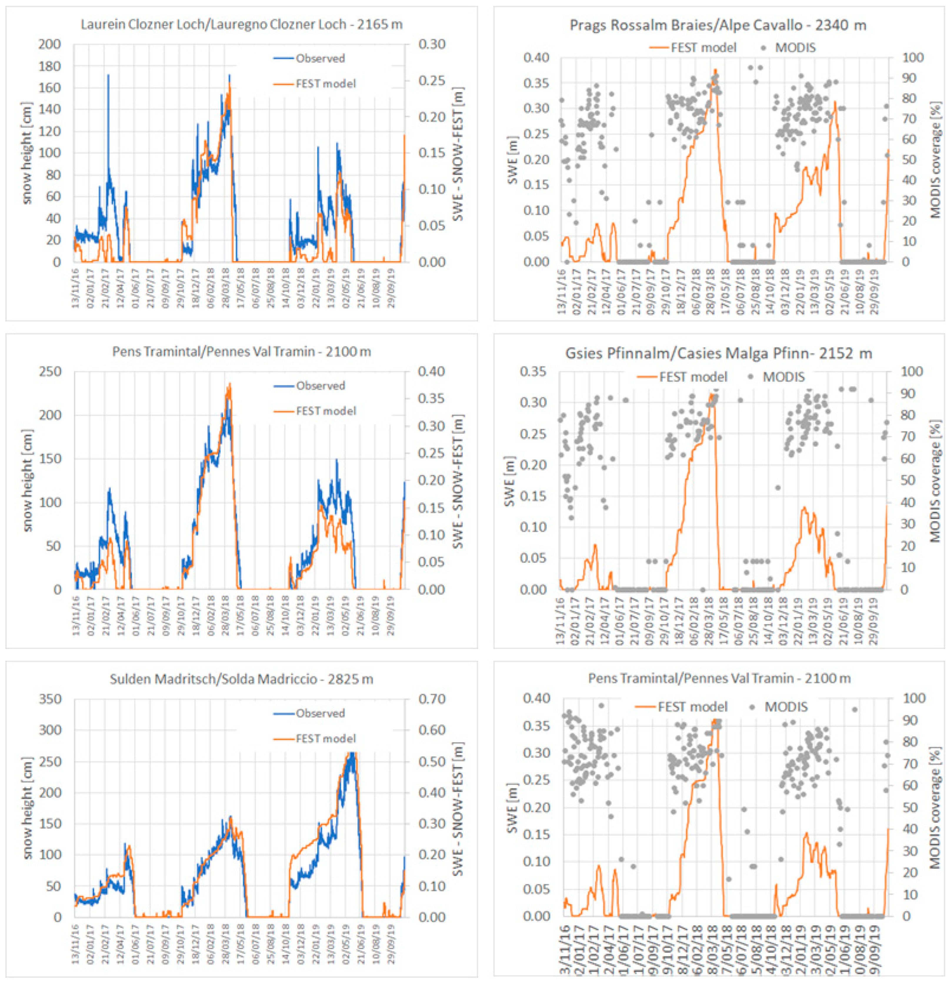
The results of the calibration based on the measured ground data are summarized in Figure 6, where the modeled snow dynamics are compared with the ground observed snow depths data for three selected stations. The comparison is performed only in terms of accumulation and melt times, as a “snow”–“no snow” series; while a direct comparison of simulated snow water equivalent and measured snow heights is not possible because the snow density is not known. In fact, we recall that the output of the FEST-EWB snow model is the snow water equivalent (e.g., which produce a direct impact on hydropower production), while it does not reproduce the complex processes of the snow pack [65]. The model generally performs well both in the accumulation and the melting period, but FEST-EWB underestimates the observed snow coverage by about 7%, globally. The months in which the major differences are registered are from June to September; this is probably due to the fact that snowfalls occurring in summer are of low intensity and thus hardly representable. This result is confirmed by the contingency tables which are build up including simulated snow data for different combination of Tup and Tlow and observed snow depth, for each single station.
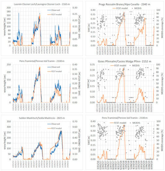
Figure 6.
FEST-EWB snow dynamics calibration against ground snow height and MODIS snow cover at the pixel of different ground stations from 2016 to 2019.
In Table 2, the mean contingency table for all 21 ground stations is reported resulting in a CPI of 92%. The values of the best fit calibrating parameters are 0 °C for Tlow, 1 °C for Tup and Cm 4.32 mm d−1 °C−1; while for snow melt, Tb is equal to 3 °C.

Table 2.
The correct performance index (CPI) for all the stations from 2016 to 2019, between FEST-EWB model and ground height and MODIS snow cover at the pixel of the ground stations.
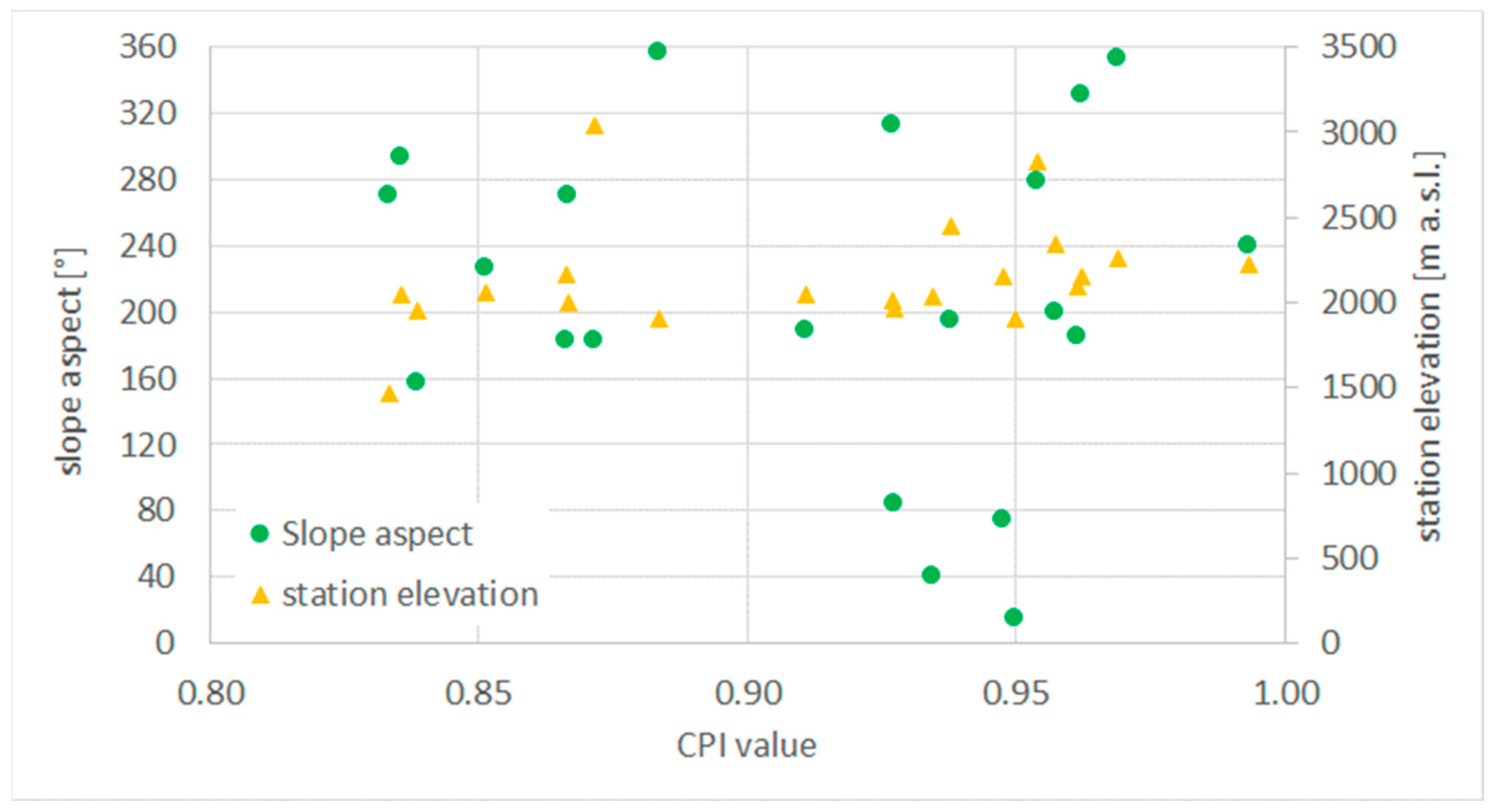
In Figure 7 the CPI values for each single station is shown in respect to station elevation and slope aspect, but no clear tendency is observable. This is of particular relevance confirming the ability of the degree-day model which doesn’t consider the solar radiation (e.g., shadowed areas).
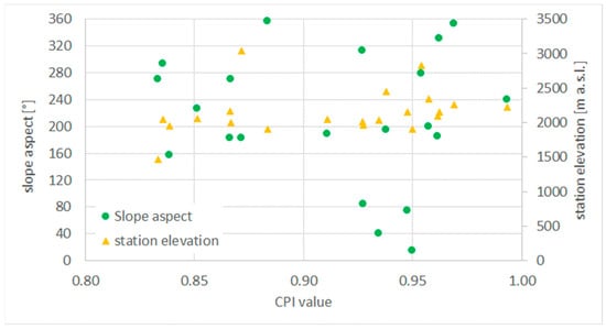
Figure 7.
CPI for each station and its variability with elevation and aspect.
The FEST-EWB snow model has then been validated against MODIS snow cover data at both the different ground stations and the whole basin area. In Figure 6, the modeled snow dynamics with the selected parameters’ configuration is reported along with MODIS data at three example stations, showing a higher variability with respect to ground information. The contingency tables are then computed for all the stations for all the cloud free days of available satellite images, and in Table 2, the mean values are reported, resulting in a CPI of 87 %.
None of the computed analyses used for calibration consider the spatial distribution of snow cover over the whole area. Hence, the model is then validated by comparing the simulated and observed maps of snow cover in each pixel of the study domain.
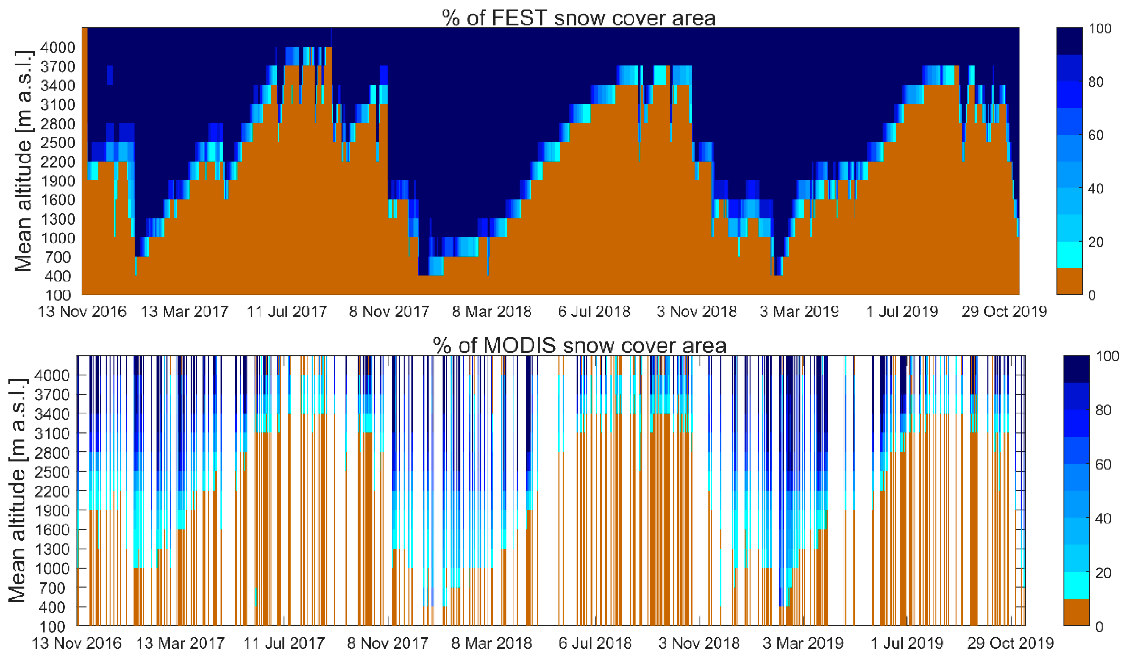
In Figure 8 the, time evolution of the snow-covered area from the MODIS and FEST-EWB models is reported for different classes of zonal elevation. Good agreement is clearly detectable from both the spatial distribution of snow at high and low altitudes and from the whole season dynamics (e.g., accumulation, winter and melt periods). It is worth noticing the several missing dates in the MODIS analysis due to the high percentage of cloud cover (higher than 40%), while the FEST-EWB model is capable of filling this information gap.
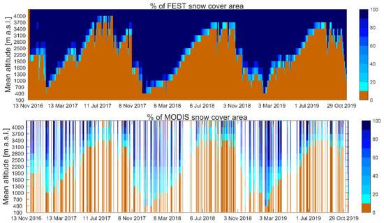
Figure 8.
FEST and MODIS snow coverage area from 2016 to 2019 divided by basin altitude.
Contingency maps are also computed for each available date to quantitatively identify the correct correspondence between modeled and observed data, grouping the agreements “snow–snow” and “no snow–no snow”, as well as the disagreements “snow MODIS–no snow FEST-EWB” and “snow FEST-EWB–no snow MODIS”. From these, the CPI index is computed, confirming the good agreement over the whole area and the seasons with a mean 89.2% and a standard deviation of 10%, which is comparable to the local stations’ analysis.
3.3. Lake Inflow Volume and Energy Production
In order to assess the water availability impacts on hydropower production, the total observed annual production is firstly compared with the annual estimated power production from precipitation. In Table 3, the differences between the estimated and observed mean annual productions are reported in terms of the relative error and the RMSE. Positive biases (e.g., estimated production higher than measured) are observable in all the hydropower plants, with errors between 16 and 25%, except for Glorenza and Lappago (−18 and −22%, respectively). These two opposite behaviors are explainable when considering, for example, the two hydropower plants of Glorenza and Lasa in more detail. The estimates at the Lasa powerplant are slightly overestimating the measured ones, which is mainly due to the fact that the summer rainfall in the Gioveretto basin can be intense, overpassing the powerplant capacity of generating energy, thus producing spillways from the dam during summer. For the Glorenza powerplant, an opposite situation is observable with the estimated annual production being lower than the measured one. This may be explained by the fact that during summer, different auxiliary intakes are activated, increasing the available water in the San Valentino basin.

Table 3.
Summary differences of observed and simulated annual production.
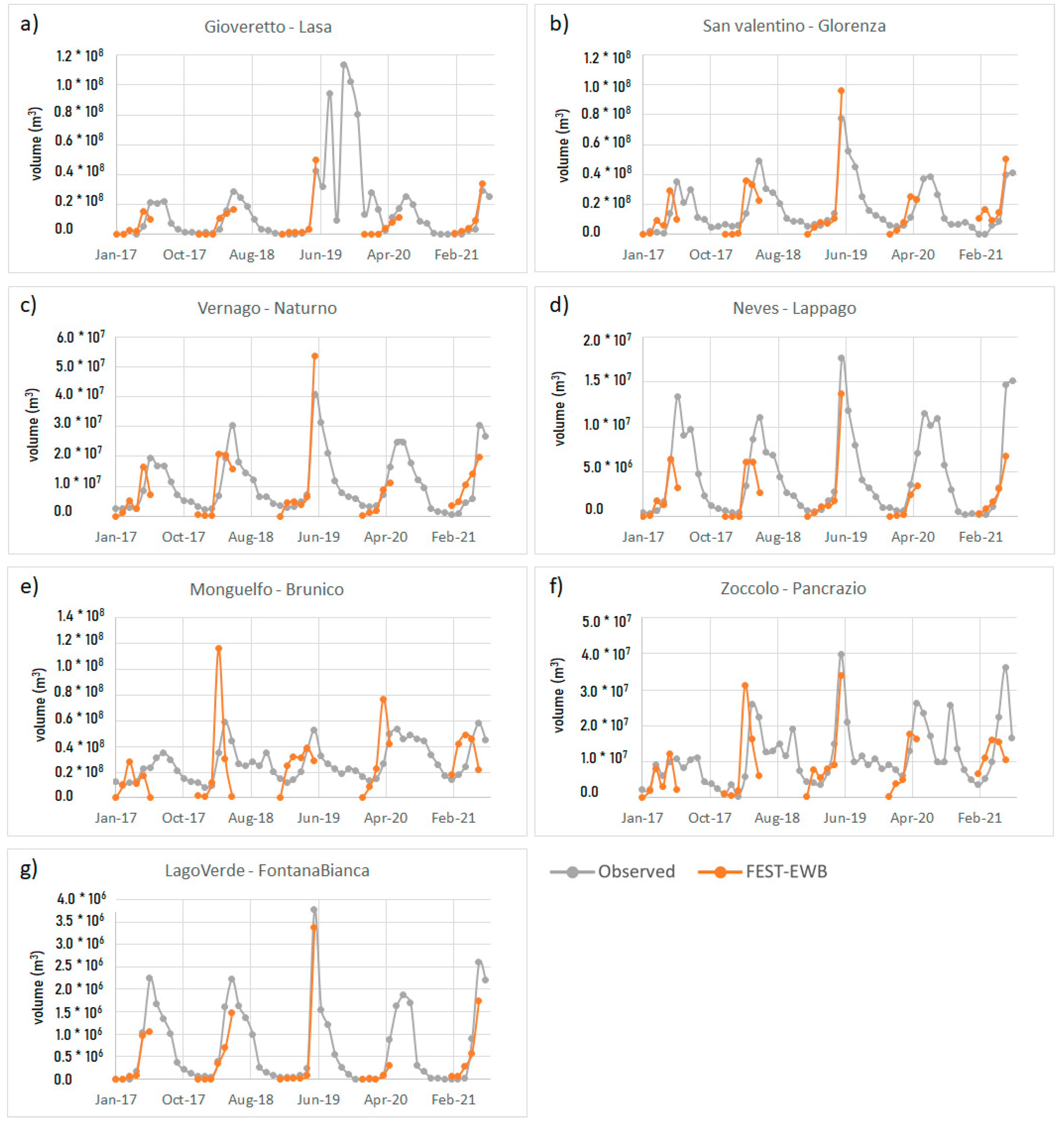
Then, to validate the FEST-EWB snow model and the entire procedure, the melt season (from March to June) is considered with almost all the power production is generated by the snow melt volume. So, the monthly inflow lake volumes from snow melt are computed from the FEST-EWB model and compared with the observed values for the different power plants from 2017 to 2021. In Figure 9, the results are shown, highlighting the agreement between the observed and modeled data, either for large catchments with high water volumes, such as the Monguelfo at Brunico power plant, or for small high elevation basins, such as Lago Verde at Fontana Bianca. Usually, the model is able to correctly reproduce the low flow values of January and February months, as well as the high values of June and July. Small discrepancies are visible for Monguelfo and for Zoccolo in some years, where a clear anticipation of the melt season is produced by the model with erroneously high values in June, which result in too low values in July. This might be related to the lower altitude of these basins in respect to the others, then having mean higher air temperatures.
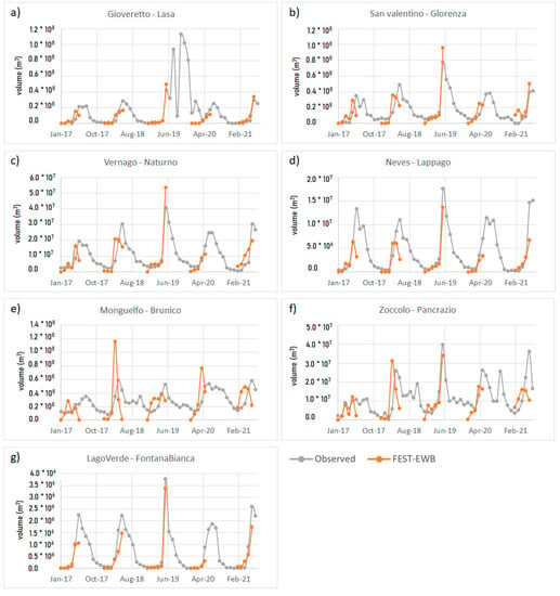
Figure 9.
Monthly lake inflow volumes for the different Hydropower plants from 2017 to 2021: (a) Lasa plant in the Gioveretto basin, (b) Glorenza plant in the San Valentino basin, (c) Naturno plant in the Vernago basin, (d) Lappago plant in the Neves basin, (e) Brunico plant in the Monguelfo basin, (f) Pancrazio plant in the Zoccolo basin, (g) Fontana Bianca plant in the Lago Verde basin.
These results are confirmed by the statistical indices of Table 4 showing low RMSE values in respect to the mean values typical of the specific basin, as well as low RRMSE values ranging between 2.5 and 3.6%. High Nash Sutcliffe index values are reported for all the basins.

Table 4.
RRMSE, RMSE and the Nash Sutcliffe index of observed and simulated data of monthly lakes inflow volumes and energy production.
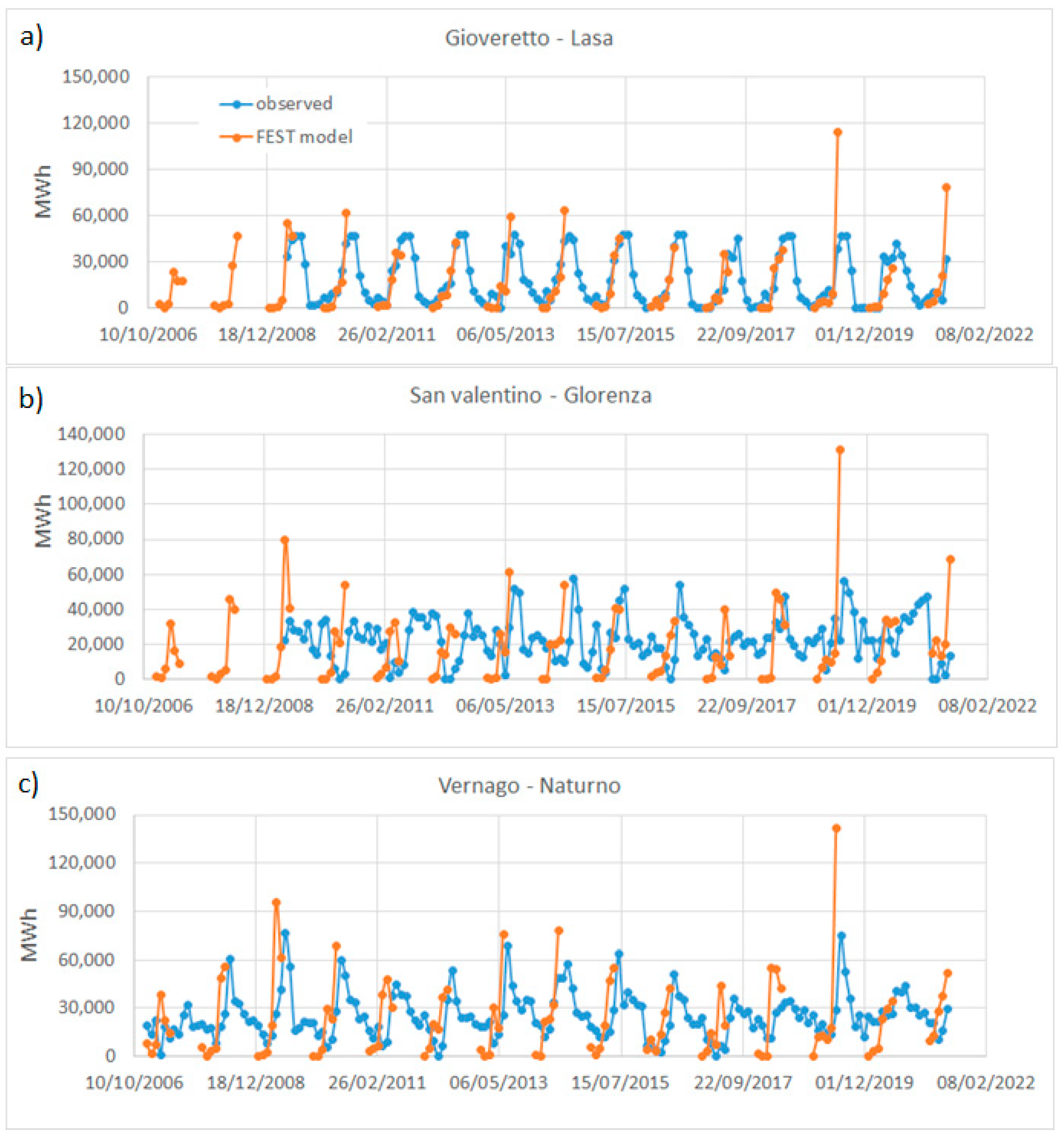
Finally, the monthly energy productions computed from the FEST-EWB model are compared to those observed values at the three available powerplants from 2006 to 2020: Naturno, Glorenza and Lasa (Figure 10). A good agreement is generally observable, especially during the first months of the melt season (March to May), while a higher variability results during the summer period. The errors are reported in Table 4 as the RRMSE and RMSE of the observed and simulated data. Glorenza and Naturno have a RMSE value of about 2.5 MWh, while a lower one is found for Lasa of around 1.5 MWh.
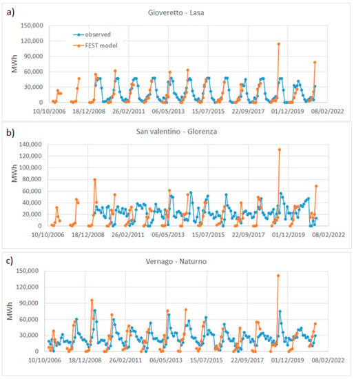
Figure 10.
Monthly energy production (MWh) for the three power plants of (a) Lasa, Glorenza (b) and Naturno (c).
With respect to the monthly lakes’ inflow volume, the energy production higher discrepancies are obtained between the observed and measured data, especially on the low and high production peaks. This might be explained by the fact that during January and February, no snow melt is observable in these high mountain basins, producing no flow. Instead, the powerplant is producing energy anyway because the lake is full of water. Conversely, during June and especially July, in addition to the snow melting, the liquid precipitation is also added, which could also be intense, giving rise to water volumes greater than the generation capacity of the power plant. The model is not considering this limitation and provides the natural potential energy production. This is clearly visible in the summer seasons of 2019 and 2021 where, for all the powerplants, an extremely high peak of potential production is visible in July.
3.4. Effect of Meteorological Forecast on SWE and Energy Production
The effect of meteorological forecasts on hydrological and energy variables is evaluated from the coupling of weather and hydrological models. The meteo-hydrological chain, set up using the ensemble meteorological outputs as inputs in the FEST-WB model, provides SWE and energy production every day with a forecast horizon of 7 days. The analyzed dataset includes 154 days of simulations from 31 January to 30 June 2020. Since the weather model has a forecast horizon of 7 days, in order to assess the forecasting chain, the statistical analysis has been carried out starting from “day+0”, i.e., the forecast at the same day of the initialization date run, up to “day+7”. This last run considers all forecast performances at 7 days from the initialization date.
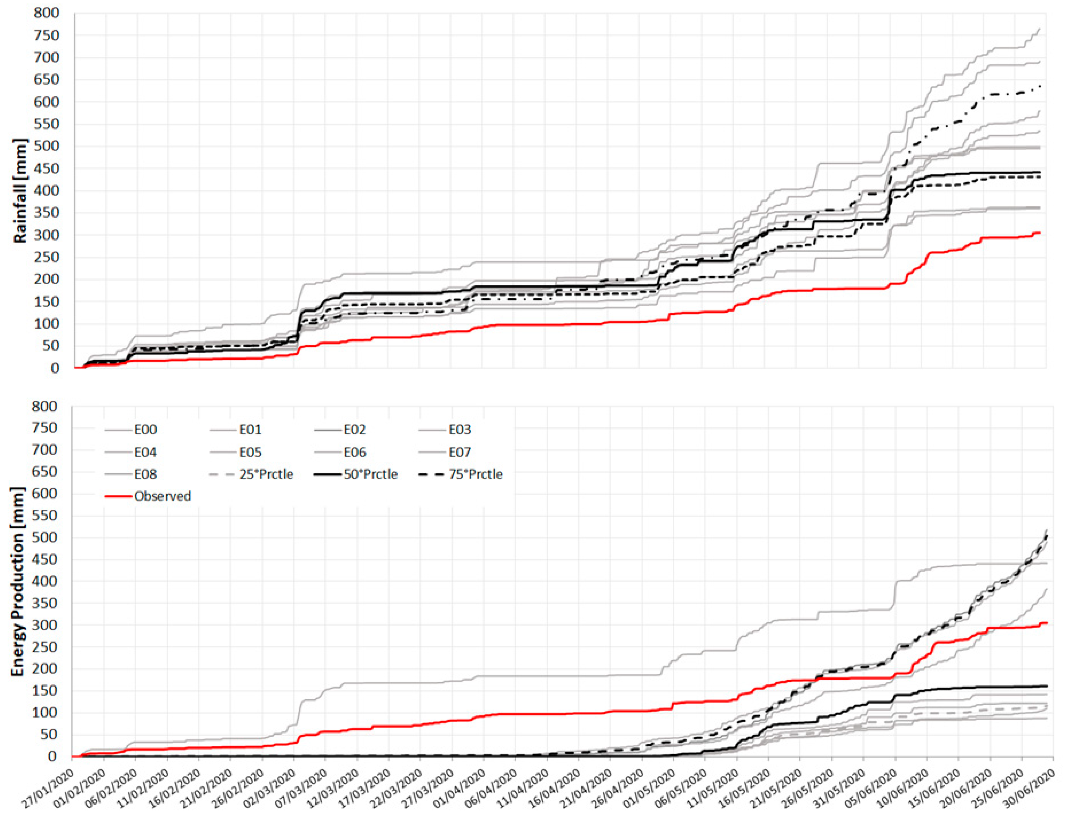
In Figure 11, the cumulated hourly precipitation and energy production are shown at day+1 forecast for the whole period, for example, for the Gioveretto basin. In details, the model simulation forced with observed data and the forecasted variables, respectively, by the WRF ensembles, plus the 25th, 50th and 75th percentiles are reported. The precipitation forecast shows a sensible overestimation compared to the observed weather data, being in the 50th percentiles greater than the observed data of 200 mm over 5 months. This issue may be related to both the accuracy of ground precipitation data interpolation for high elevation areas as well as the ability of the weather forecast model to catch the dynamics over mountainous areas. The hydrological variable of energy production, as rainfall plus melting, displays a considerable overestimation 50th percentiles greater, about 170 mm, over the 5 analyzed months.
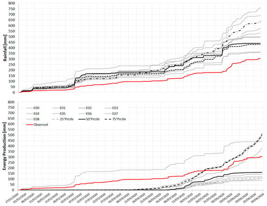
Figure 11.
The cumulated hourly precipitation (upper plot) and energy production (lower plot) at day +1 forecast from 31 January to 30 June 2020 for the Gioveretto basin. The red line shows: the observed precipitation data and the FEST-EWB model simulation forced with observed data for energy production, the 9 colored lines display the forecasted variables respectively by the WRF ensembles, while the black line is the median and the black dotted lines the 25th, 75th percentiles.
In Figure 12, the results of the meteo-hydrological forecast skills are summarized for all catchments and all analyzed variables in terms of Mean Absolute Error (MAE) between the WRF 50th ensemble percentile and the FEST-EWB estimates for six forecast lead times (from day 0 to day+6). The minimum MAE value is shown in blue color, while the dark red corresponds to the maximum MAE. In particular, the considered variables are air temperature, precipitation, energy production, snow melt and SWE.

Figure 12.
Mean Absolute Error (MAE) between the WRF esemble 50th Percentile and FEST-EWB estimates for six forecast lead times.
The forecast performances are extremely variable across the basins due to the highly irregular topography and mainly according to their mean elevation and their location. Indeed, performances are generally more reliable for the lead time day+1 and, in particular, for the first days of the forecast horizon and decrease in the later forecast days. In particular, rainfall MAE is generally very low for the first two days of forecasts and then increase, except for the two basins, Neves and San Valentino, which show higher MAE values. These two basins are located in the north part of the case study areas and on the southern side of the mountains. Air temperature forecasts follow a more regular behavior with low MAE values for day 0 and day+1 increasing with the increase in the lead time in all the analyzed catchments. These meteorological variables errors are then reflected into the hydrological forecasts reporting snow melt MAE values, which decrease with the lead time in some catchments while for others, remain almost constant. High MAE values are found for the two basins Neves and San Valentino (e.g., high rainfall MAE), as well as Gioveretto and Vernago, which show higher MAE values in air temperature after day+3. Variable MAE values are obtained for energy production with no precise trend on the skills of the meteorological forecasts. The highest values are again observable for the two Neves and San Valentino basins. The SWE variable is instead characterized by a less variable behavior among the basins with an MAE value which decreases with the forecast horizon in a similar way, even though higher values are found in the Neves catchment.
4. Discussion and Conclusions
In this paper, we presented a system for supporting the hydropower production for eight small river basins underlying a hydroelectric power plant in the Italian Alps in the Province of Bolzano. This is an area with typical Alpine characteristics, that may impact the system with specific issues related to high altitude, morphological features and harshness of the mountainous environment in general.
One limitation of the presented system is that it requires real time detailed precipitation and temperature data in order to perform snow mass balance and provide melting amount. To this purpose, some methods have been developed and tested in order to get the maximum from available data, thus providing reliable output. These methods are not specific of the investigated area and can be applied in any mountainous environment.
The system reliability depends on the accuracy of three components: spatial interpolation of meteorological observations, a mathematical model and quantitative meteorological forecasts.
A common problem at higher elevations is the shortage of precipitation measurement. As a matter of fact, the number of rain gauges at high elevations is generally very limited and, when available, data are often affected by significant errors caused by wind and by the malfunctioning of the heating system for snowfall melting. In this paper, a methodology to compensate for the lack of rain gauges at high altitudes, by using measurements from snow gauges, has been validated. Precipitation was calculated from snow gauge measurements assuming the minimum snow density for newly deposited snow. By merging data coming from snow gauges at higher altitude and precipitation acquired by rain gauges at lower altitude, vertical precipitation lapse rate was computed from the linear regression of measurements and station elevation. The advantage of this method is that snow gauge data are not required for real time application. Data from snow gauges are used in offline analysis only to assess the vertical lapse rate to be used for real time interpolation of data from rain gauges. An indirect check of the method for precipitation interpolation comes from the comparison of the total observed annual production with the annual estimated power production from precipitation. The latter represents the potential power production and should be greater or equal to energy production. If this is not the case, the error would be due to precipitation underestimation.
A second investigated point is the interpolation of air temperature data. Indeed, air temperature is strongly affected by topography, and lapse rate may be driven by local morphological properties and seasonal variability. A procedure was implemented to compute the air temperature vertical lapse rate for each hour based on the linear regression of air temperature measurements and station elevation. A jackknife validation demonstrated the advantages of this procedure with respect to considering a standard constant lapse rate or not considering lapse rate at all. The RMSE keeps below 2 °C when the lapse rate is updated hourly, it increases above 3 °C during winter when a standard constant value is used and ranges between 4 °C and 5 °C when no lapse rate is used.
As far as the accuracy of mathematical simulation is concerned, the snow module parameters of the FEST-EWB model have been calibrated by comparing snow depth measurements to modelled snow water equivalents and validated against MODIS snow coverage maps. Despite that snow water equivalents cannot be directly compared to snow depths and MODIS data, the model accuracy can be assessed in reproducing time series of “snow” and “no snow” status. On the other hand, the aim of the simulation is far from reproducing the complex processes the snow pack is subjected to, after snow deposition. The model generally performs well both in accumulation and melting period with CPI about 0.9 (0.92 against snow gauges data, 0.87 against MODIS data). The shortage of available measurements did not allow us to perform model validation. However, model validity to simulate the spatial distribution of snow coverage has been assessed by comparing the simulated and observed maps of snow cover in each pixel of the study domain, with quite satisfactory results.
A further step toward model validation implied the comparison of model output to two available datasets: the monthly inflow lake volumes from 2017 to 2021 for most of the powerplants and the monthly energy productions available only for the three powerplants, Naturno, Glorenza and Lasa, from 2006 to 2020. From the comparison to lake inflow volumes, the results show an agreement between the observed and modeled data, either for large catchments, such as Monguelfo at the Brunico power plant, and for small high elevation basins, such as Lago Verde at Fontana Bianca. Anticipation of the melt season was found in Monguelfo and Zoccolo in some years. This might be related to the lower altitude of these basins, thus having higher air temperatures. Further analysis to calibrate spatially distributed snow melt parameter is being carried out in order to improve model performance at low elevation basins.
From comparison to energy production, good agreement is generally achieved, especially during the first months of the melt season (March to May), while higher variability is obtained during the summer period.
A final analysis implies the use of WRF-ARW meteorological forecasts to assess the system capability of forecasting the snow melt amount on a horizon of 7 days. To improve forecast quality, an ensemble configuration with nine instances is used, each with a different physical configuration and with a different set of initial and boundary conditions. Precipitation forecasts show a sensible overestimation compared to observed weather data, which reflects the general overestimation of forecasted energy production. In terms of skill scores, the opposite behavior is found for precipitation MAE that increases with lead time, except for San Valentino and Neves where MAE is greater in the first days. The SWE variable is characterized by a less variable behavior among the basins with a MAE value, which decreases with the forecast horizon. Energy production, being affected by the variability of all other variables, does not show a general trend of MAE, with greater values for Neves and San Valentino basins.
The procedures presented in this paper validated on Alpine area, can be generalized to any other mountainous area where an estimation of current and forecasted snow water equivalent and melting amount are required.
Author Contributions
Conceptualization, C.C., G.R. and A.P.; methodology, C.C., G.R., A.P., M.M., R.S., G.L. (Giulio Lanzingher); software, C.C., G.R., A.P. and G.L. (Gabriele Lombardi); formal analysis, C.C., G.R. and A.P.; data curation, M.Q., G.L. (Gabriele Lombardi), G.L. (Giulio Lanzingher); writing—original draft preparation, C.C.; writing—review and editing, C.C., G.R., A.P., G.L. (Gabriele Lombardi) and R.S. All authors have read and agreed to the published version of the manuscript.
Funding
This research was partially funded by Alperia Greenpower Srl.
Conflicts of Interest
The authors declare no conflict of interest. The Funder contributed in the design of the study and data collection and interpretation.
References
- Kaygusuz, K. Hydropower and the world’s energy future. Energy Sources 2004, 26, 215–224. [Google Scholar] [CrossRef]
- Schaefli, B. Projecting hydropower production under future climates: A guide for decision-makers and modelers to interpret and design climate change impact assessments. Water 2015, 2, 271–289. [Google Scholar] [CrossRef] [Green Version]
- Gaudard, L.; Romerio, F. The future of hydropower in Europe: Interconnecting climate, markets and policies. Environ. Sci. Policy 2014, 37, 172–181. [Google Scholar] [CrossRef]
- Gaudard, L.; Romerio, F.; Valle, D.F.; Gorret, R.; Maran, S.; Ravazzani, G.; Stoffel, M.; Volonterio, M. Climate change impacts on hydropower in the Swiss and Italian Alps. Sci. Total Environ. 2014, 493, 1211–1221. [Google Scholar] [CrossRef]
- Ravazzani, G.; Dalla Valle, F.; Gaudard, L.; Mendlik, T.; Gobiet, A.; Mancini, M. Assessing climate impacts on hydropower production: The case of the toce river basin. Climate 2016, 4, 16. [Google Scholar] [CrossRef]
- Beniston, M.; Stoffel, M.; Hill, M. Impacts of climatic change on water and natural hazards in the alps: Can current water governance cope with future challenges? examples from the European ACQWA project. Environ. Sci. Policy 2011, 14, 734–743. [Google Scholar] [CrossRef] [Green Version]
- Bongio, M.; Avanzi, F.; De Michele, C. Hydroelectric power generation in an Alpine basin: Future water-energy scenarios in a run-of-the-river plant. Adv. Water Resour. 2016, 94, 318–331. [Google Scholar] [CrossRef]
- Corbari, C.; Ravazzani, G.; Martinelli, J.; Mancini, M. Elevation based correction of snow coverage retrieved from satellite images to improve model calibration. Hydrol. Earth Syst. Sci. 2009, 13, 639–649. [Google Scholar] [CrossRef] [Green Version]
- Magnusson, J.; Wever, N.; Essery, R.; Helbig, N.; Winstral, A.; Jonas, T. Evaluating snow models with varying process representations for hydrological applications. Water Resour. Res. 2015, 51, 2707–2723. [Google Scholar] [CrossRef] [Green Version]
- Verbunt, M.; Gurtz, J.; Jasper, K.; Lang, H.; Warmerdam, P.; Zappa, M. The hydrological role of snow and glaciers in alpine river basins and their distributed modelling. J. Hydrol. 2003, 282, 36–55. [Google Scholar] [CrossRef]
- Shamir, E.; Georgakakos, K.P. Distributed snow accumulation and ablation modelling in the American River basin. Adv. Water Resour. 2006, 29, 558–570. [Google Scholar] [CrossRef]
- Adam, J.C.; Lettenmaier, D.P. Adjustment of global gridded precipitation for systematic bias. J. Geophys. Res. 2003, 108, 4257. [Google Scholar] [CrossRef]
- Avanzi, F.; Ercolani, G.; Gabellani, S.; Cremonese, E.; Pogliotti, P.; Filippa, G.; Morra di Cella, U.; Ratto, S.; Stevenin, H.; Cauduro, M.; et al. Learning about precipitation lapse rates from snow course data improves water balance modeling. Hydrol. Earth Syst. Sci. 2021, 25, 2109–2131. [Google Scholar] [CrossRef]
- Bocchiola, D.; Rosso, R. The distribution of daily snow water equivalent in the central Italian Alps. Adv. Water Resour. 2007, 30, 135–147. [Google Scholar] [CrossRef]
- Gelfan, A.N.; Pomeroy, J.W.; Kuchment, L.S. Modeling Forest Cover Influences on Snow Accumulation, Sublimation, and Melt. J. Hydrometeor. 2004, 5, 785–803. [Google Scholar] [CrossRef]
- Rango, A.; Martinec, J. Application of a snowmelt–runoff model using Landsat data. Nord. Hydrol. 1979, 10, 225–238. [Google Scholar] [CrossRef]
- Mazurkiewicz, A.B.; Callery, D.G.; McDonnell, J.J. Assessing the controls of the snow energy balance and water available for runoff in a rain-on-snow environment. J. Hydrol. 2008, 354, 1–14. [Google Scholar] [CrossRef]
- Howard, C. Revisiting the degree-day method for snowmelt computations-Discussion. Water Resour. Bull. 1996, 32, 411–413. [Google Scholar] [CrossRef]
- Hock, R. Temperature index melt modelling in mountain areas. J. Hydrol. 2003, 282, 104–115. [Google Scholar] [CrossRef]
- He, Z.H.; Parajka, J.; Tian, F.Q.; Blöschl, G. Estimating degree-day factors from MODIS for snowmelt runoff modeling. Hydrol. Earth Syst. Sci. 2014, 18, 4773–4789. [Google Scholar] [CrossRef] [Green Version]
- Bormann, K.J.; Evans, J.P.; McCabe, M.F. Constraining snowmelt in a temperature-index model using simulated snow densities. J. Hydrol. 2014, 517, 652–667. [Google Scholar] [CrossRef]
- Marsh, C.B.; Pomeroy, J.W.; Spiteri, R.J. Implications of mountain shading on calculating energy for snowmelt using unstructured triangular meshes. Hydrol. Process. 2012, 26, 1767–1778. [Google Scholar] [CrossRef] [Green Version]
- Rango, A.; Martinec, J. Revisting the degree-day method for snowmelt computations. Water Resour. Bull. 1995, 31, 657–669. [Google Scholar] [CrossRef]
- Singh, P.; Kumar, N. Determination of snowmelt factor in the Himalayan region. Hydrol. Sci. J. 1996, 41, 301–310. [Google Scholar] [CrossRef]
- Immerzeel, W.W.; Droogers, P.; de Jong, S.M.; Bierkens, M.F.P. Large-scale monitoring of snow cover and runoff simulation in Himalayan river basins using remote sensing. Remote. Sens. Environ. 2009, 113, 40–49. [Google Scholar] [CrossRef]
- Franz, K.J.; Karsten, L.R. Calibration of a distributed snow model using MODIS snow covered area data. J. Hydrol. 2013, 494, 160–175. [Google Scholar] [CrossRef]
- Parajka, J.; Blöschl, G. The value of MODIS snow cover data in validating and calibrating conceptual hydrologic models. J. Hydrol. 2008, 358, 240–258. [Google Scholar] [CrossRef]
- Magnusson, J.; Nævdal, G.; Matt, F.; Burkhart, J.F.; Winstral, A. Improving hydropower inflow forecasts by assimilating snow data. Hydrol. Res. 2020, 51, 226–237. [Google Scholar] [CrossRef]
- Largeron, C.; Dumont, M.; Morin, S.; Boone, A.; Lafaysse, M.; Metref, S.; Cosme, E.; Jonas, T.; Winstral, A.; Margulis, S. Toward Snow Cover Estimation in Mountainous Areas Using Modern Data Assimilation Methods: A Review. Front. Earth Sci. 2020, 8, 325. [Google Scholar] [CrossRef]
- Parajka, J.; Blöschl, G. Spatio-temporal combination of MODIS images-potential for snow cover mapping. Water Resour. Res. 2008, 44. [Google Scholar] [CrossRef]
- Da Ronco, P.; De Michele, C. Cloud obstruction and snow cover in Alpine areas from MODIS products. Hydrol. Earth Syst. Sci. 2014, 18, 4579–4600. [Google Scholar] [CrossRef] [Green Version]
- Li, D.; Lettenmaier, D.P.; Margulis, S.A.; Andreadis, K. The Value of Accurate High-Resolution and Spatially Continuous Snow Information to Streamflow Forecasts. J. Hydrometeorol. 2019, 20, 731–749. [Google Scholar] [CrossRef]
- Jörg-Hess, S.; Griessinger, N.; Zappa, M. Probabilistic Forecasts of Snow Water Equivalent and Runoff in Mountainous Areas. J. Hydrometeorol. 2015, 16, 2169–2186. [Google Scholar] [CrossRef]
- Blumen, W. Atmospheric Processes Over Complex Terrain; Meteorological Monographs 23.45; American Meteorological Society: Boston, MA, USA, 1990. [Google Scholar]
- Faccani, C.; Ferretti, R.; Visconti, G. High-Resolution Weather Forecasting over Complex Orography: Sensitivity to the Assimilation of Conventional Data. Mon. Weather Rev. 2000, 131, 136–154. [Google Scholar] [CrossRef]
- Berg, A.A.; Mulroy, K.A. Streamflow predictability in the Saskatchewan/Nelson River basin given macroscale estimates of the initial soil moisture status. Hydrol. Sci. 2006, 51, 642–654. [Google Scholar] [CrossRef] [Green Version]
- Ramos, M.H.; van Andel, S.J.; Pappenberger, F. Do probabilistic forecasts lead to better decisions? Hydrol. Earth Syst. Sci. 2013, 17, 2219–2232. [Google Scholar] [CrossRef] [Green Version]
- Dale, M.; Wicks, J.; Mylne, K.; Pappenberger, F.; Laeger, S.; Taylor, S. Probabilistic flood forecasting and decision-making: An innovative risk-based approach. Nat. Hazards 2014, 70, 159–172. [Google Scholar] [CrossRef]
- Boscarello, L.; Ravazzani, G.; Rabuffetti, D.; Mancini, M. Integrating glaciers raster-based modelling in large catchments hydrological balance: The Rhone case study. Hydrol. Process. 2012, 28, 496–508. [Google Scholar] [CrossRef] [Green Version]
- Powers, J.G.; Klemp, J.B.; Skamarock, W.C.; Davis, C.A.; Dudhia, J.; Gill, D.O.; Coen, J.L.; Gochis, D.J.; Ahmadov, R.; Peckham, S.E.; et al. The Weather Research and Forecasting Model: Overview, System Efforts, and Future Directions. Bull. Am. Meteorol. Soc. 2017, 98, 1717–1737. [Google Scholar] [CrossRef]
- Tuo, Y.; Duan, Z.; Disse, M.; Chiogna, G. Evaluation of precipitation input for SWAT modeling in Alpine catchment: A case study in the Adige river basin (Italy). Sci. Total Environ. 2016, 573, 66–82. [Google Scholar] [CrossRef] [PubMed] [Green Version]
- Mallucci, S.; Majone, B.; Bellin, A. Detection and attribution of hydrological changes in a large Alpine river basin. J. Hydrol. 2019, 575, 1214–1229. [Google Scholar] [CrossRef]
- Hall, D.K.; Riggs, G.A.; Salomonson, V.V.; Barton, J.S.; Casey, K.; Chien, J.Y.L.; Di Girolamo, N.E.; Klein, A.G.; Powell, H.W.; Tait, A.B. Algorithm Theoretical Basis Document (ATBD) for the MODIS Snow and Sea Ice-Mapping Algorithms. NASA GSFC, 2001; pp. 1–45. Available online: http://www.modis-snow-ice.gsfc.nasa.gov/atbd01.html (accessed on 11 June 2019).
- Hall, D.K.; Riggs, G.A.; Salomonson, V.V.; DiGirolamo, N.E.; Bayr, K.J. MODIS snow cover products. Remote Sens. Environ. 2002, 83, 181–194. [Google Scholar] [CrossRef] [Green Version]
- Corbari, C.; Mancini, M. Calibration and validation of a distributed energy water balance model using satellite data of land surface temperature and ground discharge measurements. J. Hydrometeor. 2014, 15, 376–392. [Google Scholar] [CrossRef]
- Corbari, C.; Huber, C.; Yesou, H.; Huang, Y.; Su, Z.; Mancini, M. Multi-Satellite Data of Land Surface Temperature, Lakes Area, and Water Level for Hydrological Model Calibration and Validation in the Yangtze River Basin. Water 2019, 11, 2621. [Google Scholar] [CrossRef] [Green Version]
- Tarboton, D.G. Measurement and modeling of snow energy balance and sublimation from snow. In Proceedings of the International Snow Science Workshop, Snowbird, UT, USA, 31 October–2 November 1994. Utah Water Research Laboratory working paper no. WP-94-HWR-DGT/00. [Google Scholar]
- Mason, S.J.; Graham, N.E. Conditional Probabilities, Relative Operating Characteristics, and Relative Operating Levels. Weather Forecast. 1999, 14, 713–725. [Google Scholar] [CrossRef]
- Skamarock, W.C.; Klemp, J.B.; Dudhia, J.; Gill, D.O.; Barker, D.; Duda, M.G.; Huang, X.-Y.; Wang, W.; Powers, J.G. A Description of the Advanced Research; WRF Version 3 NCAR Technical Note NCAR/TN-475+STR; University Corporation for Atmospheric Research: Boulder, CO, USA, 2008; p. 113. [Google Scholar] [CrossRef]
- Pielke, R.A.S.; Marland, G.; Betts, R.A.; Chase, T.N.; Eastman, J.L.; Niles, J.O.; Niyogi, D.D.S.; Running, S.W. The influence of land-use change and landscape dynamics on the climate system-relevance to climate change policy beyond the radiative effect of greenhouse gases. Philos. Trans. R. Soc. Lond. Ser. A 2002, 360, 1705–1719. [Google Scholar] [CrossRef]
- Arakawa, A.; Lamb, V.R. Computational Design of the Basic Dynamical Process of the UCLA General Circulation Model. Methods Comput. Phys. 1977, 17, 173–265. [Google Scholar]
- Lorenz, E.N. Deterministic Nonperiodic Flow. J. Atmos. Sci. 1963, 20, 130–141. [Google Scholar] [CrossRef] [Green Version]
- Leutbecher, M.; Palmer, T.N. Ensemble forecasting. J. Comp. Phys. 2008, 227, 3515–3539. [Google Scholar] [CrossRef]
- Ehrendorfer, M. Predicting the uncertainty of numerical weather forecasts: A review. Meteorol. Z. 1997, 6, 147–183. [Google Scholar] [CrossRef]
- Buizza, R.; Milleer, M.; Palmer, T.N. Stochastic representation of model uncertainties in the ECMWF ensemble prediction system. Quart. J. R. Meteorol. Soc. 1999, 125, 2887–2908. [Google Scholar] [CrossRef]
- Duan, W.S.; Huo, Z.H. An approach to generating mutually independent initial perturbations for ensemble forecasts: Orthogonal conditional nonlinear optimal perturbations. J. Atmos. Sci. 2016, 73, 997–1014. [Google Scholar] [CrossRef]
- Houtekamer, P.L.; Derome, J. Methods for ensemble prediction. Mon. Weather Rev. 1995, 123, 2181–2196. [Google Scholar] [CrossRef] [Green Version]
- Wang, X.G.; Bishop, C.H. A comparison of breeding and ensemble transform Kalman filter ensemble forecast schemes. J. Atmos. Sci. 2003, 60, 1140–1158. [Google Scholar] [CrossRef]
- Wei, M.Z.; Toth, Z.; Wobus, R.; Zhu, Y.J. Initial perturbations based on the ensemble transform (ET) technique in the NCEP global operational forecast system. Tellus A. 2008, 60, 62–79. [Google Scholar] [CrossRef] [Green Version]
- Toth, Z.; Kalnay, E. Ensemble forecasting at NCEP and the breeding method. Mon. Weather Rev. 1997, 125, 3297–3319. [Google Scholar] [CrossRef]
- Tarboton, D.G.; Luce, C.H. Utah Energy Balance Snow Accumulation and Melt Model (UEB), Computer Model Technical Description and Users Guide; Utah Water Res. Lab.: Logan, UT, USA, 1996. [Google Scholar]
- Braun, L.N. Modeling the snow-water equivalent in the mountain environment. IAHS Publ. 1991, 205, 3–17. [Google Scholar]
- US Army Corps of Engineers. Snow Hydrology: Summary Report of the Snow Investigations; Technical Report No. 1985283; North Pacific Division, Corps of Engineers, U.S. Army: Portland, OR, USA, 1956; p. 437. [Google Scholar]
- Martinec, J.; Rango, A. Parameter values for snowmelt runoff modelling. J. Hydrol. 1986, 84, 197–219. [Google Scholar] [CrossRef]
- Essery, R.; Martin, E.; Douville, H.; Fernandez, A.; Brun, E. A comparison of four snow models using observations from an alpine site. Clim. Dyn. 1999, 15, 583–593. [Google Scholar] [CrossRef]
Publisher’s Note: MDPI stays neutral with regard to jurisdictional claims in published maps and institutional affiliations. |
© 2022 by the authors. Licensee MDPI, Basel, Switzerland. This article is an open access article distributed under the terms and conditions of the Creative Commons Attribution (CC BY) license (https://creativecommons.org/licenses/by/4.0/).

