Abstract
Aquatic vegetation plays a critical role in aquatic environments and provides various valuable services. To characterize vegetation, vegetation density and flexibility are usually used as parameters, but aquatic vegetation found in nature may have a non-uniform distribution of density in the vertical direction. Studies have shown that this non-uniformity could impact the flow structure and flow resistance. With the aim of studying the effect of vertical variation of submerged vegetation density on the flow resistance and bulk flow characteristics, the hydrodynamics of three types of wooden model vegetation elements were compared in the laboratory. Vegetation models had the same density but different vertical distributions of density. All other influential parameters were kept constant so that any differences in the flow structure and the flow resistance would be attributable to the distribution of density in the vertical direction. The results show that the vertical distribution of submerged vegetation density impacts the flow field, bed shear stress, and flow resistance. There was a 41% difference in the value of the drag coefficient produced by the models. The distance between the bed and the geometrical center of vegetation elements was introduced as a parameter to quantify the effect of the vertical distribution of vegetation. There is a direct relation between this parameter with both the drag and Manning’s coefficients. The findings of this can study help researchers and practitioners use relevant vegetation parameters.
1. Introduction
Aquatic vegetation plays a crucial role in rivers, wetlands, and coastal systems, altering morphological and biogeochemical processes as well as the hydraulic functioning of these systems. Through this alteration, aquatic vegetation provides various valuable services, such as water quality improvement, coastal protection, erosion control, and habitat provision [1,2,3,4].
To incorporate aquatic vegetation within hydrodynamic models, two main approaches were employed. One approach was to model the vegetation directly in the geometry and meshing of numerical models, and the other was to either add a source term in the momentum equation in 2D/3D models or treat vegetation as roughness, which is appropriate for 1D models [5,6]. Modeling vegetation directly is computationally expensive. Therefore, the second approach is usually preferred. Source term treatment requires a model that predicts the drag force, and roughness treatment employs a model that predicts a friction coefficient, where the Manning’s coefficient is usually used. These models are generally referred to as vegetation resistance models.
Various analytical and empirical models have been developed predicting the vegetative resistance based on geometrical and biomechanical properties of vegetation and flow conditions. Specifically, vegetative resistance has been found to be a function of vegetation characteristics such as density, flexibility, distribution of the vegetation patches, flow conditions, incident flow velocity, relative submergence (flow depth to the vegetation height), etc. [7,8,9]. Most models, however, use only vegetation density, flexibility, and relative submergence as input parameters in the determination of vegetative resistance [8,10]. Moreover, most laboratory studies use rigid or flexible dowels as surrogates for real vegetation [6]. These surrogates fail to capture the morphological complexities of real vegetation and it has been shown that natural vegetation leads to more complex flow structures and turbulent characteristics [11,12,13]. Therefore, there has been debate on how detailed the morphological characterization of vegetation should be for a specific purpose of study [1,7,10].
Natural aquatic plants may have various morphological and biomechanical characteristics and vegetation density may not be uniformly distributed in the vertical direction and this non-uniformity has been shown to affect the flow characteristics. Most research studies exploring this effect have been conducted to study wave-vegetation interaction. Wu and Cox (2016) compared two patches of emergent vegetation with the different vertical distributions of density in the laboratory and found that non-uniform density distribution in the vertical direction significantly impacts the drag coefficient and wave attenuation capability of vegetation [14]. Using model vegetation in the laboratory, He et al., (2019) showed that the vertical posture of plants affects the wave dissipation coefficient [15]. Several other studies also show that vertical non-uniformity of vegetation affects wave attenuation and the flow structure [16,17]. As for open channel flow, comparing model vegetation at the laboratory, Jalonen et al., (2013) showed that the non-uniform distribution of vegetation density affects the flow resistance [18]. Huai et al., (2019) revealed that for a vertically non-uniform plant, the drag coefficient varies vertically and the maximum drag coincides with vegetation foliage [13]. By comparing emergent models of vegetation in the lab, Xu and Nepf (2020) concluded that plant vertical posture impacts turbulence and flow structures [19]. In another study, Zhao and Fan (2019) compared three types of emergent vegetation with different vertical distributions of density. they showed that the velocity profiles are significantly influenced by vegetation vertical structure [20]. It should be noted that with the advancements made in Lidar (Light Detection and Ranging) techniques and remote sensing in general, it is now easier to capture detailed vegetation morphology in the field [21,22,23].
In this study, the hydrodynamics of three types of wooden vegetation with different vertical density distributions are compared while keeping other determining parameters constant, to investigate the effect of vertical variation of submerged vegetation density on the flow resistance and bulk flow characteristics in the laboratory.
2. Theory
Consider a control volume surrounded by sections 1 and 3 in the x direction (Figure 3), the bed and the water surface in the y direction, and the channel walls in the z direction; Equation (1) is a force balance between the total driving and resistive forces acting on the control volume, where FT is the total driving force, FD is the drag force exerted by the vegetation elements, and Fwalls is the force produced by the boundaries:
The total driving force acting on the control volume equals , where h is the water depth, l is the distance between sections 1 and 3, w is the width of the channel, which is equal to 45 cm, Sf is the friction slope, is the water density, g is the gravitational acceleration equal to 9.81 m/s2 and is the volumetric porosity equal to the ratio of the volume of the void (total volume minus the vegetation volume) to total volume. The drag force exerted by the vegetation elements is where Cd is the bulk drag coefficient, A is the total frontal area of the vegetation elements and V is the average flow velocity. The forces produced by the walls are equal to where is the bed shear stress and is the areal porosity, which is the effective area (total bed area minus the area covered by vegetation) divided by the total bed area. The walls of the flume were made of plexiglass and produced little friction. Therefore, the forces produced by them are neglected. By substituting the definitions above into Equation (1) we have:
Since the thickness of the vegetation elements is only 2 mm, and are nearly equal to 1 and therefore are assumed to be equal to 1. The bulk drag coefficient Cd can be obtained using Equation (3):
The force balance equation has been employed to calculate the vegetation drag coefficient in numerous studies [24,25,26,27]. The bed shear stress is equal to where u* is the shear velocity, which was obtained using the boundary layer characteristics method [25]:
where umax is the maximum velocity in a velocity profile; C is an empirical constant; and are the displacement, and momentum thickness, respectively, and are defined as:
Manning’s coefficient was calculated from Manning’s equation, Rh is the hydraulic radius, and the u and d subscripts represent the upstream and the downstream:
3. Experimental Setup
In order to study the effect of vertical variation of submerged vegetation density, three vegetation types with the same areas, but different vertical distributions of density, were used (Figure 1). The model vegetation types were wooden plates shaped similarly to trapezoids and rectangles.
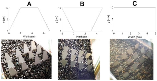
Figure 1.
Sketches and real pictures of vegetation model type (A–C).
As can be seen in Figure 1, the width of the vegetation models varies linearly in the vertical direction for types A and B and it is constant for type C. The general form of linear functions is , where w is the width of the elements, and, a and b are constants that can be easily determined. The linear function of width variation in the vertical direction for type A is and for type B is . The cumulative frontal area of model vegetations can be obtained by integrating the width functions over vegetation height , which is 10 cm:
Vegetation models used in this study are not meant to represent real plant morphology, but the vertical density variation of these models (Figure 2) is similar to natural aquatic plants found in nature (type A is similar to Typha and type C is similar to Rotata) [19].
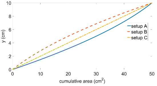
Figure 2.
The cumulative area of vegetation models vs. vegetation height.
Flume experiments were conducted in the hydraulics laboratory of the Water Research Institute of Iran. The flume was 13 m long and 0.45 m wide, and the vegetation patch was located at approximately 8 m. Gravel with d50 of 1.5 cm was used to cover the bed. The velocity of the flow was measured using a propeller velocimeter, which measures the flow velocity only in one direction. Five velocity profiles were measured in each section with eight points measured in the vertical direction in each profile. The measurements were carried out three times for 20 s each, and the mean value was considered as the velocity value. The x, y, and z are the longitudinal, vertical, and lateral directions, respectively. The vegetation patch configuration and location of the velocity profiles are shown in Figure 3.
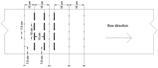
Figure 3.
Plan sketch of vegetation elements and velocity profiles (X marks). The vertical lines (1, 2, 3, and 4) are the cross-sections.
4. Results
The Froude number was approximately 0.4 for all three tests, indicating subcritical flow conditions. The maximum velocity was 1.05 m/s, which occurred for vegetation type B at y = 20 cm; hydraulic parameters of the three tests are reported in Table 1. The velocity, depth, and bed shear stress used in Equations (3) and (8), were averaged cross-sectionally and then between upstream and downstream sections. Having measured depth and the velocity at the upstream and downstream sections, Sf was calculated using Equation (7) and then Cd and n were calculated.

Table 1.
Hydraulic parameters of the three tests.
It should be noted that vegetation density, distribution of patches, submergence ratio, vegetation spacing, bed roughness, and flexibility of the elements are the same for all cases. Therefore, any difference in flow parameters must be caused by the difference in the vertical distribution of density. Vegetation model B produced 25% more drag than model C, which has a uniform distribution of density. Model A led to 12.5% less drag than model C, and model B’s drag coefficient was 41% more than that of model A’s. The results indicate that vertical non-uniformity of vegetation impacts the drag coefficient produced by them.
As mentioned before, eight points were measured in each velocity profile. The measured points were located at y = 3, 4, 5, 7, 10, 15, and 20 cm, and the water surface was different for each case. The velocity could not be measured in the vegetated region (from y = 0 to y = 10 cm of section 2) as it was impractical to do so with a propeller velocimeter. Figure 4a shows the velocity profiles of vegetation model type C (uniform distribution) in the middle of the channel (z = 22.5 cm). At the upstream (section 1), the velocity profile is similar to typical gravel bed velocity profiles but at 15 cm downstream of the vegetation patch (section 3), the velocity profile is altered drastically. The flow is retarded in the vegetated region (from y = 0 to y = 10 cm) and accelerated in the upper region (from y = 10 cm to the water surface), which is the typical velocity profile within submerged vegetation [1,4]. The flow is non-uniform and the depth of the water has decreased from 24 cm to 21 cm. The flow is recovering from vegetation effects in section 4 and it is showing signs of reverting to the profile from section 1.
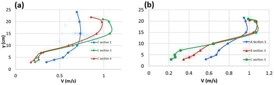
Figure 4.
(a) The velocity profiles of the first, third, and fourth cross-sections of model type C, (b) The velocity profiles of type A, B, and C model vegetation at the third cross-section.
Figure 4b shows the section 3 velocity profiles of model vegetation A, B, and C in the middle of the channel. The velocity profiles are discernably impacted by the vertical distribution of density. Among the velocity profiles of the three vegetation models, model type A has a higher resemblance to the velocity profile upstream of the vegetation patch, meaning that it has suffered less of an impact in comparison to types B and C. Even though the density of model A is higher near the bed, the water has been able to flow easily within the vegetated region since the blockage in the upper part of model A is lower than in models B and C. As for models B and C, the difference in velocity between the vegetated region and the upper region is higher for them because they experience a higher blockage in the vegetated region and the flow, therefore, has been diverted to the upper region, causing a steeper water level gradient and a rapid rise of velocity at the upper region. This effect can also be seen from the velocity contours of the tests on the y-z plane (Figure 5). The velocity has risen rapidly in a short span in the upper region for vegetation type B, but it has risen more gradually for vegetation type A as model B causes more blockage at the top of the vegetation, whereas water has more freedom at the top of vegetation type A. For test A section 1, the velocity has been decreased at the water surface near the walls, indicating the occurrence of the dip phenomena near the walls. The first section of the three tests was nearly identical therefore only the first section of test A is plotted. The velocity contours cover from z = 7.5 cm to z = 37.5 cm in the z direction as the lateral velocity profiles were measured at 7.5 cm from the walls (Figure 3).
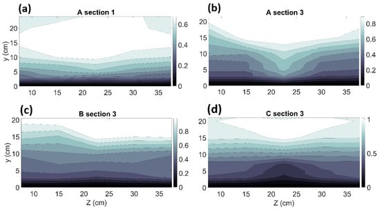
Figure 5.
Velocity contours on the z-y plane for (a) case A section 1, (b) case A section 3, (c) case B section 3, (d) case C section 3.
In order to characterize the distribution of density in the vertical direction, the distance from the bed to the geometric center of model vegetation (yc) has been used as a parameter. The value of this parameter for vegetation model type A, B, and C is 4.33 cm, 5.66 cm, and 5 cm, respectively. As it is apparent from Figure 6, there is a direct relation between yc and both drag and Manning’s coefficient.
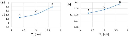
Figure 6.
The relation between yc and the drag coefficient (a), yc and Manning’s coefficient (b).
5. Discussion
As mentioned earlier, the vertical distributions of the vegetation density of model types A, B, and C are similar to some of the aquatic plants found in nature. However, the general shapes of the elements used in this study are different from natural vegetation. Therefore, the absolute values of the drag and Manning’s coefficient are not to be used for modeling vegetated flows with natural plants. In this study, determining parameters of the flow and vegetation, such as density, distribution, spacing, incident velocity, and submergence ratio, were kept constant. Therefore, any distinction in flow structure and flow resistance is attributable to the non-uniform distribution of density in the vertical direction.
Vegetation models with a higher geometric center (yc) have produced higher flow resistance (Figure 6). This finding is in line with other studies. Wu and Cox (2016) reported that vegetation with a lower geometric center led to decreased wave attenuation capability as opposed to vegetation with the same density but with a uniform vertical distribution of density [14]. Jalonen et al. (2013) reported that vegetation with a lower geometric center caused less drag force [18]. It should be noted that these studies do not explicitly address the distance from the bed to the geometric center, and these observations are based on interpretations. Performing a regression analysis for the data in Figure 6, a second-order polynomial function led to the highest coefficient of determination (R2), meaning that the flow resistance is proportional to the second power of the geometric center height ( and ). However, this proportionality may not hold across a broader range of yc or for various flow conditions. Therefore, more data are needed to assess the relation between yc and the flow resistance.
Numerous studies show that plant morphology affects the flow structure and turbulence characteristics [12,19,28,29]. However, these studies mostly focus on the effect of vegetation posture on flow characteristics relevant to plant scale or patch scale such as turbulence, mixing layers, plant chemical uptake, etc. At the reach scale, the flow resistance is the primary subject of study. Nikora et al., (2008) reported that the flow resistance due to vegetation at the reach scale is a function of the blockage factor (the portion of the cross-section occupied by vegetation) and other parameters are not as influential [7]. The results of this study are therefore specifically important because they show that vertical distribution of vegetation density is a relevant parameter of vegetation even for reach scale studies. Moreover, this study addresses the question posed by researchers as to how detailed the morphological characterization of vegetation should be for a specific purpose of study [1,10].
Aquatic plants found in nature are usually flexible to different degrees and the plants bend when subject to high velocities. This effect, which is called reconfiguration of vegetation, leads to a reduction in the frontal area of the plants and consequently a reduction in drag force. The drag force is further reduced because the plants become streamlined [30,31]. The findings of this study show that a lower geometrical center leads to a reduction in the drag force. When aquatic plants bend subject to high velocities, it is inevitable that the plant’s geometrical center will move closer to the bed. This could be a potential cause of drag reduction along with streamlining and reduction of frontal area. To the authors’ knowledge, this effect has not been explicitly outlined in previous research; more exploration is required to investigate this hypothesis.
As can be seen in Figure 4 and Figure 5, different vertical distributions of density led to distinct flow fields. A higher geometrical center (type B) led to higher retardation of the flow at the top of the vegetation but in the case of a lower geometrical center (type A), the flow suffered less impact as less blockage was present at the top of the vegetation. The velocity is naturally lower near the bed and it rises in the vertical direction. Vegetation type A, which has a lower geometrical center is subject to a flow with relatively low velocity and therefore does not produce as much momentum loss as the type B model, which has a higher geometrical center and is subject to a relatively high-velocity flow. Moreover, it has been suggested that when an inflection point in the velocity profiles within vegetation is present, the shear layer at the interface between the vegetated region and the upper region is unstable and Kelvin–Helmholtz vortices are likely to occur [1,32]. These vortices cause vertical momentum exchange and, therefore, lead to a momentum loss in the channel direction [33]. An inflection point has occurred in the velocity profiles for all cases, indicating the presence of these vortices. The velocity contour of model type B shows more blockage in the vegetated region and at the top of the vegetation, and an abrupt rise of velocity in the upper region, which could be attributable to more intense shear instabilities at the top of the vegetation in comparison to model types A and C. Alteration of the velocity profiles and the flow field caused by vertical distribution of density has implications for bed shear stress and consequently morphological processes. The value of cross-sectionally averaged bed shear stress for the first section of the tests is 6.8 N/m2 and for the third section of the tests, the values for A, B, and C types are 13.5, 17, and 19.8 N/m2, respectively. A steeper water surface gradient and increased velocities for model types B and C have caused the bed shear stress to increase.
6. Conclusions
In order to study the effect of vertical variation of submerged vegetation density on the flow resistance and bulk flow characteristics, three patches of wooden model vegetation elements were compared. The vegetation models had the same density but different vertical distributions of density. All other effective parameters were kept constant so that any difference in the flow structure and the flow resistance would be attributable to the distribution of density in the vertical direction.
A force balance approach was employed to calculate the drag coefficient. The three vegetation models led to different values of drag and Manning’s coefficient. There was as much as a 41% difference in the value of the drag coefficient produced by the models. The distance from the bed to the geometrical center of vegetation was used as a parameter to characterize the vertical variation of density. There was a direct relation between this parameter with both the drag coefficient and Manning’s coefficient, showing a second power relation to the height of the geometrical center. More data are needed to assess the obtained proportionality as it may not hold across a wider range the flow conditions and vegetation characteristics. The vertical distribution of vegetation density is a key influential vegetation parameter even in reach scale studies as it affects the flow resistance substantially.
The flow fields of the three vegetation models present distinct characteristics, showing different behaviors in the vegetated region, the upper region, and the interface between these regions. The vegetation model with a higher geometrical center leads to intensified loss of momentum in the vegetated region and at the top of the vegetation. Vegetation with a lower geometrical center causes the least impact on the flow as the majority of its area is close to the bed and it is subject to a relatively low velocity. The vertical variation of vegetation density affects the bed shear stress as well.
With the advancements made in Lidar techniques and remote sensing in general, it is now easier to capture detailed vegetation morphology. The findings of this study can help researchers and practitioners use relevant vegetation parameters in resistance prediction.
Author Contributions
Conceptualization, S.D. and H.A.; methodology, H.A.; software, E.D. and H.R.; resources, H.A.; writing—original draft preparation, S.D., E.D., H.R.; writing—review and editing, S.D., E.D., H.A., M.N.-S., H.R.; supervision, H.A., M.N.-S., M.K.; All authors have read and agreed to the published version of the manuscript.
Funding
This research received no external funding.
Institutional Review Board Statement
Not applicable.
Informed Consent Statement
Not applicable.
Data Availability Statement
The data are available upon request.
Conflicts of Interest
The authors declare no conflict of interest.
References
- Nepf, H.M. Hydrodynamics of vegetated channels. J. Hydraul. Res. 2012, 50, 262–279. [Google Scholar] [CrossRef]
- Osterkamp, W.R.; Hupp, C.R.; Stoffel, M. The interactions between vegetation and erosion: New directions for research at the interface of ecology and geomorphology. Earth Surf. Process. Landf. 2012, 37, 23–36. [Google Scholar] [CrossRef]
- Marois, D.E.; Mitsch, W.J. Coastal protection from tsunamis and cyclones provided by mangrove wetlands—A review. Int. J. Biodivers. Sci. Ecosyst. Serv. Manag. 2015, 11, 71–83. [Google Scholar] [CrossRef]
- Wang, C.; Zheng, S.S.; Wang, P.F.; Hou, J. Interactions between vegetation, water flow and sediment transport: A review. J. Hydrodyn. 2015, 27, 24–37. [Google Scholar] [CrossRef]
- Tempest, J.A.; Möller, I.; Spencer, T. A review of plant-flow interactions on salt marshes: The importance of vegetation structure and plant mechanical characteristics. Wiley Interdiscip. Rev. Water 2015, 2, 669–681. [Google Scholar] [CrossRef]
- Tinoco, R.O.; San Juan, J.E.; Mullarney, J.C. Simplification bias: Lessons from laboratory and field experiments on flow through aquatic vegetation. Earth Surf. Process. Landf. 2020, 45, 121–143. [Google Scholar] [CrossRef]
- Nikora, V.; Larned, S.; Nikora, N.; Debnath, K.; Cooper, G.; Reid, M. Hydraulic resistance due to aquatic vegetation in small streams: Field study. J. Hydraul. Eng. 2008, 134, 1326–1332. [Google Scholar] [CrossRef]
- D’Ippolito, A.; Calomino, F.; Alfonsi, G.; Lauria, A. Flow resistance in open channel due to vegetation at reach scale: A review. Water 2021, 13, 116. [Google Scholar] [CrossRef]
- Derakhshan, S.; Afzalimehr, H.; Singh, V.P. Effect of vegetation patch distribution on the flow resistance. Int. J. Hydraul. Eng. 2021, 10, 19–25. [Google Scholar]
- Shields, F.D.; Coulton, K.G.; Nepf, H. Representation of vegetation in two-dimensional hydrodynamic models. J. Hydraul. Eng. 2017, 143, 02517002. [Google Scholar] [CrossRef]
- Ozeren, Y.; Wren, D.G.; Wu, W. Experimental investigation of wave attenuation through model and live vegetation. J. Waterw. Port Coast. Ocean. Eng. 2014, 140, 04014019. [Google Scholar] [CrossRef]
- Boothroyd, R.J.; Hardy, R.J.; Warburton, J.; Marjoribanks, T.I. The importance of accurately representing submerged vegetation morphology in the numerical prediction of complex river flow. Earth Surf. Process. Landf. 2016, 41, 567–576. [Google Scholar] [CrossRef]
- Huai, W.X.; Zhang, J.; Katul, G.G.; Cheng, Y.G.; Tang, X.; Wang, W.J. The structure of turbulent flow through submerged flexible vegetation. J. Hydrodyn. 2019, 31, 274–292. [Google Scholar] [CrossRef]
- Wu, W.C.; Cox, D.T. Effects of vertical variation in vegetation density on wave attenuation. J. Waterw. Port Coast. Ocean. Eng. 2016, 142, 04015020. [Google Scholar] [CrossRef]
- He, F.; Chen, J.; Jiang, C. Surface wave attenuation by vegetation with the stem, root and canopy. Coast. Eng. 2019, 152, 103509. [Google Scholar] [CrossRef]
- Wu, W.C.; Ma, G.; Cox, D.T. Modeling wave attenuation induced by the vertical density variations of vegetation. Coast. Eng. 2016, 112, 17–27. [Google Scholar] [CrossRef]
- Lou, S.; Chen, M.; Ma, G.; Liu, S.; Zhong, G. Laboratory study of the effect of vertically varying vegetation density on waves, currents and wave-current interactions. Appl. Ocean. Res. 2018, 79, 74–87. [Google Scholar] [CrossRef]
- Jalonen, J.; Järvelä, J.; Aberle, J. Leaf area index as vegetation density measure for hydraulic analyses. J. Hydraul. Eng. 2013, 139, 461–469. [Google Scholar] [CrossRef]
- Xu, Y.; Nepf, H. Measured and predicted turbulent kinetic energy in flow through emergent vegetation with real plant morphology. Water Resour. Res. 2020, 56, e2020WR027892. [Google Scholar] [CrossRef]
- Zhao, M.D.; Fan, Z.L. Emergent vegetation flow with varying vertical porosity. J. Hydrodyn. 2019, 31, 1043–1051. [Google Scholar] [CrossRef]
- Klemas, V.V. Remote sensing of submerged aquatic vegetation. In Seafloor Mapping along Continental Shelves; Springer: Berlin/Heidelberg, Germany, 2016; pp. 125–140. [Google Scholar]
- Abu-Aly, T.R.; Pasternack, G.B.; Wyrick, J.R.; Barker, R.; Massa, D.; Johnson, T. Effects of LiDAR-derived, spatially distributed vegetation roughness on two-dimensional hydraulics in a gravel-cobble river at flows of 0.2 to 20 times bankfull. Geomorphology 2014, 206, 468–482. [Google Scholar] [CrossRef]
- Rowan, G.S.; Kalacska, M.J.R.S. A review of remote sensing of submerged aquatic vegetation for non-specialists. Remote Sens. 2021, 13, 623. [Google Scholar] [CrossRef]
- Shucksmith, J.D.; Boxall, J.B.; Guymer, I. Bulk flow resistance in vegetated channels: Analysis of momentum balance approaches based on data obtained in aging live vegetation. J. Hydraul. Eng. 2011, 137, 1624–1635. [Google Scholar] [CrossRef]
- Tang, H.; Tian, Z.; Yan, J.; Yuan, S. Determining drag coefficients and their application in modelling of turbulent flow with submerged vegetation. Adv. Water Resour. 2014, 69, 134–145. [Google Scholar] [CrossRef]
- Liu, X.; Zeng, Y. Drag coefficient for rigid vegetation in subcritical open-channel flow. Environ. Fluid Mech. 2017, 17, 1035–1050. [Google Scholar] [CrossRef]
- Zhang, Y.; Wang, P.; Cheng, J.; Wang, W.J.; Zeng, L.; Wang, B. Drag coefficient of emergent flexible vegetation in steady nonuniform flow. Water Resour. Res. 2020, 56, e2020WR027613. [Google Scholar] [CrossRef]
- Afzalimehr, H.; Anctil, F. Accelerating shear velocity in gravel-bed channels. Hydrol. Sci. J. 2000, 45, 113–124. [Google Scholar] [CrossRef]
- Boothroyd, R.J.; Hardy, R.J.; Warburton, J.; Marjoribanks, T.I. Modeling complex flow structures and drag around a submerged plant of varied posture. Water Resour. Res. 2017, 53, 2877–2901. [Google Scholar] [CrossRef]
- Luhar, M.; Nepf, H.M. Flow-induced reconfiguration of buoyant and flexible aquatic vegetation. Limnol. Oceanogr. 2011, 56, 2003–2017. [Google Scholar] [CrossRef]
- Verschoren, V.; Meire, D.; Schoelynck, J.; Buis, K.; Bal, K.D.; Troch, P.; Meire, P.; Temmerman, S. Resistance and reconfiguration of natural flexible submerged vegetation in hydrodynamic river modelling. Environ. Fluid Mech. 2016, 16, 245–265. [Google Scholar] [CrossRef]
- Nepf, H.; Ghisalberti, M. Flow and transport in channels with submerged vegetation. Acta Geophys. 2008, 56, 753–777. [Google Scholar] [CrossRef]
- Ghisalberti, M.; Nepf, H.M. Mixing layers and coherent structures in vegetated aquatic flows. J. Geophys. Res. Ocean. 2002, 107, 3-1–3-11. [Google Scholar] [CrossRef]
Publisher’s Note: MDPI stays neutral with regard to jurisdictional claims in published maps and institutional affiliations. |
© 2022 by the authors. Licensee MDPI, Basel, Switzerland. This article is an open access article distributed under the terms and conditions of the Creative Commons Attribution (CC BY) license (https://creativecommons.org/licenses/by/4.0/).