Article

Influence of Land Use Changes on the Longaví Catchment Hydrology in South-Center Chile

1
Department of Civil Engineering, University of Siegen, 57076 Siegen, Germany
2
Escuela de Agronomía, Pontificia Universidad Católica de Valparaíso, Quillota 2260000, Chile
3
Centro Regional de Investigación e Innovación para la Sostenibilidad de la Agricultura y los Territorios Rurales (CERES), Quillota 2260000, Chile
*
Author to whom correspondence should be addressed.
Hydrology 2022, 9(10), 169; https://doi.org/10.3390/hydrology9100169
Submission received: 25 August 2022 / Revised: 20 September 2022 / Accepted: 25 September 2022 / Published: 28 September 2022

Abstract

:
During recent decades, the South-Central part of Chile has shown strong vulnerability due to the effects of land use change (LUC). The interaction of these changes with local hydrology has not been adequately investigated and is poorly understood, especially in mountainous areas under irrigated agriculture. We applied the SWAT + agrohydrological model to study the effects of LUC on hydrological fluxes in the Longaví catchment, Maule region, South-Central Chile. Land use maps (LUMs) from 1997, 2009, and 2016 were used in conjunction with a 41-year (1979–2019) hydro-meteorological series of daily observations as forcing data. The dominant changes in land use during the study period relate to agriculture, shrublands, forestry of exotic species, and urban sprawl. First, the LUM of 1997 was used for model setup, sensitivity analysis, calibration, and validation. Second, the impact of LUC documented through LUMs 2009 and 2016 was analyzed. Our analysis clearly reveals that the overall water balance and internal moisture redistribution in the Longaví catchment have been considerably affected by decreases in precipitation, changes in land use and water use practices. Unless a comprehensive regulatory system is introduced that addresses current climatic conditions and territorial use, it is likely that the decrease in water resources will persist and worsen through climate changes.

1. Introduction

Human-induced processes and natural system changes can cause alterations in the landscape with corresponding environmental impacts on both natural and human systems [1,2]. In particular, land use changes (LUC) attributable to human activities can have potential impacts on catchment hydrology [3], and as a result on water resources availability [4]. At basin scale, particular land management practices and alterations in the use of the territory can affect the partitioning and redistribution of water between various flow pathways and system components [5]. Affected processes include precipitation interception by the canopy, where the type of vegetation can influence the interception rate (i.e., native or exotic species) [6,7]. In addition to evapotranspiration, infiltration, runoff generation, and surface flow pattern [8], as well as soil erosion [9].
In Chile, a country that is known for its important mining sector, agricultural crop production, and forestry [10], anthropogenic changes in land use are a very common practice and are justified at the institutional level by the need to support the socio-economic development of specific regions [11]. These types of land use changes are intertwined with the local climate, the productive capacity of particular areas, soil conditions, and the possibility of fostering exotic tree plantations (i.e., Pinus radiata and Eucalyptus globulus) [10]. In addition, some policy management allowed the transition from natural forest cover to other types of land use, including exotic tree plantations, intensive irrigated agriculture, and urban development, particularly from 1994 to 2014 [12,13,14]. For instance, 67% of Chilean temperate forests were lost by deforestation between 1975 and 2000 [15]. As a result, a large part of the country has undergone rapid land use change, with large areas that were originally covered by native vegetation becoming the subject of commercial plantation forestry [12,16] and intensive agriculture exploitation [11,15].
To satisfy agricultural demand, the irrigation water use is estimated to be around 77% to 85% of the total available freshwater in the country [17,18]. However, the overall lack of monitoring, among others due to scarcity of observing stations, hampers the quantification and estimation of available water, including surface flow and groundwater extractions [17,19]. In addition, an annual rainfall deficit from 25 to 45% has been reported since 2010, increasing water scarcity in the center of the country [18]. As consequence, the lack of an efficient water use governance leads to conflicts related to water overuse [20,21], resulting in unequal redistribution among water users affecting the basin hydrology.
To understand and evaluate the impacts of LUC on runoff and water availability, hydrological models constitute important and widely used investigation tools [22,23]. Particularly physical-based hydrological models allow one to describe the complex interaction between LUC and various components of the hydrological cycle in detail [24,25]. Continuous-time models, such as the Soil and Water Assessment Tool + (SWAT+) based on the original version of SWAT [26,27], support the evaluation and quantification of the impacts of different land management practices on water resources with varying soils and land use over long periods of time [28]. Thanks to the possibility to assess specific land management practices in agricultural systems and forest production, among many other processes, SWAT has been widely applied in different watersheds around the world [29,30,31].
The application of SWAT in Chile is not new. Some studies have been carried out using SWAT as a hydrological model with the aim of assessing the impacts of land use changes in Chile. These applications remain limited to mountain areas in proximity to the coast [32,33,34,35] or to the analysis of the impacts of climate change on snow accumulation [36,37]. Thus, the applicability of SWAT+ related to land use change in the rugged terrain of South-Central Chile has not yet been investigated, particularly in data-poor regions and/or irrigated agricultural areas.
Our chosen study area, the Longaví catchment, is a sub-entity of the Loncomilla river, located in the mountainous area of South-Central Chile. The main human activities in the area are related to agriculture and exotic tree plantations, established especially during the last few decades. Unfortunately, the impact of such land use management practices is not well understood, particularly with regard to the effects on specific hydrological processes, soil erosion, and overall basin water balance. Although it has become evident that the flow rate of rivers and precipitation has decreased, there is no information on the impacts of both precipitation and land use change effects on the catchment hydrology. The aim of this study is, therefore, a process-based analysis to evaluate how the combined effect of changes in precipitation and land use changes in the Longaví catchment has affected hydrology over a total period of 30 years. Given the similarity of territory and land management practices, our results can be extrapolated to similar systems in the region.

2. Materials and Methods

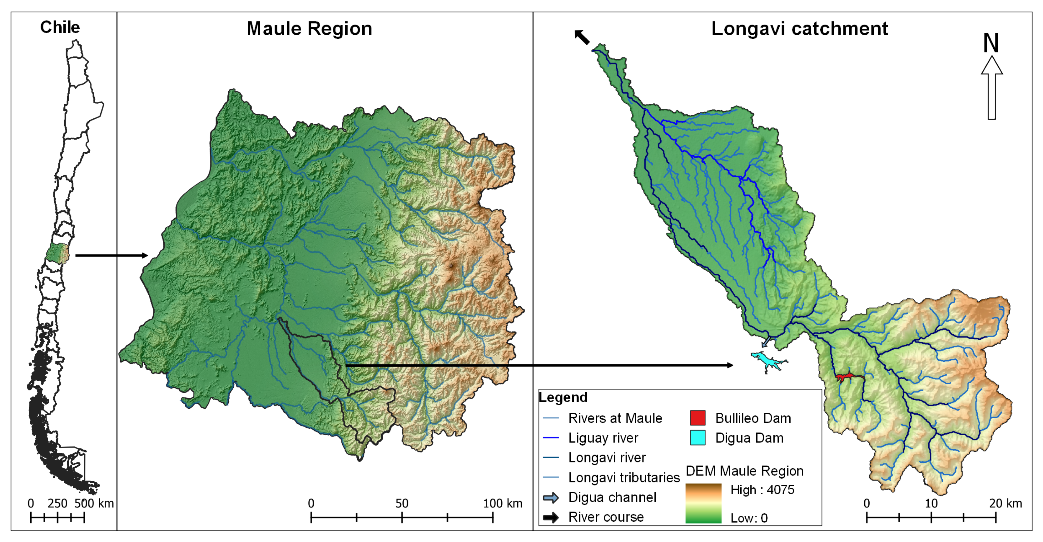
The Longaví catchment is located in the Maule region, VII Region of Chile, between latitude 35°49′ S and longitude 71°47′ W. The watershed encompasses an area of 1387 km2 (Figure 1). The geology of the basin is characterized by the presence of intrusive rocks, sedimentary, volcano, and volcano-sedimentary sequences [38], and elevations ranging from 102 m to 3174 m above sea level. The river basin is dominated by temperate-Mediterranean climate and annual total precipitations of around 1669 mm year−1, with a dry summer of 74 mm year−1 (January, February, March), a rainy autumn of 746 mm year−1 (April, May, June) and winter of 682 mm year−1 (July, August, September), with regular snow accumulation in the mountain areas, and a variable spring of 746 mm year−1 (October, November, December) [39]. Concerning temperatures, maximum mean values of 24.6 °C for the summer season and minimum mean values of 0.5 °C for the winter season have been recorded in the study area over 41 years of continuous hydro-meteorological observation (temperatures and precipitation) [39].
With reference to existing local water management infrastructure, the Bullileo Dam operated by “Junta de Vigilancia del Río Longaví y sus Afluentes” (Longaví river surveillance board) stores water for irrigation mainly during drought periods. In addition, the Digua channel transfers water from the Longaví river to the Digua Dam, which is situated outside the watershed boundaries.

2.1. Swat+ Model Description

The Soil and Water Assessment Tool + (SWAT+) is a semi-distributed hydrological model that has been especially developed for agro-hydrological impact studies on management practices and climate-water interactions, as well as the transport of nutrients and pesticides on a basin scale [28]. SWAT + reproduces most of the physical processes of the hydrological cycle in different time steps on the basis of multiple data inputs, such as hydro-meteorological forcing, topography, soil parameters, land use, and land management information, including crop rotation [28,40]. With this input information, the hydrologic cycle can be simulated based on the basis of 1-dimensional water mass balance and steady-state momentum conservation across adjacent vertical soil columns (Equation (1)) [26,31]. The water balance equation for a soil column cell is stated as follows [26]:
S W t = S W o + i = 1 t ( P r S u r q L a t q E T P e r c )
where S W t is the soil water content (mm) in time step t, S W o is the initial soil water content (mm), P r is the amount of precipitation on day i (mm), S u r q is the amount of surface runoff on day i (mm) and is estimated using the Soil Conservation Service (SCS) curve number equation, L a t q is the amount of lateral subsurface flow to the channel on day i (mm), and it is originated from the saturated zone of soil layers and contributes to the stream flow calculated in each layer by a kinematic storage model, E T is the amount of actual evapotranspiration on day i (mm), P e r c is the amount of percolation of soil water from the bottom of the soil profile on day i (mm), and is calculated as the sum of three terms: F l o (Return Flow), R c h r g (Recharge to deep aquifer) and R e v a p (Plant water uptake and evaporation). Additionally, the sum of S u r q and L a t q can be expressed as W Y (Water yield).

2.2. Model Setup

In this study, SWAT+ (v. 2.0.4) was interfaced with QSWAT+ (v. 2.0.6), an open-source graphical user interface [41], and the sub-basin scheme derived from the digital elevation model (DEM). To represent the river and natural flow paths, a topographic analysis is performed, leading to a drainage direction map with respective downhill cell interconnectivity. The headwaters streams and the river network were defined considering the point of union with the Loncomilla River and a threshold area (Figure 1). The final network extent was verified against the network observable from remotely sensed images. To complete the model, Bullileo Dam was added as a storage entity to the network structure with its specific area and volume information.
Hydrological Response Units (HRUs) as basic spatial modeling entities were generated on the basis of raster images and topographic analysis by merging slope maps from the DEM, soil type, and land use maps. Meteorological forcing data at the daily time step for the hydrological processes have been pre-processed and readied for model use. For the calculation of the potential evapotranspiration (PET), the elaborate Penman-Monteith formulation was used.

2.2.1. Topography, Soil, Hydro-Meteorological, and Discharge Data

The input parameters are presented in Table 1. The DEM was obtained from the Shuttle Radar Topography Mission (STRM) dataset with 90 × 90 m spatial resolution [42].
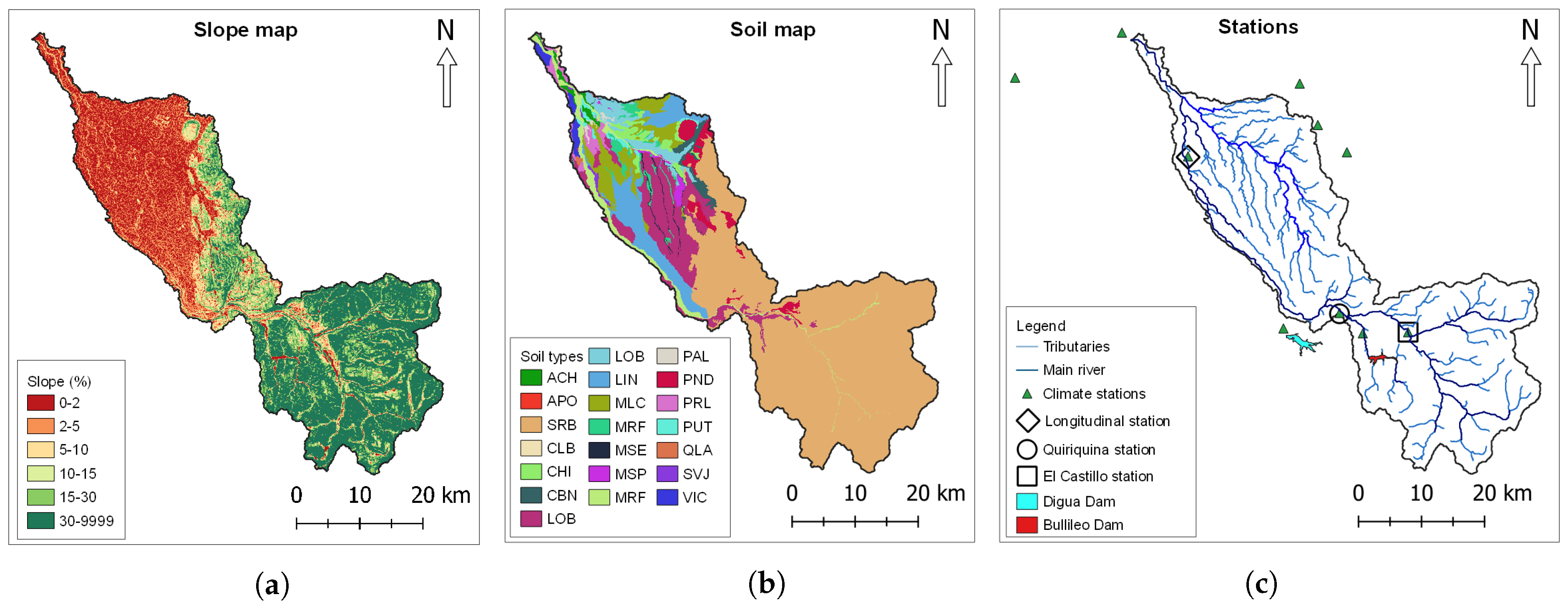
The slopes of the land surface were subdivided into six categories (Figure 2a) based on topographic information extracted from the DEM. The data on soil properties required for completion of the input database of the model were acquired during a field campaign in the catchment. The field data set was complemented with soil properties data from agricultural science studies of the VIIth administrative region that were conducted by the Natural Resources Information Center (CIREN) in 1997. In summary, a comprehensive soil type map for the study area was generated, which includes the 21 soil types described by CIREN [43] (Figure 2b).
In addition, soil samples under different land use types were taken in the field to corroborate and complement the soil physicochemical information provided by CIREN (Table 2). Soil data like bulk density (BD), soil carbon content (CBN), saturated hydraulic conductivity (K), pH, and soil texture were determined through fieldwork in the framework of this study. The analysis of the soil samples was carried out using the Laboratory of Soils and Foliar Analysis of Pontificia Universidad Católica de Valparaíso (PUCV). According to CIREN [43], the predominant soil textures in the catchment are loamy sand soils (71.5%) developed from basic volcanic materials, loamy silt soils (10.5%) originated from volcanic ashes and sedimentary deposits, and loam soils (10.2%) with an alluvial origin and sediment deposits.
The hydro-meteorological input data for the years 1979 to 2019 were acquired from the Catchment Attributes and Meteorology for Large-sample Studies-Chile dataset (CAMELS-CL), taking as a reference 10 climate stations for precipitation and temperatures (daily minimum and maximum) located in the surrounding area of the study area (Figure 2c, Table 1). Due to scarcity of in-situ data in Longaví, time series of wind velocity and relative air humidity from the nearby stations of the mountain area of Mataquito river basin, Maule region, were used. These data were supplied by “Dirección General de Agua” (DGA), the Central Water Directorate. Solar radiation data were obtained from “Explorador Solar” of the Chilean Ministry of Energy [45].
Three discharge stations are operated in the Longaví river network. Rio Longaví en Longitudinal (Longitudinal), located between 36°00′ S latitude and 71°43′ W longitude, has only a very short data record with few months of discharge measurements covering the period 1979 to 1985. Because of the limited usability of those records, two additional discharge stations were used instead with longer records: Quiriquina station, located between 36°23′ S latitude and 71°46′ W longitude, and El Castillo station, located between 36°15′ S latitude and 71°20′ W longitude [39]. Both the Quiriquina and El Castillo stations have discharge data available that cover the 1979 to 2019 period. Nevertheless, the time series are partially incomplete, with some gaps and unreliable discharge peak values.

2.2.2. Land Use Maps and Land Use Management in SWAT+

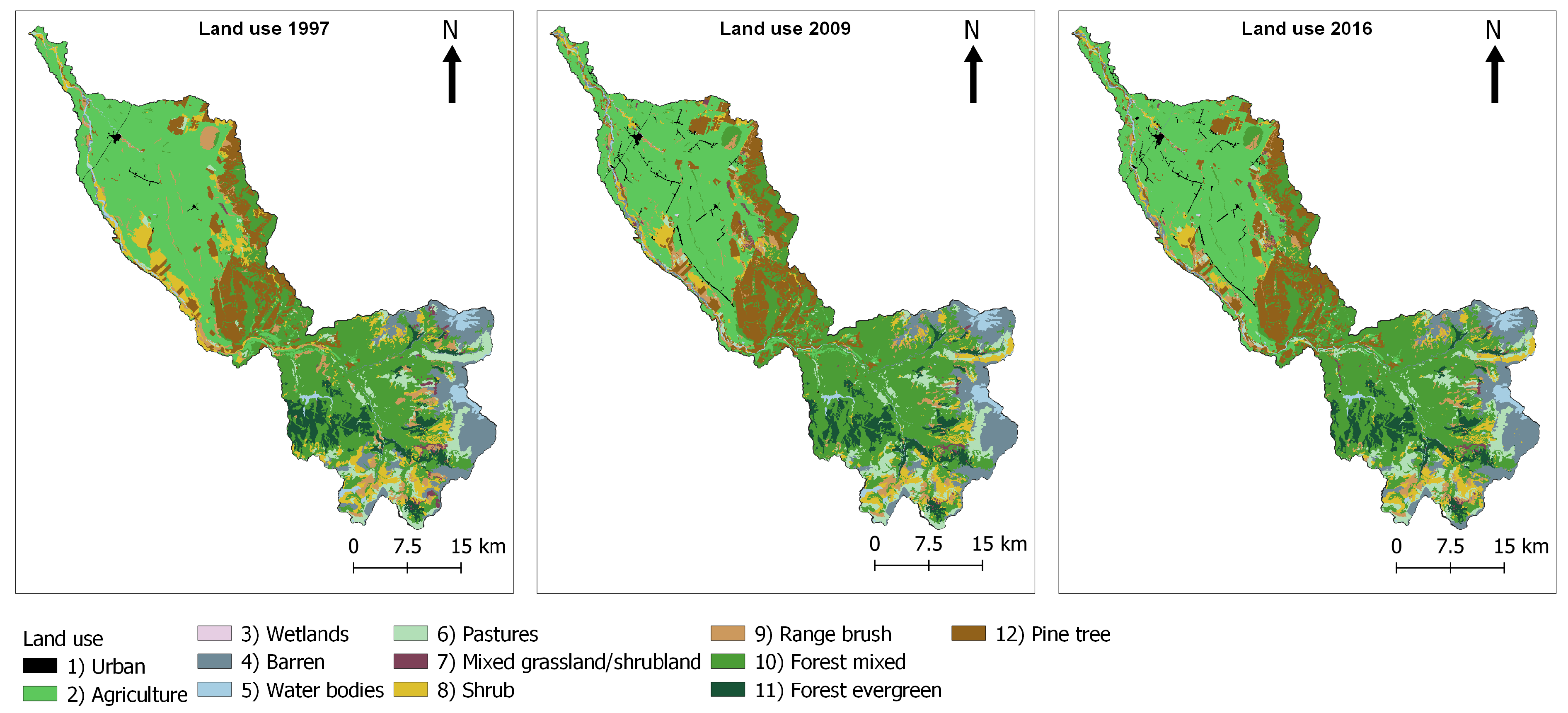
The land use (LU) maps of 1997, 2009, and 2016 were obtained from the National Forest Corporation (CONAF) [44], following the LU classifications into 12 categories (Figure 3).
The main land use types in the basin (Table 3) were agriculture with 416.8 km2 (LU 1997), in addition to mixed deciduous and evergreen forests that covered an area of 414.7 km2 (LU 2009) and 415.5 km2 (LU 2016). For the studied periods, the most dominant land use types were agriculture (>28%), followed by forest mixed (>27%) and pine tree plantations (>9%). Between the years 1997 and 2016, the most important increase took place with mixed forests and pine tree plantations, with values that range between 2.67% (37.0 km2) and 1.70% (23.7 km2) respectively, followed by urban developments with 0.55% (7.6 km2) of incremental extension. The highest areal reduction was recorded for shrublands with −2.50% (−34.7 km2) and agriculture with a reduction of −1.42% (−19.7 km2), followed by evergreen forests with −0.23% (−3.2 km2).
The management schedules for agriculture, forest mixed and pine tree plantations were implemented in the model as pre-defined operations using conditions and actions inserted into the SWAT+ decision tables system [40]. Following the decision tables logic for automatic management schedules, the conditions of “plant” and “harvest” every 20 years were implemented for forest mixed. In the case of pine tree plantations, an automatic management schedule with “plant” and “harvest and kill” every 20 years were assigned in dependence on the pine tree maturity level. For agriculture, an automatic management schedule with “plant”, “harvest and kill”, “rotation and reset” for every year was established, taking as a reference local information from the traditional crops in the studied area. In addition, an auto-application of the furrow irrigation system was assigned under soil-water stress and plant maturity status, whereby the channel is used as a source to satisfy irrigation water demand.

2.2.3. Model Sensitivity Analysis, Calibration and Validation

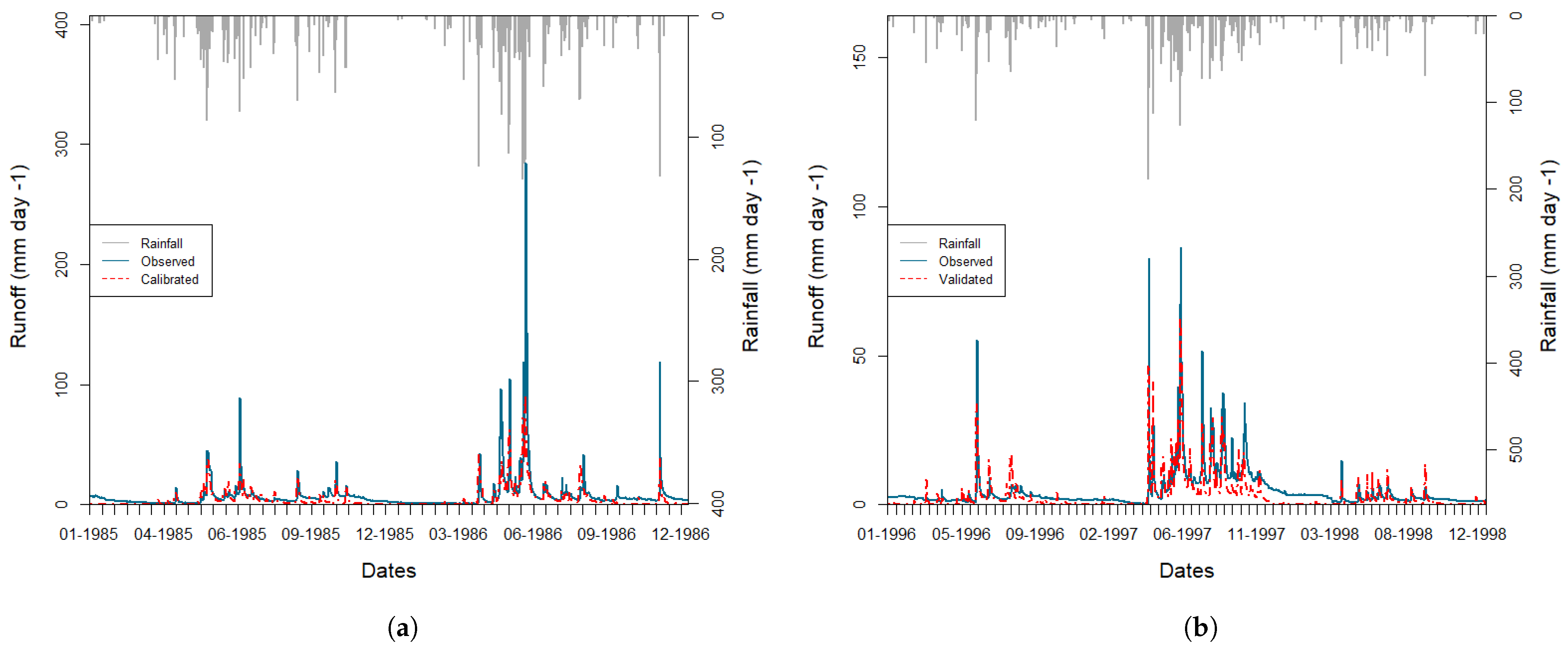
A 41-year period (1979 to 2019) was selected in accordance with available forcing records for simulating runoff processes on a daily time step basis in Longaví, reserving one full year for model warm-up under the land use conditions of 1997. El Castillo and Quiriquina discharge stations were selected for model sensitivity analysis and multi-site model calibration from 1985 to 1986. In addition, El Castillo and Quiriquina stations were used jointly for validation purposes from 1996 to 1998 period, considering the availability and continuity of the data during the study period. A longitudinal station was used to evaluate the baseline simulation output in the lower part of the catchment, mainly to verify the flow after satisfying irrigation demand further upstream.
Global sensitivity analysis and calibration procedures were performed using the tool SWAT+ Toolbox v0.7.6, a sensitivity and automatic calibration module developed with basis on the existing calibration tool IPEAT+ [46]. Following indications from the literature [46,47], a total group of 16 hydrological parameters was selected with the goal of identifying the most sensitive ones for the studied system (Table 4).
After identifying the most sensitive parameters, SWAT+ Toolbox was set up and run with 1000 iterations for the calibration period (1985–1986). After successful calibration, the model was validated over a three-year period (1996–1998) by benchmarking the output against observations recorded at El Castillo and Quiriquina stations in the upper and middle part of the catchment. In this context, usual efficiency criteria were adopted as model performance metrics. For additional verification, cumulative mass analysis on different hydrological fluxes was used. To validate model performance for the entire catchment upstream of the Longaví basin outlet, a Longitudinal station was used to evaluate the irrigation system under the reference scenario. The calibration of the irrigation system was tested under different operating conditions referring to the longitudinal station discharges as a benchmark record. Afterward, a manual calibration of the irrigation system was performed by considering the water demand of the plants under different irrigation schedules.
To examine the effects of past land use changes on the catchment hydrology, the model was set up with land use maps LU 2009 and LU 2016 without any further modification under the same period of hydro-meteorological data (1979–2019). The output consistency of the model was verified for the periods of 2006 to 2009 and 2012 at El Castillo and Quiriquina stations using the different LU maps, respectively. Moreover, changes in components of the catchment hydrology were evaluated on a decadal basis for each LU map (1990–1999, 2000–2009, 2010–2019). The water balance was analyzed by examining the hydrological model components S u r q , L a t q , W Y , R c h r g , and actual E T .

2.3. Efficiency Criteria for Model Evaluation

For model performance verification, the simulated and observed time series from El Castillo and Quiriquina stations were used. Hydrographs were compared first visually, and in a second step, quantitatively using statistical indices such as the coefficient of determination (R2) and goodness of fit measures such as the Nash–Sutcliffe efficiency (NSE), relative Nash–Sutcliffe efficiency (rNSE), the standard deviation ratio of RMSE observations (RSR), and the percent of the model BIAS (PBIAS).
R2 is used to measure the consistency of the simulated model output against the observed data (Equation (2)). The values of R2 vary between 0 and 1, less error variance is indicated by higher values [48,49]:
R 2 = i = 1 n ( Q i o b s Q ¯ o b s ) ( Q i s i m Q ¯ o b s ) i = 1 n ( Q i o b s Q ¯ o b s ) 2 i = 1 n ( Q i s i m Q ¯ s i m ) 2
where Q i o b s and Q i s i m represent the observed and simulated flow during each day. Whereas Q ¯ o b s and Q ¯ s i m are the observed and simulated means, respectively.
NSE is a standardized statistical method that determines the relative magnitude of the residual variance compared to the measured data variance (Equation (3)). NSE values vary from −∞ to 1, where 1 corresponds to a perfect match between the observed and simulated values, and NSE ≤ 0.5 indicate unsatisfactory model performance [49,50]:
NSE = 1 i = 1 n ( Q i o b s Q i s i m ) 2 i = 1 n ( Q i o b s Q ¯ o b s ) 2
The rNSE is a modification of the NSE (Equation (4)), which calculates the efficiency between the simulated and observed data without gaps in the time series [51]:
rNSE = 1 i = 1 n Q i o b s Q i s i m Q i o b s 2 i = 1 n Q i o b s Q ¯ o b s Q ¯ o b s 2
RSR is calculated as the ratio of Root Mean Square Error (RMSE) and standard deviation of the measured data (Equation (5)). An RSR of zero indicates the optimal value, while RSR > 0.7 represents unsatisfactory model performance [50].
RSR = RMSE S T D E V o b s = i = 1 n ( Q i o b s Q i s i m ) 2 i = 1 n ( Q i o b s Q ¯ o b s ) 2
PBIAS measures the estimation bias of the model (Equation (6)). PBIAS values can be positive or negative, indicating underestimation and overestimation, respectively, while the zero values represent the best simulation performance of the model [50].
PBIAS = i = 1 n ( Q i o b s Q i s i m ) * 100 i = 1 n ( Q i o b s )
In order to analyze the calibration and validation periods, recommended ranges of values for each efficiency criterion at daily time step were used [48,49,50].

3. Results

3.1. Sensitivity Analysis

A simulation of 41 years period (1979 to 2019) was made using SWAT+ based on the land use map of 1997, considering in total 40 sub-basins, 255 channels, and 6119 HRUs. Even with field values, the K parameter turned out to be highly sensitive during the sensitivity analysis, possibly due to soil heterogeneity and the regionalization of soil parameters in the model. Therefore, to achieve a better performance of the model, seven parameters were calibrated using a multi-site calibration method considering a minimum and maximum range of sensitive values (Table 5).

3.2. SWAT+ Model Calibration and Validation

Satisfactory model performance, given poor data availability, was achieved for the multi-site calibration method with an NSE value of 0.52. Similarly, acceptable model performance was achieved for both the El Castillo and Quiriquina stations for calibration and validation periods (Table 6).
R2 values are considered good and satisfactory, respectively, albeit they change only marginally from 0.63 in the simulation to 0.64 for the calibration period at the El Castillo station and from 0.58 to 0.57 at the Quiriquina station. According to the classifications of Moriasi et al. [50], during the calibration period, the model showed a satisfactory performance with NSE of 0.53 at El Castillo station (Figure 4a) and 0.50 at the Quiriquina station. In addition, values of rNSE were considerably improved from 0.81 to 0.87 for El Castillo and from 0.75 to 0.83 for Quiriquina station, in both cases rNSE values can be classified as very good. In the case of RSR, with a value of 0.69 for El Castillo and 0.70 for Quiriquina, it can be considered also satisfactory. In the case of PBIAS, the resulting values have been considered unsatisfactory. However, the poor performance can be explained by bias in some unreliable peaks of daily discharge values.
According to the classifications of Moriasi et al. [50], for the validation period, the model showed a satisfactory performance with an NSE of 0.64 for both El Castillo and Quiriquina stations (Figure 4b). In the case of rNSE, values of 0.70 and 0.61 are considered good for the El Castillo station and satisfactory for the Quiriquina station. In the case of RSR, values of 0.58 and 0.59 were considered good for both El Castillo and Quiriquina stations, respectively. Similarly to the calibration period, PBIAS were considered unsatisfactory for both stations, mainly associated with the bias of unreliable discharge peaks.

3.3. Model Performance under Land Use Change

For the evaluation of land use changes, each land use map was replaced in the original model without any further modification. This intervention modified the total number of HRUs created with LU 1997. Starting from 6119 originally, for LU 2009 and LU 2016, the number increased to 6638 and 6708 HRUs, respectively. El Castillo and Quiriquina stations were used to validate the performance of the model with both new land use maps, taking observations for each corresponding decade (Table 7) as a reference base case. To evaluate the model stability, even with scarcity of data, the efficiency criteria were calculated for LU 2009 and LU 2016 for validation periods of 2006–2009 and 2012, respectively, and adopting recommended ranges of values [48,49,50].
For LU 2009 and LU 2016, good and satisfactory model performance were achieved at El Castillo station with R2 0.76 and 0.61, respectively. In addition, good and satisfactory NSE values of 0.66 and 0.56 were obtained. Similarly, rNSE values of 0.78 and 0.83 are considered very good model performance for the El Castillo station. Furthermore, good and satisfactory model performance with values of 0.59 and 0.66 for RSR were estimated, respectively. In the case of the Quiriquina station, for LU 2009 and LU 2016, R2 values of 0.72 and 0.60 were achieved for the LU 2009 and LU 2016, respectively. In addition, a satisfactory NSE value of 0.64 for LU 2009, and good for LU 2016 with NSE of 0.57. For rNSE, good and satisfactory model performance with values of 0.66 and 0.61 were obtained. In the case of RSR, good and satisfactory model performance were estimated with values of 0.60 and 0.66, respectively. Similarly to the calibration period, for PBIAS were considered as unsatisfactory for both stations, mainly associated with the bias of unreliable discharge peaks.

3.4. Past Land Use Change Impacts on the Catchment Hydrology

The results based on each land use map were separated by each respective decade (1990–1999, 2000–2009, 2010–2019). The impacts of past land use changes on the catchment hydrology are presented on a monthly, seasonal, and yearly basis. Additionally, the changes between the periods 1990 and 2019 are presented at the basin level.
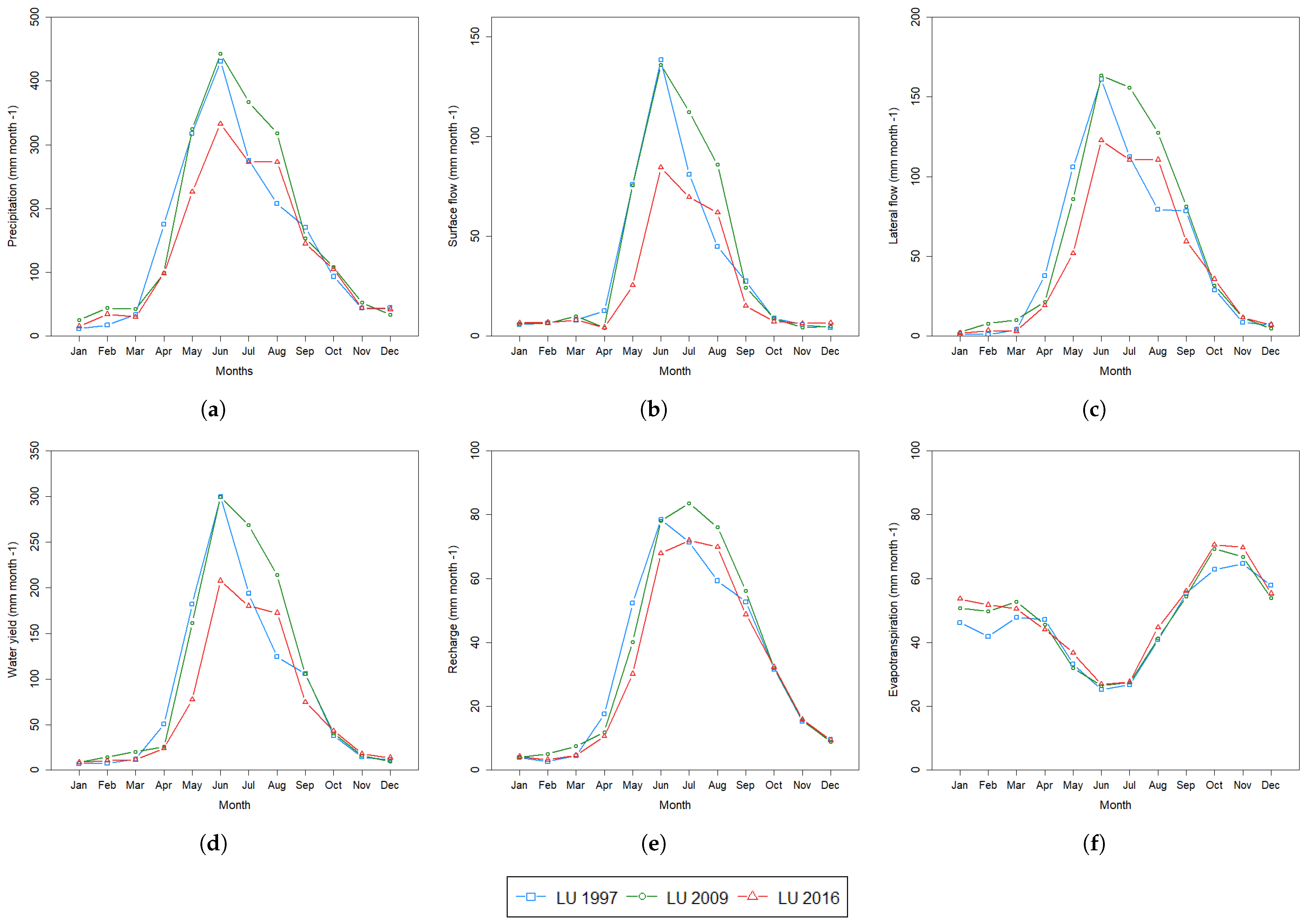
The changes on the monthly scale can be found in Figure 5 and Table 8. Differences in monthly precipitation (PRECIP) have been simulated during the period 1990–2019. In particular the lowest values were observed under LU 2016. The most determinant changes during the period 1990–1999 and 2010–2019 are related to a reduction of rainfall during the months between March to July, while an increase in precipitations has been estimated during the months of January and February. In accordance with precipitation changes, a reduction in surface flow (SURQ) with an accumulated decrease during the May to July period (116.2 mm) and an increase from November to March period (19.1 mm) was simulated. As a result, there was a reduction of 117.6 mm of annual accumulated SURQ values between LU 1997 and LU 2016. In the case of lateral flow (LATQ), some differences have been simulated for each month considering reductions and increases, in line with the changes in SURQ. Therefore, water yield (WY) decreased during the same months as SURQ and LATQ. In the case of groundwater recharge (RCHRG), and similarly with the behavior of other parameters, a reduction was achieved for the period 2010–2019 under LU 2016 configuration. For evapotranspiration (ET), a systematic increase has been simulated for the monthly study period between LU 1997 and LU 2016, and an accumulated ET value of 43 mm, with exception of the months of April and December with reduction of 5.6 mm.
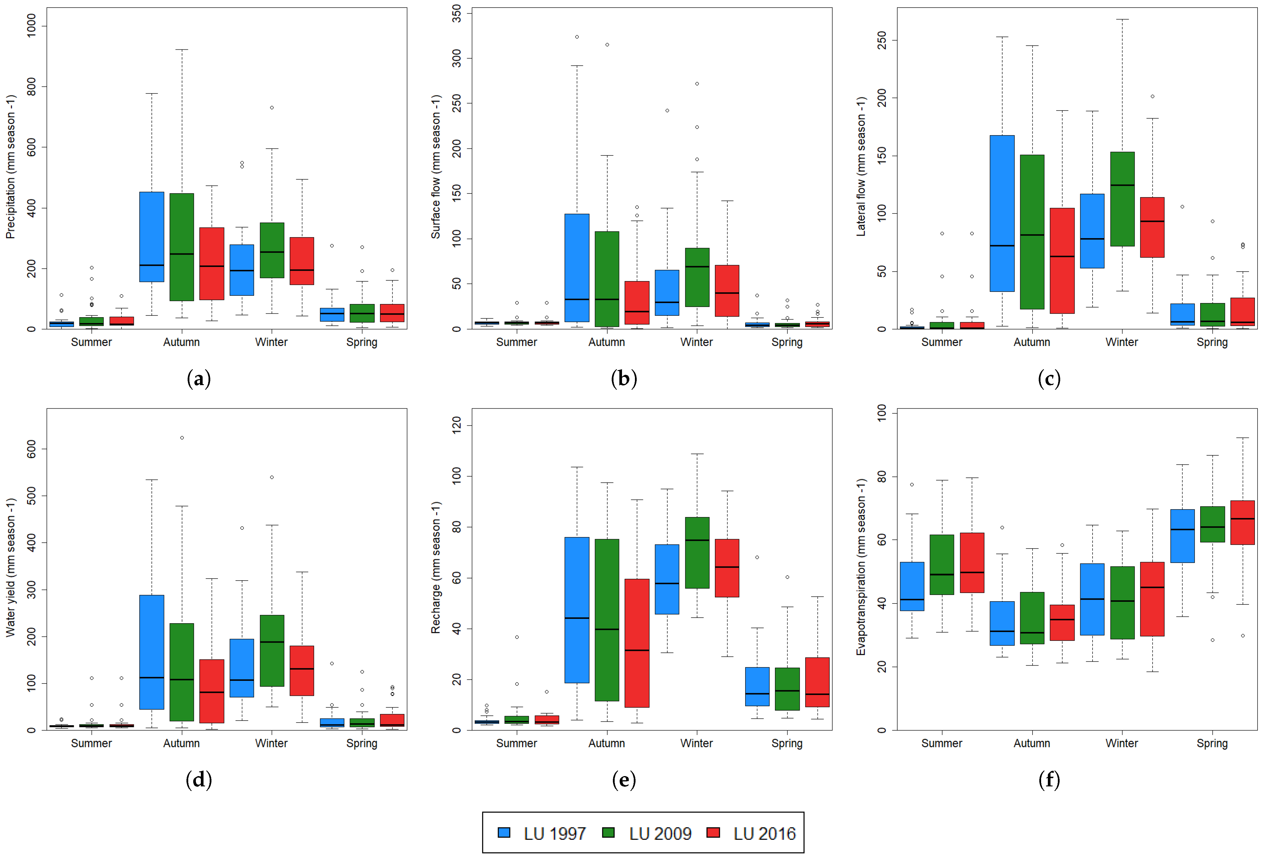
For evaluation on a seasonal scale (Figure 6), the seasons were defined as Summer (January, February, March), Autumn (April, May, June), Winter (July, August, September), and Spring (October, November, December).
Variations of PRECIP in the autumn and winter periods were achieved over the decades of study. Particularly, the variations increased in the amount of rainfall from 2000 to 2009 and decreased from 2010 to 2019. In the case of SURQ, a constant reduction was estimated during the study period. In particular with LU 2016, a strong reduction of surface flow during the autumn season (April–June) was estimated. In addition with a reduction during the last 10 years in comparison with LU 2009. Similar results were obtained for LATQ with a decrease during the last decade under LU 2016. In consequence, reductions on the resulting WY during autumn and winter seasons with LU 2016, in comparison with LU 1997 and 2009. Similarly, groundwater recharge (RCHRG) shows a tendency to reduce the amount during the autumn season. In the case of ET, summer values are higher under LU 2009 and 2016. During the winter and spring seasons, a partial increase under LU 2016 was simulated.
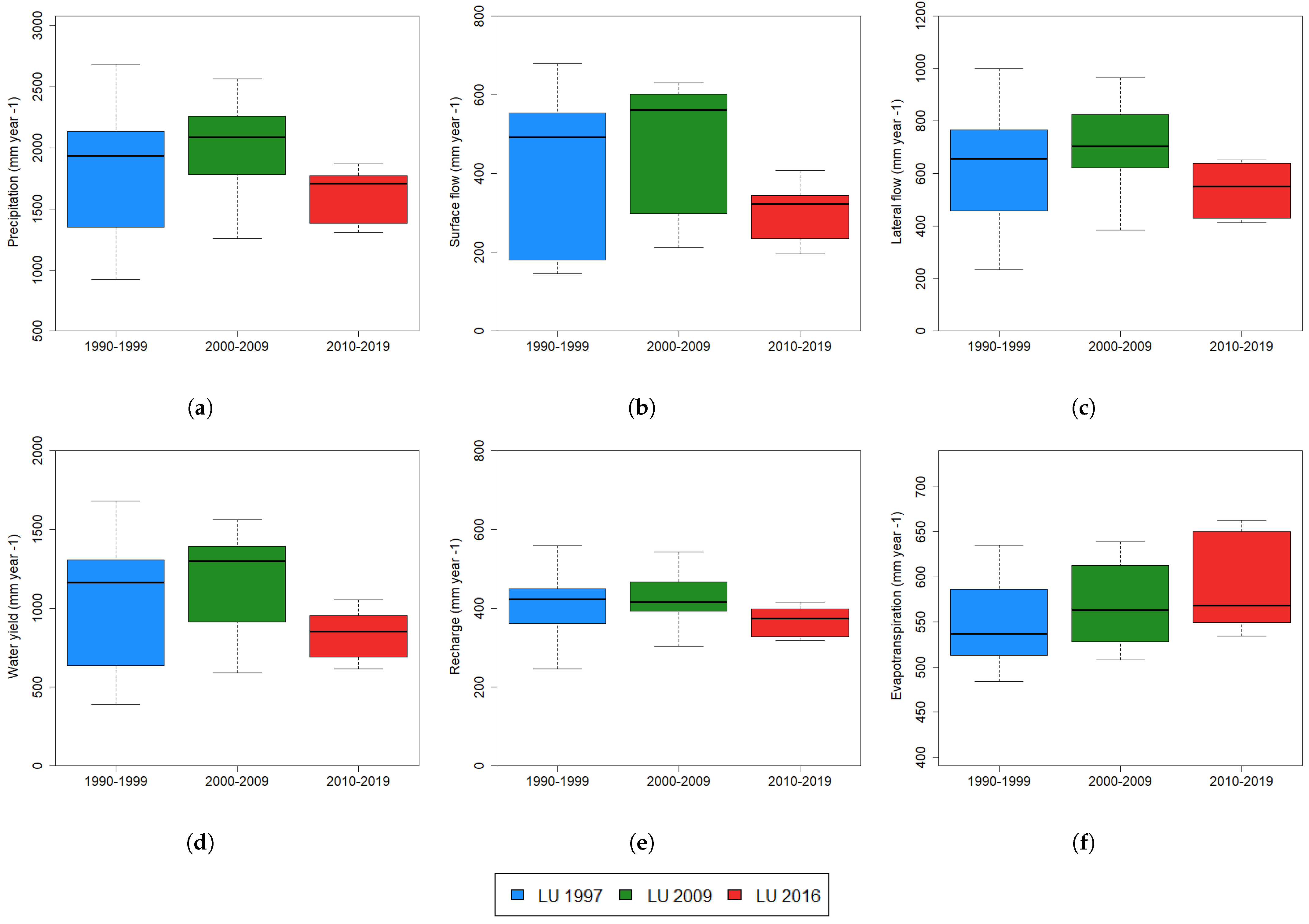
In the case of annual changes (Figure 7, Table 9), variation in precipitation values has been simulated during the three decades of study, particularly a major reduction was estimated in the last decade. In the decade of 2000–2009, an increase in PRECIP has been obtained in comparison to LU 1997; specifically, an accumulated yearly average value of 2010.2 mm is the maximum value for all the studied periods. Similarly, maximum values of SURQ, LATQ, WY, and RCHRG were obtained during the period with LU 2009.
The minimum accumulated yearly mean value for precipitation was obtained during the period 2010–2019 with LU 2016. In addition, the coefficient of variation is shorter during the last period, this indicates that the variability in rainfall amount has been lower in the last decade. In addition, a notorious reduction in the hydrological fluxes SURQ, LATQ, WY, and RCHRG emerges from simulations performed during the last decade of this study. Conversely, the higher yearly mean value of the ET flux was obtained with LU 2016.
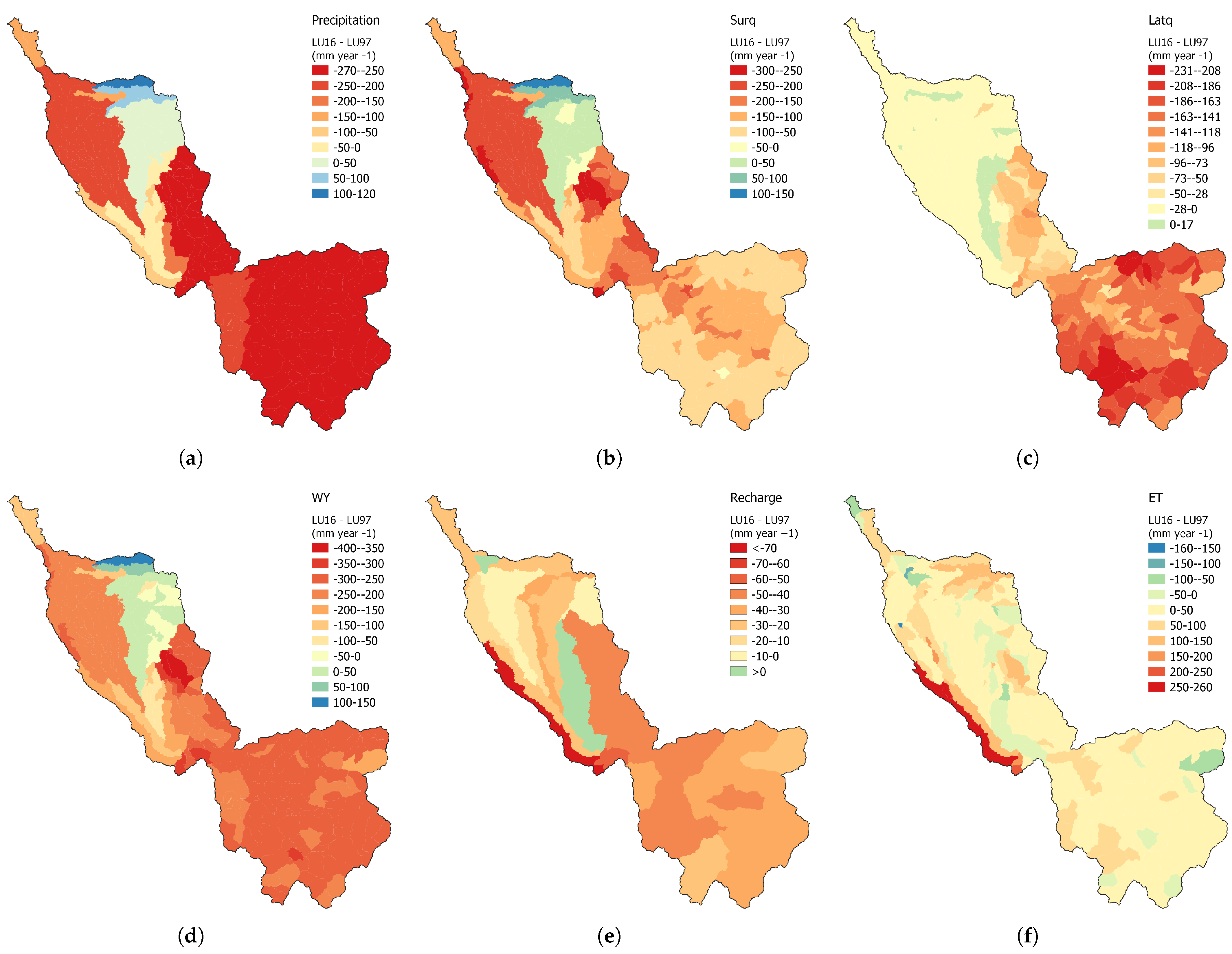
At the basin level (Figure 8), the differences between periods under LU 1997 and LU 2016 occurred synchronously with a drastic decrease in precipitation, especially in the mountainous part of the catchment. As to be expected, this leads to a reduction in the amount of SURQ in the middle part and at the outlet of the catchment. While a decrease in LATQ has been calculated in the middle part of the watershed in addition to the mountain part of the catchment. As consequence, reduction of water yield was simulated in different areas of the catchment. Similarly, RCHRG shows a tendency to decrease during the study period. Moreover, an increase in evapotranspiration has been calculated for some areas of the catchment, particularly in areas affected by land use changes related to shrubland reduction, increases in agricultural areas, and the expansion of pine tree plantations. The water extraction to supply the irrigation demand in the agricultural areas has increased during the last decades, contributing to a decrease in surface flow, water yield, and groundwater recharge, in addition to increases in evapotranspiration have been simulated in areas with crops of the catchment. Thus, for groundwater recharge and evapotranspiration, the strongest changes are to be expected mostly by remotion of shrublands and the establishment of pine trees and agricultural crops.

4. Discussion

4.1. SWAT+ Model Results

SWAT+ is a new and restructured version of the original SWAT, a broadly accepted and used tool for the small watershed to river basin-scale modeling. In relation to the complexity of the input parameters, for our study case, the software showed some restrictions, specifically concerning the meteorological input. The CAMELS-CL data set [39] was selected as the most suitable regional-scale input data set. However, due to some gaps in the data records, especially discharge, flow rate values can be underestimated. Other authors have also described analogous situations of poor peak estimation using different hydro-meteorological data, for example the CHIRPS database, which they attribute to systematic overestimation of precipitation in the mountain areas of Chile [35,52]. Nevertheless, it was possible to obtain satisfactory results with CAMELS-CL in terms of calibration and validation with the LU 1997, and, therefore, with the validation of LU 2009 and LU 2016 land covers. This supported our decision to evaluate the impacts of land use change on the hydrology of the catchment using the CAMELS-CL dataset. However, some runoff peaks in the observed data for both El Castillo and Quiriquina stations were very difficult to model adequately, a fact that we attribute to an overestimation of discharge at these stations.

4.2. Model Efficiency Criteria

Model performance was evaluated under different efficiency criteria following recommended ranges of values at a daily time step. The model was successfully calibrated and validated under the land use map of 1997. In addition, the model output coherence was successfully validated under LU 2009 and LU 2016. Following the recommendations of Moriasi et al. [49], R2 at daily time step can be considered satisfactory with values >0.5, at the contrary to monthly time step where the satisfactory qualification is achieved with values >0.7. Therefore, R2 values were considered satisfactory and good for the evaluated periods even with unreliable discharge peaks and gaps in observed data. Similarly, NSE values were encouraging for all cases, even with the gaps in observed data. In the case of rNSE, an useful efficiency criteria under data scarcity conditions [51], even with the inclusion of some unreliable runoff peaks, rNSE values were classified as satisfactory, good, and very good. Unlike NSE, rNSE calculation includes observed means ( Q ¯ o b s ) and ignores the gaps in observed data, thus, leading to higher indicator values. In the case of PBIAS, unsatisfactory results were calculated for all cases, possibly due to the short-term period of available data, in addition to the unreliable peak runoff values and some gaps from observed discharge data. The underestimation of discharge peaks, on the other hand, could be explained by different factors, like lack of snow measurement stations in the catchment, measurement errors, or heterogeneity of the hydro-meteorological data, particularly due to the complex geomorphology of mountain areas. Additionally, unreliable peak events have been reported in observed discharges for other catchments in Chile [33,35]. However, we calculate the PBIAS parameter using values in daily time steps, in contrast to other studies that use seasonal, monthly, or yearly values [49,50,53]. Therefore, the classification can be overestimated and the impact of the time-step choice becomes more relevant, particularly in data-poor regions.

4.3. Impacts of the LUC on the Catchment Hydrology

In addition to the evident combined effect of precipitations and LUC on surface runoff during the study period, it is important to mention that the changes in the remaining hydrological fluxes can also be influenced by different factors. This was explained by Yin et al. [54], who emphasized that in addition to climate parameters, other controlling factors, such as the total number and the spatial arrangement of SWAT+ Hydrological Response Units (HRUs) as basic spatial modeling entities, may also impact certain basin-internal hydrological fluxes like surface runoff. For instance, the change of spatial resolution of the model by increasing the number of HRUs for each land use map, by simultaneously leaving other parameters unchanged, leads to a potential increase in surface runoff [55]. This indicates that such type of change in model structure can affect the simulated water yield and streamflow estimation by the model. Over our chosen study period, a maximum number of 589 HRUs was reached for the Longaví by QSWAT+ by changing the land use map from LU 1997 to LU 2016. As confirmed by other researchers [55,56], the model is clearly sensitive to the number and arrangement of HRUs for a particular catchment. However, contrary to the findings of Her et al. [55], runoff and other hydrological fluxes decreased in our application from 2010 to 2019, even with the new configuration of 589 HRUs. Therefore, to keep the number of HRUs steady and not affect the water fluxes, the use of decision tables implemented in SWAT+ for the development of land use scenarios seems to be an alternative approach to configure SWAT+ dynamically [40]. Based on our experience, additional studies on the development of procedures for the evaluation of land use scenarios with SWAT+ are recommended, especially in data-poor areas subject to continuous land use changes due to varying agricultural practices and forestry production.
Together with decreases in precipitation, our modeling results further suggest that the land use changes related to the expansion of mixed forest and pine tree areas at the expense of shrubland and agricultural areas contribute to an overall alteration of water redistribution in the catchment, by affecting groundwater recharge and evapotranspiration. Such redistribution shifts further in the future. Under past and current management practices related to deforestation, where the fragmentation of native forests and a decrease in patch density have been steadily increasing across Central Chile [57], the scenario is not encouraging. In addition, a decline in precipitation, associated with an artificial increase in evapotranspiration due to land use changes during the last 30 years, may have led to a net decrease in surface flow, lateral flow, and overall catchment water yield, as suggested by the SWAT+ simulations. A very similar trend has also been observed by Martínez-Retureta et al. [35], who observed annual increases in ET, and a decrease in water yield on Chilean coastal basins in conjunction with exotic tree plantations.
It is known that mountain ecosystems are characterized by particular natural regulatory functions [58], especially in areas with forested landscapes, by controlling the local climate [59], and water quantity and quality. The climate regulation and provision of clean water on the local scale can be affected through land use changes by disturbing the equilibrium of the local micro-climate by changing variables such as evapotranspiration, surface runoff, or groundwater recharge. In the Longaví catchment, a clear decrease in groundwater recharge has been reproduced by SWAT+ simulations during the last decade, in particular under the LU 2016 land use scenario. It is known that the impacts of aquifer exploitation can decrease water availability [60]. As a consequence, it is necessary to pay attention to unsustainable groundwater use to avoid problems related to (drinking) water scarcity in the future. Therefore, it is imperative to implement a comprehensive regulatory system that considers current climatic conditions and territorial needs. Additionally, policies and institutions for the protection of natural ecosystems need to be reinforced, with a clear emphasis on ecosystem services, such as the natural regulation of water flows and the protection of its quality, as well as environmental governance under conditions of an uncertain future climate.
Although unsustainable water use is not apparent, collateral long-term consequences are foreseeable and include progressive ground and surface water depletion. Moreover, the reduction of surface flow can affect the future transfer of water from the Longaví catchment to the Digua dam through inter-basin water transfer. Improvements in discharge measurements are necessary to avoid unreliable runoff peaks and gaps in the time series. In addition, there is a lack of snow measuring points in mountain areas; therefore, we highlight the importance of continuing to support the development and maintenance of hydro-meteorological and discharge stations in Chile. The actual quantification of precipitation decline due to climate change and the quantification of intrinsic uncertainties of the climate change projections for the region are a matter of ongoing investigation.

5. Conclusions

The paper presents the results of a study aimed at quantifying the combined effect of precipitation and the influence of three consecutive decades of land use changes in the hydrology of Longaví catchment, central Chile. Three land use maps of the basin were jointly used to track the progressive transition from predominantly native vegetation toward intensive agricultural and forestry exploitation. The catchment hydrology was analyzed by simulating hydrological fluxes with the agro-hydrological model SWAT+. The model was calibrated and validated using daily discharge records. Noticeable alterations of the catchment hydrology by combined effects of the decline in precipitation together with land use transitions have been changing the partitioning of surface flow, lateral flow, groundwater recharge, and evapotranspiration. As a result, the overall catchment water balance is altered after each new land use configuration. The principal changes in land use occurred through the expansion of areas devoted to urban sprawl, crop plantations, forestry, and pine tree production. These modifications combined with decreases in precipitation, caused negative trends in surface flow and hence a progressive decline in mean annual water yield between 2000 and 2019. The study confirms that land use transition has progressively affected internal water redistribution, with strongest impacts on groundwater recharge and evapotranspiration. In this context, it is important to consider the potential long-term effects of agriculture, forest, and pine tree production as important factors that have the potential to affect not only the hydrology in the Longaví catchment but also that of neighboring basins in the future due to inter-basin transfers. Further studies related to the potential effects of climate change on the region are a matter of ongoing research.

Author Contributions

Conceptualization, H.M., I.A. and P.R.; methodology, H.M. and I.A.; software, H.M.; validation, H.M. and I.A.; formal analysis, H.M.; investigation, H.M.; resources, H.M., I.A. and P.R.; data curation, H.M.; writing—original draft preparation, H.M.; writing—review and editing, H.M., I.A., C.H. and P.R.; visualization, H.M.; supervision, I.A., C.H. and P.R.; project administration, I.A. and P.R.; funding acquisition, I.A., C.H. and P.R. All authors have read and agreed to the published version of the manuscript.

Funding

This research was funded by Bundesministerium für Bildung und Forschung (BMBF) Project no. 01DN17041.

Institutional Review Board Statement

Not applicable.

Informed Consent Statement

Not applicable.

Data Availability Statement

Not applicable.

Acknowledgments

We acknowledge the Bundesministerium für Bildung und Forschung (BMBF) for the financial support provided to the Project through Grant no. 01DN17041. The authors are also grateful to the Laboratory of Soil and Foliar Analysis of Pontificia Universidad Católica de Valparaíso (PUCV) for its support in performing soil sample analysis for the Longaví catchment.

Conflicts of Interest

The authors declare no conflict of interest. The funders had no role in the design of the study; in the collection, analyses, or interpretation of data; in the writing of the manuscript; or in the decision to publish the results.

Abbreviations

The following abbreviations are used in this manuscript:
SWAT+Soil and water assessment tool +
CIRENNatural Resources Information Center
CONAFNational Forest Corporation
CAMELS-CLCatchment Attributes and Meteorology for Large-sample Studies-Chile dataset
LULand Use
LUCLand Use Changes
SWSoil Water Content
PrPrecipitation
SurqSurface runoff
LatqLateral subsurface flow
ETEvapotranspiration
PercPercolation
FloReturn Flow
RchrgRecharge to deep aquifer
RevapPlant water uptake and evaporation
WYWater Yield
DEMDigital elevation model
HRUHydrological Response Unit
PETPotential evapotranspiration
SRTMShuttle Radar Topography Mission
DGACentral Water Directorate
BDBulk Density
CBNSoil Carbon Content
KSaturated Hydraulic Conductivity
PUCVPontificia Universidad Católica de Valparaíso
CN2SCS runoff curve number
ELEVElevation of weather station
EPCOPlant uptake compensation factor
ESCOSoil evaporation compensation factor
PERCOPercolation coefficient
SLOPELand surface slope
LAT_TTIMELateral flow travel time
ALPHABaseflow alpha factor
FLO_MINMinimum aquifer storage to allow return flow
REVAP_COGroundwater “revap” coefficient
REVAP_MINThreshold depth of water in the shallow aquifer for “revap” to occur
SURLAGSurface runoff lag time
TRNSRCHFraction of transmission losses from main channel that enter deep aquifer
ALBMoist soil albedo
ZDepth from soil surface to bottom of layer
NSENash-Sutcliffe Efficiency
rNSERelative Nash-Sutcliffe Efficiency
RMSERoot mean square error
RSRRMSE observations standard deviation ratio
PBIASPercent of model BIAS
R2Coefficient of determination
STDEVStandard Deviation
CVCoefficient of variation

References

  1. Turner, B.L.; Lambin, E.F.; Reenberg, A. The emergence of land change science for global environmental change and sustainability. Proc. Natl. Acad. Sci. USA 2007, 104, 20666–20671. [Google Scholar] [CrossRef] [PubMed]
  2. Barría, P.; Rojas, M.; Moraga, P.; Muñoz, A.; Bozkurt, D.; Alvarez-Garreton, C. Anthropocene and streamflow: Long-term perspective of streamflow variability and water rights. Elem. Sci. Anth. 2019, 7, 2. [Google Scholar] [CrossRef]
  3. DeFries, R.; Eshleman, K.N. Land-use change and hydrologic processes: A major focus for the future. Hydrol. Process. 2004, 18, 2183–2186. [Google Scholar] [CrossRef]
  4. He, M.; Hogue, T.S. Integrating hydrologic modeling and land use projections for evaluation of hydrologic response and regional water supply impacts in semi-arid environments. Environ. Earth Sci. 2012, 65, 1671–1685. [Google Scholar] [CrossRef]
  5. Sterling, S.M.; Ducharne, A.; Polcher, J. The impact of global land-cover change on the terrestrial water cycle. Nat. Clim. Chang. 2013, 3, 385–390. [Google Scholar] [CrossRef]
  6. Soto-Schönherr, S.; Iroumé, A. How much water do Chilean forests use? A review of interception losses in forest plot studies. Hydrol. Process. 2016, 30, 4674–4686. [Google Scholar] [CrossRef]
  7. Yan, W.; Deng, X.; Chen, X.; Tian, D.; Xiang, W.; Peng, Y. Long-term variations of rainfall interception in different growth stages of Chinese fir plantations. Hydrol. Sci. J. 2015, 60, 2178–2188. [Google Scholar] [CrossRef]
  8. Bronstert, A.; Niehoff, D.; Brger, G. Effects of climate and land-use change on storm runoff generation: Present knowledge and modelling capabilities. Hydrol. Process. 2002, 16, 509–529. [Google Scholar] [CrossRef]
  9. Ebling, É.; Reichert, J.M.; Peláez, J.J.Z.; Rodrigues, M.F.; Valente, M.L.; Lopes Cavalcante, R.B.; Reggiani, P.; Sirinivasan, R. Event-based hydrology and sedimentation in paired watersheds under commercial Eucalyptus and grasslands in the Brazilian Pampa biome. Int. Soil Water Conserv. Res. 2020, 9, 180–194. [Google Scholar] [CrossRef]
  10. Curtis, C.A.; Pasquarella, V.J.; Bradley, B.A. Landscape characteristics of non-native pine plantations and invasions in Southern Chile. Austral Ecol. 2019, 44, 1213–1224. [Google Scholar] [CrossRef]
  11. Locher-Krause, K.E.; Volk, M.; Waske, B.; Thonfeld, F.; Lautenbach, S. Expanding temporal resolution in landscape transformations: Insights from a landsat-based case study in Southern Chile. Ecol. Indic. 2017, 75, 132–144. [Google Scholar] [CrossRef]
  12. Andersson, K.; Lawrence, D.; Zavaleta, J.; Guariguata, M.R. More Trees, More Poverty? The Socioeconomic Effects of Tree Plantations in Chile, 2001–2011. Environ. Manag. 2016, 57, 123–136. [Google Scholar] [CrossRef] [PubMed]
  13. Manuschevich, D.; Sarricolea, P.; Galleguillos, M. Integrating socio-ecological dynamics into land use policy outcomes: A spatial scenario approach for native forest conservation in south-central Chile. Land Use Policy 2019, 84, 31–42. [Google Scholar] [CrossRef]
  14. Martínez Martínez, Y.; Goecke Coll, D.; Aguayo, M.; Casas-Ledón, Y. Effects of landcover changes on net primary production (NPP)-based exergy in south-central of Chile. Appl. Geogr. 2019, 113, 102101. [Google Scholar] [CrossRef]
  15. Echeverría, C.; Coomes, D.A.; Hall, M.; Newton, A.C. Spatially explicit models to analyze forest loss and fragmentation between 1976 and 2020 in southern Chile. Ecol. Modell. 2008, 212, 439–449. [Google Scholar] [CrossRef]
  16. Nahuelhual, L.; Carmona, A.; Lara, A.; Echeverría, C.; González, M.E. Land-cover change to forest plantations: Proximate causes and implications for the landscape in south-central Chile. Landsc. Urban Plan. 2012, 107, 12–20. [Google Scholar] [CrossRef]
  17. Aitken, D.; Rivera, D.; Godoy-Faúndez, A.; Holzapfel, E. Water scarcity and the impact of the mining and agricultural sectors in Chile. Sustainability 2016, 8, 128. [Google Scholar] [CrossRef]
  18. Garreaud, R.D.; Alvarez-Garreton, C.; Barichivich, J.; Pablo Boisier, J.; Christie, D.; Galleguillos, M.; LeQuesne, C.; McPhee, J.; Zambrano-Bigiarini, M. The 2010–2015 megadrought in central Chile: Impacts on regional hydroclimate and vegetation. Hydrol. Earth Syst. Sci. 2017, 21, 6307–6327. [Google Scholar] [CrossRef]
  19. Valdés-Pineda, R.; Pizarro, R.; García-Chevesich, P.; Valdés, J.B.; Olivares, C.; Vera, M.; Balocchi, F.; Pérez, F.; Vallejos, C.; Fuentes, R.; et al. Water governance in Chile: Availability, management and climate change. J. Hydrol. 2014, 519, 2538–2567. [Google Scholar] [CrossRef]
  20. Rivera, D.; Godoy-Faúndez, A.; Lillo, M.; Alvez, A.; Delgado, V.; Gonzalo-Martín, C.; Menasalvas, E.; Costumero, R.; García-Pedrero, Á. Legal disputes as a proxy for regional conflicts over water rights in Chile. J. Hydrol. 2016, 535, 36–45. [Google Scholar] [CrossRef]
  21. Muñoz, A.A.; Klock-Barría, K.; Alvarez-Garreton, C.; Aguilera-Betti, I.; González-Reyes, A.; Lastra, J.; Chávez, R.; Barría, P.; Christie, D.; Rojas-Badilla, M.; et al. Water crisis in petorca basin, Chile: The combined effects of a mega-drought and water management. Water 2020, 12, 648. [Google Scholar] [CrossRef]
  22. Breuer, L.; Huisman, J.A.; Willems, P.; Bormann, H.; Bronstert, A.; Croke, B.F.; Frede, H.G.; Gräff, T.; Hubrechts, L.; Jakeman, A.J.; et al. Assessing the impact of land use change on hydrology by ensemble modeling (LUCHEM). I: Model intercomparison with current land use. Adv. Water Resour. 2009, 32, 129–146. [Google Scholar] [CrossRef]
  23. Dwarakish, G.; Ganasri, B. Impact of land use change on hydrological systems: A review of current modeling approaches. Cogent Geosci. 2015, 1, 1115691. [Google Scholar] [CrossRef]
  24. Lahmer, W.; Pfützner, B.; Becker, A. Assessment of land use and climate change impacts on the mesoscale. Phys. Chem. Earth 2001, 26, 565–575. [Google Scholar] [CrossRef]
  25. Klöcking, B.; Ströbl, B.; Knoblauch, S.; Maier, U.; Pfützner, B.; Gericke, A. Development and allocation of land-use scenarios in agriculture for hydrological impact studies. Phys. Chem. Earth 2003, 28, 1311–1321. [Google Scholar] [CrossRef]
  26. Arnold, J.G.; Srinivasan, R.; Muttiah, R.S.; Williams, J.R. Large Area Hydrologic Modeling and Assessment Part I: Model Development. J. Am. Water Resour. Assoc. 1998, 34, 73–89. [Google Scholar] [CrossRef]
  27. Bieger, K.; Arnold, J.G.; Rathjens, H.; White, M.J.; Bosch, D.D.; Allen, P.M. Representing the Connectivity of Upland Areas to Floodplains and Streams in SWAT+. J. Am. Water Resour. Assoc. 2019, 55, 578–590. [Google Scholar] [CrossRef]
  28. Bieger, K.; Arnold, J.; Rathjens, H.; White, M.; Bosch, D.; Allen, P.; Volk, M.; Srinivasan, R. Introduction to SWAT+, a completely restructured version of the Soil and Water Assessment Tool. J. Am. Water Resour. Assoc. 2017, 53, 115–130. [Google Scholar] [CrossRef]
  29. Musie, M.; Sen, S.; Chaubey, I. Hydrologic responses to climate variability and human activities in Lake Ziway Basin, Ethiopia. Water 2020, 12, 164. [Google Scholar] [CrossRef]
  30. Nasiri, S.; Ansari, H.; Ziaei, A.N. Simulation of water balance equation components using SWAT model in Samalqan Watershed (Iran). Arab. J. Geosci. 2020, 13, 421. [Google Scholar] [CrossRef]
  31. Nkwasa, A.; Chawanda, C.J.; Msigwa, A.; Komakech, H.C.; Verbeiren, B.; van Griensven, A. How can we represent seasonal land use dynamics in SWAT and SWAT+ models for African cultivated catchments. Water 2020, 12, 1541. [Google Scholar] [CrossRef]
  32. Stehr, A.; Debels, P.; Romero, F.; Alcayaga, H. Hydrological modelling with SWAT under conditions of limited data availability: Evaluation of results from a Chilean case study. Hydrol. Sci. J. 2008, 53, 588–601. [Google Scholar] [CrossRef]
  33. Stehr, A.; Aguayo, M.; Link, O.; Parra, O.; Romero, F.; Alcayaga, H. Modelling the hydrologic response of a mesoscale Andean watershed to changes in land use patterns for environmental planning. Hydrol. Earth Syst. Sci. 2010, 14, 1963–1977. [Google Scholar] [CrossRef]
  34. Uniyal, B.; Dietrich, J.; Vu, N.Q.; Jha, M.K.; Arumí, J.L. Simulation of regional irrigation requirement with SWAT in different agro-climatic zones driven by observed climate and two reanalysis datasets. Sci. Total Environ. 2019, 649, 846–865. [Google Scholar] [CrossRef]
  35. Martínez-Retureta, R.; Aguayo, M.; Stehr, A.; Sauvage, S.; Echeverría, C.; Sánchez-Pérez, J. Effect of land use/cover change on the hydrological response of a southern center basin of Chile. Water 2020, 12, 302. [Google Scholar] [CrossRef]
  36. Omani, N.; Srinivasan, R.; Karthikeyan, R.; Venkata Reddy, K.; Smith, P.K. Impacts of climate change on the glacier melt runoff from five river basins. Trans. ASABE 2016, 59, 829–848. [Google Scholar] [CrossRef]
  37. Omani, N.; Srinivasan, R.; Karthikeyan, R.; Smith, P.K. Hydrological modeling of highly glacierized basins (Andes, Alps, and Central Asia). Water 2017, 9, 111. [Google Scholar] [CrossRef]
  38. SERNAGEOMIN. Servicio Nacional de Geología y Minería. Mapa Geológico de Chile: Versión Digital. Publicación Geológica Digital, No. 4. 2003. Available online: http://www.ipgp.fr/~dechabal/Geol-millon.pdf (accessed on 20 July 2022).
  39. Alvarez-Garreton, C.; Mendoza, P.A.; Boisier, J.P.; Addor, N.; Galleguillos, M.; Zambrano-Bigiarini, M.; Lara, A.; Puelma, C.; Cortes, G.; Garreaud, R.; et al. The CAMELS-CL dataset: Catchment attributes and meteorology for large sample studies—Chile dataset. Hydrol. Earth Syst. Sci. 2018, 22, 5817–5846. [Google Scholar] [CrossRef]
  40. Arnold, J.G.; Bieger, K.; White, M.J.; Srinivasan, R.; Dunbar, J.A.; Allen, P.M. Use of decision tables to simulate management in SWAT+. Water 2018, 10, 713. [Google Scholar] [CrossRef]
  41. Dile, Y.; Srinivasan, R.; George, C. QGIS Interface for SWAT+: QSWAT+. 2021. Available online: https://docplayer.net/204909159-Qgis-interface-for-swat-qswat.html (accessed on 20 July 2022).
  42. Jarvis, A.; Reuter, H.I.; Nelson, A.; Guevara, E. Hole-Filled Seamless SRTM Data V4, International Centre for Tropical Agriculture (CIAT). CIAT. 2008. Available online: http://srtm.csi.cgiar.org (accessed on 20 July 2022).
  43. CIREN. Estudio Agrológico VII Región. Descripción de Suelos, Materiales y Símbolos; Centro de Información de Recursos Naturales: Santiago, Chile, 1997; pp. 1–660. [Google Scholar]
  44. CONAF. Catastro de Uso del Suelo y Vegetación. Monitoreo y Actualización en la VII Región del Maule. Corporacion Nacional Forestal. 2016. Available online: https://sit.conaf.cl/ (accessed on 20 July 2022).
  45. Molina, A.; Falvey, M.; Rondanelli, R. A solar radiation database for Chile. Sci. Rep. 2017, 7, 14823. [Google Scholar] [CrossRef] [Green Version]
  46. Yen, H.; Park, S.; Arnold, J.G.; Srinivasan, R.; Chawanda, C.J.; Wang, R.; Feng, Q.; Wu, J.; Miao, C.; Bieger, K.; et al. IPEAT+: A Built-In Optimization and Automatic Calibration Tool of SWAT+. Water 2019, 11, 1681. [Google Scholar] [CrossRef]
  47. Abbaspour, K.C.; Vaghefi, S.A.; Srinivasan, R. A guideline for successful calibration and uncertainty analysis for soil and water assessment: A review of papers from the 2016 international SWAT conference. Water 2017, 10, 6. [Google Scholar] [CrossRef]
  48. Krause, P.; Boyle, D.; Bäse, F. Comparison of Different Efficiency Criteria for Hydrologic Models. Adv. Geosci. 2005, 5, 89–97. [Google Scholar] [CrossRef]
  49. Moriasi, D.N.; Gitau, M.W.; Pai, N.; Daggupati, P. Hydrologic and water quality models: Performance measures and evaluation criteria. Trans. ASABE 2015, 58, 1763–1785. [Google Scholar] [CrossRef]
  50. Moriasi, D.; Arnold, J.; Van Liew, M.; Bingner, R.; Harmel, R.; Veith, T. Model Evaluation Guidelines for Systematic Quantification of Accuracy in Watershed Simulations. Trans. ASABE 2007, 50, 885–900. [Google Scholar] [CrossRef]
  51. González, V.G.; Colmenares, L.Á; Fidalgo, J.F.L.; Ruiz, G.R.; Bandera, C.F. Uncertainy’s indices assessment for calibrated energy models. Energies 2019, 12, 2096. [Google Scholar] [CrossRef]
  52. Zambrano, F.; Wardlow, B.; Tadesse, T. Evaluating satellite-derived long-term historical precipitation datasets for drought monitoring in Chile. Remote Sens. Agric. Ecosyst. Hydrol. XVIII 2016, 9998, 999823. [Google Scholar] [CrossRef]
  53. Gyamfi, C.; Ndambuki, J.M.; Salim, R.W. Hydrological responses to land use/cover changes in the Olifants Basin, South Africa. Water 2016, 8, 588. [Google Scholar] [CrossRef]
  54. Yin, J.; He, F.; Xiong, Y.J.; Qiu, G.Y. Effects of land use/land cover and climate changes on surface runoff in a semi-humid and semi-arid transition zone in northwest China. Hydrol. Earth Syst. Sci. 2017, 21, 183–196. [Google Scholar] [CrossRef]
  55. Her, Y.; Frankenberger, J.; Chaubey, I.; Srinivasan, R. Threshold effects in HRU definition of the soil and water assessment tool. Trans. ASABE 2015, 58, 367–378. [Google Scholar] [CrossRef]
  56. Pignotti, G.; Rathjens, H.; Cibin, R.; Chaubey, I.; Crawford, M. Comparative analysis of HRU and grid-based SWAT models. Water 2017, 9, 272. [Google Scholar] [CrossRef]
  57. Echeverria, C.; Coomes, D.; Salas, J.; Rey-Benayas, J.M.; Lara, A.; Newton, A. Rapid deforestation and fragmentation of Chilean Temperate Forests. Biol. Conserv. 2006, 130, 481–494. [Google Scholar] [CrossRef]
  58. Hu, A.; Wang, J.; Sun, H.; Niu, B.; Si, G.; Wang, J.; Yeh, C.F.; Zhu, X.; Lu, X.; Zhou, J.; et al. Mountain biodiversity and ecosystem functions: Interplay between geology and contemporary environments. ISME J. 2020, 14, 931–944. [Google Scholar] [CrossRef]
  59. Perera, A.H.; Peterson, U.; Martínez Pastur, G.; Iverson, L.R. Ecosystem Services from Forest Landscapes; Springer International Publishing: Cham, Switzerland, 2018; pp. 1–265. [Google Scholar]
  60. Turner, S.W.D.; Hejazi, M.; Yonkofski, C.; Kim, S.H.; Kyle, P. Influence of Groundwater Extraction Costs and Resource Depletion Limits on Simulated Global Nonrenewable Water Withdrawals Over the Twenty-First Century. Earth’s Future 2019, 7, 123–135. [Google Scholar] [CrossRef] [Green Version]
Figure 1. Localization of Longaví catchment.
Hydrology 09 00169 g001
Figure 2. (a) Slope map, (b) soil type map and (c) stations on the Longaví catchment.
Hydrology 09 00169 g002
Figure 3. Land use maps of 1997, 2009, and 2016.
Hydrology 09 00169 g003
Figure 4. Calibration (a) and validation (b) period at daily time step for El Castillo and Quiriquina stations, respectively.
Hydrology 09 00169 g004
Figure 5. Monthly average values for the studied periods with LU 1997 (1990–1999), LU 2009 (2000–2009), and LU 2016 (2010–2019) for the parameters: (a) Precipitation, (b) Surface flow, (c) Lateral flow, (d) Water yield, (e) Recharge, and (f) Evapotranspiration.
Hydrology 09 00169 g005
Figure 6. Seasonal average of the studied periods with LU 1997 (1990–1999), LU 2009 (2000–2009), and LU 2016 (2010–2019) for the parameters: (a) Precipitation, (b) Surface flow, (c) Lateral flow, (d) Water yield, (e) Recharge, and (f) Evapotranspiration.
Hydrology 09 00169 g006
Figure 7. Annual average by decades under LU 1997 (1990–1999), LU 2009 (2000–2009), and LU 2016 (2010–2019) for the parameters: (a) Precipitation, (b) Surface flow, (c) Lateral flow, (d) Water yield, (e) Recharge, and (f) Evapotranspiration.
Hydrology 09 00169 g007
Figure 8. Changes between 1990 and 2019 under LU 1997 and LU 2016 for the parameters: (a) Precipitation, (b) Surface flow, (c) Lateral flow, (d) Water yield, (e) Recharge and (f) Evapotranspiration.
Hydrology 09 00169 g008
Table 1. Input parameters used for SWAT+ modeling.
TypeInput DataDescriptionSource
Spatial DataDEMDigital elevation model (90 m resolution)Shuttle Radar Topography Mission [42]
Soil typeSoil Samples and Agrological study of El MauleField studies and CIREN 1997 [43]
Land useLand use maps 1997, 2009, 2016CONAF 2017 [44]
Meteorological DataTemperaturesMinimum and maximum daily temperatures (10 *)Camels-CL dataset [39]
PrecipitationDaily precipitation (10 *)Camels-CL dataset [39]
Wind velocityDaily wind (4 *)DGA
Relative HumidityDaily relative humidity (1 *)DGA
Solar radiationDaily solar radiation (5 *)Chilean Ministry of Energy [45]
* Number of stations selected.
Table 2. General description of the soils in the Longaví catchment.
SymbolNameLayersDepth (cm) *BD (g cm−3) *CBN (%) *K (mm hr−1) *pH *Texture *
ACHAchibueno312001.61.311.86.3Loam
APOAsociación Posillas311501.30.814.66.2Clay loam
SRBAsociación Sierra Bellavista38001.51.264.26.5Loamy sand
CLBCaliboro49001.70.519.67.2Loamy
CHIChiguay34501.61.316.35.8Clay loam
CBNColbun58501.51.19.95.9Silty clay
DIGDiguillin411001.14.242.66.4Loamy silt
LOBLa Obra38001.80.913.06.0Loamy sand
LNSLinares35001.51.717.16.8Loamy sand
MLCMaulecura25501.75.529.26.6Loamy
MRFMiraflores37501.70.527.87.2Loamy
MSEMiscelaneo estero37501.50.426.57.2Loamy
MSPMiscelaneo pantano37501.70.527.87.3Loamy
MRFMiscelaneo rio26001.31.429.25.8Loamy
PALPalmilla39501.90.722.86.7Clay loamy
PNDPanimavida39001.21.022.56.1Clay loam
PRLParral411201.60.519.66.2Clay loam
PUTPutagan38501.51.212.16.7Loamy sand
QLAQuella37001.50.714.66.6Clay
SVJSan Javier311001.60.716.76.2Loamy silt
VICVillaseca35001.81.614.07.0Clay loam
* Corroborated by field studies.
Table 3. Distribution of land uses for LU 1997, LU 2009, and LU 2016 by km2 and relative values (%).
Land UseArea (km2)Area (%)
LU 1997LU 2009LU 2016LU 1997LU 2009LU 2016
Urban3.110.710.70.220.770.77
Agriculture416.8391.0397.030.0428.1928.62
Wetlands0.00.10.20.000.010.01
Barren108.5108.4111.27.827.818.02
Water28.029.026.82.022.091.93
Pasture75.775.076.65.455.405.52
Mixed grassland/shrubland9.59.28.40.690.670.61
Shrubland109.382.374.67.885.945.38
Range brush58.549.646.44.223.573.34
Forest mixed378.4414.7415.527.2829.8929.95
Forest evergreen66.862.263.64.814.494.59
Pine tree132.8155.0156.59.5711.1711.28
Table 4. Parameters used for the sensitivity analysis of the model.
ParameterGroupDescriptionUnits
CN2HRUSCS runoff curve number-
ELEVHRUElevation of weather stationm
EPCOHRUPlant uptake compensation factor-
ESCOHRUSoil evaporation compensation factor-
PERCOHRUPercolation coefficientfraction
SLOPEHRULand surface slopem m−1
LAT_TTIMEHRULateral flow travel timedays
ALPHAAQUBaseflow alpha factor (days)days
FLO_MINAQUMinimum aquifer storage to allow return flowm
REVAP_COAQUGroundwater “revap” coefficient-
REVAP_MINAQUThreshold depth of water in the shallow aquifer for “revap” to occur (mm)m
SURLAGBSNSurface runoff lag timedays
TRNSRCHBSNFraction of transmission losses from main channel that enter deep aquiferfraction
ALBSOLMoist soil albedo-
KSOLSaturated hydraulic conductivitymm h−1
ZSOLDepth from soil surface to bottom of layermm
Table 5. Parameters used for the SWAT+ calibration model with SWAT+ Toolbox.
ParameterGroupDescriptionCalibration Values
MinimumMaximumAdjustedChange Type
CN2HRUSCS runoff curve number−5050−36.25% chg
EPCOHRUPlant uptake compensation factor−5050−48.85% chg
ESCOHRUSoil evaporation compensation factor−8010−78.03% chg
PERCOHRUPercolation coefficient−508079.21% chg
KSOLSaturated hydraulic conductivity−8020−72.08% chg
FLO_MINAQUMinimum aquifer storage to allow return flow−20608.85% chg
REVAP_MINAQUThreshold depth of water in the shallow aquifer for “revap” to occur−5010−21.28% chg
Table 6. Efficiency criteria for the period without calibration and calibration (1985–1986) and for the validation period (1996–1998) at daily time step for El Castillo and Quiriquina stations.
StatisticiansEl CastilloQuiriquina
Without CalibrationCalibrationValidationWithout CalibrationCalibrationValidation
R20.630.640.660.580.570.69
NSE0.560.530.640.510.500.64
rNSE0.810.870.700.750.830.61
RSR0.670.690.600.700.700.60
PBIAS−38.7−39.1−28.7−42.7−42.1−35.1
Table 7. Model efficiency criteria under LU 2009 (2006–2009) and LU 2016 (2012) at daily time step for El Castillo and Quiriquina stations.
StatisticiansEl CastilloQuiriquina
LU 2009LU 2016LU 2009LU 2016
R20.760.610.720.60
NSE0.660.560.640.57
rNSE0.780.830.660.61
RSR0.590.660.600.66
PBIAS−34.7−30.9−36.3−26.4
Table 8. Monthly average changes of PRECIP, SURQ, LATQ, WY, RCHRG, and ET from LU 1997 (1990–1999) and LU 2016 (2010–2019) on a daily scale. Values are expressed as mm month−1.
MonthPRECIPSURQLATQWYRCHRGET
199720161997201619972016199720161997201619972016
January11.415.35.96.71.21.87.08.54.14.346.353.7
February17.434.56.76.81.03.67.710.52.73.341.951.8
March34.329.98.18.24.23.212.311.34.54.747.950.5
April175.298.212.74.437.919.450.623.817.610.747.244.1
May317.8226.476.125.5106.051.9182.177.452.430.233.336.7
June430.8332.4138.684.6161.1122.8299.7207.478.467.825.326.9
July275.2272.681.169.6112.4110.5193.6180.171.371.926.827.7
August207.9272.944.962.079.4110.6124.3172.659.369.840.944.7
September170.6145.027.515.178.459.4105.974.652.748.855.456.0
October93.5105.09.17.429.035.738.143.131.732.362.870.5
November43.843.95.86.58.611.614.518.115.316.064.669.7
December44.642.24.36.67.07.111.313.89.69.457.855.3
Table 9. Annual average (Mean) and coefficient of variation (CV) by decades for PRECIP, SURQ, LATQ, WY, RCHRG, and ET under LU 1997, LU 2009, and LU 2016 for the studied period. Values are expressed as mm year−1 and %, respectively.
DecadePRECIPSURQLATQWYRCHRGET
MeanCVMeanCVMeanCVMeanCVMeanCVMeanCV
1990–19991822.529.8421.046.5626.236.61047.240.0399.522.8550.28.5
2000–20092010.219.6479.533.0704.425.31183.927.3419.215.6570.77.9
2010–20191618.413.2303.424.7537.717.5841.119.1369.19.8587.68.5
Publisher’s Note: MDPI stays neutral with regard to jurisdictional claims in published maps and institutional affiliations.

