The Seasonal Water Balance of Western-Juniper-Dominated and Big-Sagebrush-Dominated Watersheds

Abstract

The combined impacts of woody plant encroachment and climate variability have the potential to alter the water balance in many sagebrush steppe ecosystems in the Western USA, leading to reduced water availability in these already water-scarce regions. This study compared the water-balance characteristics of two adjacent semiarid watersheds in central Oregon, USA: one dominated by big sagebrush and one dominated by western juniper. Precipitation, springflow, streamflow, shallow groundwater levels, and soil moisture were measured. The potential evapotranspiration was calculated using the Hargreaves–Samani method. Potential evapotranspiration and a water-balance approach were used to calculate seasonal actual evapotranspiration. The shallow aquifer recharge was calculated using the Water-Table-Fluctuation-Method. Evapotranspiration, followed by deep percolation, accounted for the largest portion (83% to 86% of annual precipitation) of water output for both watersheds. Springflow and streamflow rates were generally greater at the sagebrush-dominated watershed. Snow-dominated years showed greater amounts of groundwater recharge and deep percolation than years where a larger portion of precipitation fell as rain, even when total annual precipitation amounts were similar. This study’s results highlight the role of vegetation dynamics, such as juniper encroachment, and seasonal precipitation characteristics, on water availability in semiarid rangeland ecosystems.

1. Introduction

Many areas of the Western US are facing severe drought conditions that have dramatically decreased the levels of water available for numerous production and ecological functions. Long-term deficits in available water associated with prolonged droughts and a changing climate threaten production systems and ecosystem resilience in many arid and semiarid regions worldwide. Reduced snowpack [1], shifts from snow to rain-dominated precipitation [2], and reduced groundwater recharge [3,4,5] can severely impact water availability for human and environmental use. Seasonal timing of precipitation is a key factor influencing the water balance, and therefore water availability, in sagebrush steppe ecosystems [6], particularly in regions with already variable precipitation patterns [7]. Shifts in plant functional types have also been shown to alter the water balance of dryland ecosystems [8]. In particular, the encroachment of juniper (Juniperus spp.) in sagebrush steppe ecosystems has been associated with altered flow regimes [9], earlier snowmelt and increased evapotranspiration [10], and increased overland flow and erosion [11]. In the sagebrush steppe ecosystems of the Great Basin, the combined effects of woody plant encroachment [10,12] and increased temperatures and precipitation variability associated with climate change [2,13] can alter the seasonal water balance.

A technique commonly used to assess water availability and the partitioning of water resources in a given area is the water-balance method (WBM). In the WBM, inflows (e.g., precipitation) offset outflows (e.g., runoff, evapotranspiration, and changes in soil water content). Some water budget components are relatively easy to measure (e.g., soil water content, precipitation, and runoff); other components, such as evapotranspiration, can be simulated based on available weather data. Evapotranspiration and deep percolation can also be calculated as the residual term, assuming all other components are known. The WBM approach has been used in a range of climates and ecosystems, such as sagebrush ecosystems [14], semiarid savannas [15], oak woodlands [16], and agricultural fields [17]. Additionally, the WBM has been used to examine climate change [3] and land-use practices [18]. This approach has also been used to examine a broad range of temporal scales, including long-term examination of the water balance [15,19,20] and short-term precipitation events [21]. Similarly, the WBM has been applied across spatial scales from the watershed [22] to the larger catchment and continent scales [23]. Several studies have examined the water balance of semiarid shrublands in the Southwestern USA [19,24,25] and other semiarid regions of the world [26,27,28,29].

The partitioning of the water-balance components is less known in the western juniper (Juniperus occidentalis) and sagebrush (Artemisia tridentata) dominated settings in the Pacific Northwest region of North America. Some research has focused on variables such as soil water content (e.g., see [30,31,32]), runoff (e.g., see [30]), and transpiration (e.g., see [32,33,34]). Limited research has been conducted into the evapotranspiration (ET) of western juniper and sagebrush steppe ecosystems. The measurement of ET poses unique challenges. Methods using eddy-covariance or Bowen Ratio systems have been successfully applied in many studies (e.g., see [35,36,37]), as well as direct measurements of evaporation, such as pan evaporation measurement (e.g., see [38]), or evapotranspiration, such as lysimeters [39], as well as sap flow approaches to measure transpiration (e.g., see [40]). However, the variation in ET across the landscape due to vegetation heterogeneity or topography cannot be captured without multiple monitoring systems, which are often costly or difficult to maintain in remote environments. Reference ET (ET₀) or potential evapotranspiration (PET), the amount of ET that would occur when moisture is not limited, is frequently used to estimate actual ET (ET_A). The Hargreaves–Samani equation [41] requires minimal climate data and has been successfully used to calculate PET in arid and semiarid regions [42,43]. Thornthwaite–Mather-type water-balance equations [44,45] have been used to estimate ET_A and other water-balance elements [46,47] and are particularly useful due to their simplicity and limited data requirements.

Surface water and groundwater interactions influence multiple ecological and hydrological relationships occurring in a landscape. Understanding these connections is critical for developing sound comprehensive resource management plans [48,49]. Surface water and groundwater cannot be seen as isolated components and are spatially and temporally variable in many systems [50]. In many instances, seasonal precipitation or irrigation inputs percolating below the effective rooting zone contribute to the replenishment of the shallow aquifer [30,51]. Groundwater recharge can be influenced by geologic characteristics, such as the presence of fractured bedrock or basalt [30,52], and precipitation timing and quantity [53] or vegetation [54].

Many rangeland ecosystems, including sagebrush and juniper woodlands, are not considered high water-yielding sources mainly because of the low precipitation and the high evapotranspiration losses associated with these landscapes. Long-term groundwater recharge is assumed to be minimal in some areas of the US Southwest region [25,53,55], where the bulk of the precipitation that falls in the hot summer generally corresponds to vegetation productivity, and consequently with high evapotranspiration rates. However, the recharge of the shallow aquifer can be significant in winter precipitation-dominated systems where there is limited consumptive use from vegetation. Aquifer replenishment in response to seasonal water inputs can be more significant in regions overlying shallow aquifers characterized by permeable soils that allow rapid water infiltration and aquifer recharge [30].

Groundwater recharge can be calculated by using different methods [56], including soil-water budgets [56,57], isotope measurements [58], Darcy’s equation [59], and groundwater-level fluctuations [60]. Similar to the WBM described above, soil-water-budget approaches require information about other water-balance characteristics, such as ET_A, that may not be readily available. The use of tracers can be challenging in environments where regular sampling and analysis of tracer concentrations in the groundwater may not be possible. The Water-Table-Fluctuation Method (WTFM) is a commonly used approach that calculates recharge in unconfined aquifers based on groundwater-level data [60]. The WTFM has been applied in several studies (e.g., see [61,62,63]) and is advantageous, particularly in data-limited environments, due to its simplicity.

It is increasingly recognized that woody vegetation expansion effects on hydrologic processes such as groundwater recharge must be better understood. While woody plant encroachment can influence groundwater recharge due to changes in infiltration rates, interception, and transpiration, among other factors, these impacts vary across spatial and temporal scales [64]. Moore et al. [65] found that removal of shrubs (primarily honey mesquite, Prosopis glandulosa) resulted in a slight increase in groundwater recharge at a study site in Southwest Texas; however, this varied with soil type and the amount of vegetation cover removed. Research addressing the effects of woody vegetation on water yield in cool climates is limited. Only a few studies (see, for example, [30,52]) have addressed vegetation and groundwater relationships in sagebrush- and juniper-dominated landscapes. More studies focused on the linkages between seasonal winter precipitation and water distribution throughout the landscape are needed to enhance base knowledge of the biophysical mechanisms that influence surface water and groundwater connectivity in rangeland ecosystems.

This research examined the water balance and the mechanisms of aquifer recharge and discharge at two adjacent watersheds in a semiarid region in central Oregon, USA. Specific objectives were to (1) determine the partitioning of water budget components in a western-juniper-dominated watershed and a sagebrush-dominated watershed; and (2) characterize shallow groundwater-level fluctuations in response to seasonal precipitation.

2. Materials and Methods

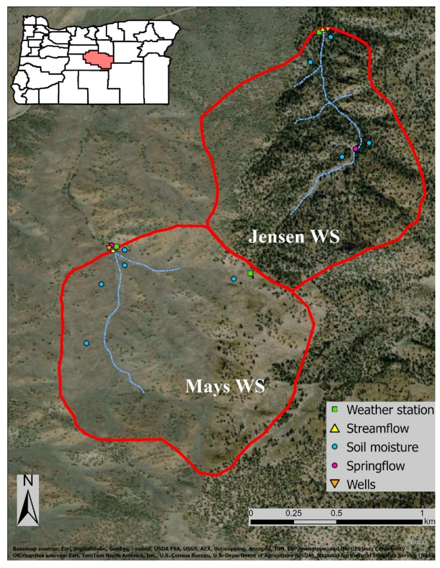
2.1. Site Description

This research was conducted at the Camp Creek Paired Watershed Study (CCPWS) site in central Oregon, USA. The CCPWS was established in 1993 to examine the potential impacts of juniper removal on hydrologic processes such as streamflow, soil water content, and groundwater. The CCPWS site includes two watersheds (WSs): Mays WS (116 hectares) and Jensen WS (96 hectares). The study site is located within the John Day ecological province [66]. Western juniper is the dominant overstory species at Jensen WS, while big sagebrush is the primary overstory species at Mays WS following juniper removal in 2005. Juniper canopy cover is 30% at the untreated Jensen WS and it is less than 1% at Mays WS [30,31,67]. Juniper density is 797 trees ha⁻¹ at Jensen WS, of which 21% (167 trees ha⁻¹) are estimated to be mature juniper, and 313 trees ha⁻¹ at Mays WS where most junipers are at the sapling stage [67]. The density of mature juniper at the Mays WS is 9.5 trees ha⁻¹ (unpublished data). Shrub cover, including big sagebrush and other species such as green rabbitbrush (Chrysothamnus viscidiflorus) and antelope bitterbrush (Purshia tridentata), is approximately 10% at the Jensen WS and 23% at the Mays WS [68]. At a study site approximately 9 km from CCPWS, Mollnau et al. [32] found that shrub density was approximately 2%. Similarly, Bates et al. [69] found that shrub cover was <1% at a study site in Southeastern Oregon, but this increased to 5.5% ± 1.3% 25 years after juniper removal. The CCPWS site consists of public and privately owned land and is largely used for cattle grazing. Most precipitation occurs as a mix of rain and snow during fall and winter. Long-term (1961–2016) average annual precipitation in the region is 322 mm, with daily snow depth reaching up to 480 mm [70].

Clarno and John Day formations dominate the geology in this region, with alluvium in the valleys. The low permeability of the deeper geologic strata has resulted in transient unconfined shallow aquifers that primarily follow surface topography and that are recharged during the winter precipitation and spring snowmelt runoff seasons [52]. The topography of Mays WS and Jensen WS are similar and are characterized by a relatively low gradient landscape. Elevation ranges from 1367 to 1524 m. The average slope is 24% for Mays WS and 25% for Jensen WS. The orientation of Mays WS is to the north–northwest, while Jensen WS is oriented to the north [71]. The soil series at CCPWS comprise Madeline Loam, Westbutte very stone loam, and Simas gravelly silt loam [71]. The Westbutte series covers approximately 50% of the area at Mays WS and 26% at Jensen WS. These soils are well-drained and moderately deep [71,72]. Soils in the Madeline loam series are shallow and well-drained and cover 20% of the area at Mays and 48% at Jensen [71,72]. The Simas soils are very deep and well-drained and cover 21% at Jensen WS and 3% at Mays WS [71,72].

In 2005 the CCPWS site was instrumented to measure multiple hydrologic (e.g., soil water content, groundwater, and streamflow) and weather parameters. Since 2014, additional monitoring locations and equipment have been included to measure other variables (e.g., springflow and tree transpiration) and expand the spatial understanding of ecohydrologic processes within and downstream of the treated (Mays WS) and untreated (Jensen WS) watersheds (Figure 1). Data collected between 2013 and 2020 were used to calculate the different water budget components described in this study.

2.2. Water Balance

A water-balance approach was used to calculate deep percolation (DP) below the top 0.8 m soil depth, which was assumed to be the effective rooting zone depth. This is based on observations made during soil-water-content sensor installation at multiple sites in the two watersheds, where it was noted that the soil’s profile was less than 1 m depth [30]. For each watershed, the quarterly portioning of different water budget components for each water year from 2014 to 2020 were obtained based on measurements of precipitation (P), soil volumetric water content (θ), streamflow (Q), and weather data used for modeling evapotranspiration (ET_A). These components were assumed to represent processes within the unsaturated soil zone. The following water-balance equation was used (Equation (1); all units are in mm day⁻¹).

$$DP=P-\mathsf{\Delta }\vartheta -Q-E{T}_A$$

(1)

The seasonal water budget of the unsaturated soil layer zone was calculated by summing the daily values for each component. This was performed for each quarter of the water year, with the first quarter corresponding to October through December. A seasonal water budget approach was selected to contrast periods of differing precipitation and temperature characteristics. The annual water budget based on the water year (1 October through 30 September) was calculated by summing the quarterly values for each water-balance component.

The seasonal patterns of precipitation were determined by using rain and snow data. Daily averaged levels of total P were calculated from data collected by using three tipping-bucket rain gauges installed onsite at each watershed outlet, and the watershed divide. Rain data near the outlet of each watershed was primarily used. However, during brief periods of data unavailability (e.g., equipment failures), precipitation records from the watershed divide (Figure 1) were used.

Snow-depth data were obtained by using an ultrasonic snow-depth-recording sensor (Model TS-15S, Automata, Inc., Nevada City, CA, USA) installed at the outlet of Mays WS. We characterized the annual snow-water equivalent (SWE) based on the snow-depth-sensor data and SWE: precipitation ratios derived from the nearest (Ochoco Meadows) SNOwpack TELemetry Network (SNOTEL) [73], located approximately 51 km north at an elevation of 1655 m. The ratio of the SNOTEL SWE to snowpack depth at this station was multiplied by the snowpack depth at CCPWS to estimate monthly SWE.

Daily changes in soil volumetric water content (∆θ) were obtained based on hourly records of θ from sensors installed at depths of 0.2, 0.5, and 0.8 m, as described in [30]. The Δθ was calculated for each soil depth, averaged across all three depths, and then divided by the total depth (0.8 m). The soil moisture stations used in this study are at locations representing different topographic and vegetation conditions within each watershed. At Jensen WS, soil moisture sensors are located in tree undercanopy and intercanopy sites at valley and upland sites. The stations at Mays WS, which is dominated by sagebrush, are likewise located in valley and upland sites (see [30]).

Streamflow (Q) was measured at the outlet of each watershed, using a type-H flume [74] equipped with a water-level logger (Model HOBO U20-001-01, Onset Computer, Corp.; Bourne, MA, USA). Water-stage data were collected every 15 min at the flume, and the manufacturer’s pre-calibrated equations were used to estimate Q.

The Hargreaves–Samani equation [41] was used to calculate potential evapotranspiration (PET) (Equation (2)) in mm day⁻¹. Mean (T_mean), maximum (T_max), and minimum (T_min) air temperature and solar radiation (R_a) data were collected onsite. All temperatures are in °C. Ra is in MJ m² day⁻¹. Additionally, a radiation adjustment coefficient (k_rs) of 0.17 was used based on Samani [75]. Due to the close proximity of the two watersheds and their relatively small size, it was assumed that ambient conditions (e.g., air temperature) and solar radiation would be similar, and therefore PET values would also be similar.

$$PET=0.0135\ast {\mathrm{k}}_{rs}\ast \left(T_{mean}+17.8\right)\ast {\left(T_{max}-T_{min}\right)}^{0.5}\ast 0.408\ast R_a$$

(2)

Daily estimates of ET_A were obtained by using a modified Thornthwaite-type water-balance equation, similar to that described by Alley [47] and Dingman [76] (Equations (3) and (4)). This approach was selected to reflect seasonal periods of energy-limited evapotranspiration (winter months) versus periods of water-limited evapotranspiration (generally late spring through fall).

$$\mathrm{When} PET>P-\mathsf{\Delta }\theta – Q, \mathrm{then} E{T}_A=P-\mathsf{\Delta }\theta – Q$$

(3)

$$\mathrm{When} PET \le P-\mathsf{\Delta }\theta – Q, \mathrm{then} E{T}_A=PET$$

(4)

2.3. Subsurface Flow and Shallow Aquifer Response to Seasonal Precipitation

Seasonal groundwater flow at each watershed was characterized by using data collected hourly with water-level loggers (Model HOBO U20-001-01, Onset Computer, Corp.; Bourne, MA, USA) installed in five (Mays WS) and six (Jensen WS) shallow groundwater-monitoring wells located near the outlet of each watershed (see Figure 1). The wells were located perpendicular to the stream channel and are numbered in order, generally from west to east (Mays WS wells, T1–T5; Jensen WS wells, U1–U6). The transect at Mays WS is 38 m across at an elevation of 1438 m and the transect at Jensen WS is 52 m across at an elevation of 1373 m. The Mays WS wells are primarily located in fractured rock substrate, while the Jensen WS wells are located in alluvium and fractured rock [68,77]. The maximum well depth was 8.2 m; however, some wells were somewhat shallower, with the bottom of all wells near or at the bedrock layer [30,77].

The recharge (Re_GW) of the shallow aquifer was estimated by using the WTFM [60]. The WTFM calculates recharge based on shallow, unconfined groundwater-level fluctuations and specific yield (S_y) [60], where S_y is multiplied by the change in water-table height (Δh) over time (Δt) (Equation (5)). Re was calculated at the daily time step (mm day⁻¹).

$$R{e}_{GW}=S_y\frac{\mathsf{\Delta }h}{\mathsf{\Delta }t}$$

(5)

The WTFM works best in shallow unconfined aquifers with sharp groundwater level rises and declines observed over short periods of time [60]. This is the case for the wells at our study site, where rapid changes in the water table are observed during the relatively short groundwater recharge season that peaks in early spring. Peak water level rises in the shallowest vs. the deepest wells ranged from 0.5 to 4.1 m at Mays WS and from 0.4 to 5.4 m at Jensen WS. For estimating groundwater recharge, the measurements of groundwater level, using a monitoring well, are believed to cover at least several tens of square meters [60]. Given that all monitoring wells used in this study are located within less than 50 m, in transects spanning across the entire valley bottom cross-section, we used data from two of the deepest wells in each transect (T3 at Mays WS and U5 at Jensen WS) to calculate aquifer recharge. The assumption was that these two wells would be representative of shallow groundwater dynamics occurring at the outlet of each watershed.

One of the challenges of using the WTFM is determining a representative value for S_y [56]. S_y indicates the volume of water drained out of the unconfined aquifer when the water table drops, and it is defined as the ratio of the volume of water that drains freely from a saturated substrate due to gravity forces to the total volume of the substrate [78]. To our knowledge, no shallow aquifer tests to determine S_y have been conducted in the region where our study site is located. Therefore, we used S_y values from the literature based on the medium gravel and tuff layers at Mays WS, and the fine-to-medium gravel at Jensen WS observed in the water-table-fluctuation zone during the installation of the wells (data not published). An average value of 0.23 for Mays WS and 0.26 for Jensen WS was obtained based on the S_y values for geological deposits reported by [76].

Springflow data were calculated based on a discharging spring in each watershed (Figure 1). The two relatively low flow springs have been re-conditioned to be able to measure springflow [30]. A springbox (0.6 m diameter by 1.8 m depth) to capture and discharge water to a cattle trough was installed at each site [77]. Springflow was measured regularly (bi-weekly to quarterly) from 2004 to 2020, except for 2014 and 2015, when no data were collected. Manual springflow measurements were made at the discharge pipe outlet, using a timer and a 5 L bucket. In 2017, a water level logger (Model HOBO U20-001-01, Onset Computer, Corp.; Bourne, MA, USA) was installed in each springbox to measure spring-water-level fluctuations hourly.

The upslope contributing area for the spring in Mays WS (112 ha) is greater than Jensen WS (51 ha). The Mays WS spring is located near the outlet of the WS, while the Jensen WS spring is located further upslope in the upper portion of the watershed. Based on the Jensen WS spring location, springflow is assumed to contribute to intermittent streamflow, soil water content, and shallow groundwater within the watershed. The springflow at Mays WS is assumed to reflect groundwater outflow from the watershed.

A stage–discharge curve was calculated based on the manual measurements of springflow and springbox water-level (stage). A high correlation (Pearson r = 0.95 for Mays WS and r = 0.95 for Jensen WS) was observed between springflow and spring water stage. A multilinear regression based on daily averaged θ in the contributing catchment was used to estimate daily springflow volume in the years before installing the water level loggers in each watershed’s springbox. Similar to the stage–discharge relationship, a relatively high correlation (r = 0.84 to 0.89 for Mays WS; r = 0.81 to 0.92 for Jensen WS) was observed between θ and springflow.

The Shapiro–Wilk test indicated that the springflow and groundwater-level data were not normally distributed; therefore, nonparametric statistical analyses were used. The Mann–Whitney Rank-Sum test was used to compare mean seasonal springflow rates between the two watersheds. The Kruskal–Wallis One-Way Analysis of Variance on Ranks (ANOVA) and Dunn’s Method were used to assess differences in groundwater level height for the 11 shallow groundwater wells. SigmaPlot^® version 14.0 (Systat Software, Inc., San Jose, CA, USA) was used for all the statistical analyses.

3. Results

3.1. Water Balance

The annual water-balance results by water year (October through September) for both watersheds are shown in

Table 1. Water-balance components by season and watershed. Each water year (October 31–September 30) is presented by quarter, with Q1 referring to October through December, etc.

		Mays WS					Jensen WS
Water Year	PET	P	Q	Δθ	ETA	DP	P	Q	Δθ	ETA	DP
2014 Q1	47.9	35.8	0.0	−29.3	47.9	17.2	26.1	0.0	−18.3	44.4	0.0
2014 Q2	46.2	111.5	0.4	63.1	46.2	1.8	100.8	0.0	56.6	44.2	0.0
2014 Q3	233.8	67.3	0.0	−27.8	95.1	0.0	60.2	0.0	−25.6	85.8	0.0
2014 Q4	287.3	51.3	0.4	−14.5	65.4	0.0	30.5	0.0	−10.3	40.8	0.0
2014 Total	615.2	265.9	0.8	−8.5	254.6	19.0	217.6	0.0	2.4	215.2	0.0
2015 Q1	46.6	169.9	0.0	36.8	46.6	86.5	165.6	0.0	53.2	46.6	65.8
2015 Q2	56.8	69.3	24.1	20.9	24.3	0.0	78.2	0.0	15.5	56.8	5.9
2015 Q3	224.9	59.4	0.0	−31.3	90.7	0.0	54.6	0.0	−40.0	94.6	0.0
2015 Q4	286.6	42.9	0.0	−27.0	69.9	0.0	44.7	0.0	−27.5	72.2	0.0
2015 Total	614.9	341.6	24.1	−0.6	231.6	86.5	343.2	0.0	1.2	270.2	71.7
2016 Q1	44.2	129.3	0.0	25.7	44.2	78.2	111.5	0.0	42.1	44.2	25.2
2016 Q2	41.8	97.8	19.9	35.2	41.8	0.9	111.3	0.0	32.8	41.8	36.6
2016 Q3	232.4	69.3	4.1	−11.4	121.9	0.0	64.5	0.0	−29.4	93.9	0.0
2016 Q4	305.8	1.8	0.0	−42.5	44.3	0.0	12.2	0.0	−43.1	55.3	0.0
2016 Total	624.3	298.2	24.0	7.0	252.1	79.1	299.5	0.0	2.4	235.2	61.8
2017 Q1	44.0	116.6	0.0	−2.1	44.0	74.7	125.5	0.0	5.8	44.0	75.7
2017 Q2	37.6	169.1	26.1	86.1	37.6	45.8	156.0	1.5	88.6	37.6	28.3
2017 Q3	220.2	75.4	35.3	−43.7	83.8	0.0	73.9	2.1	−48.4	120.2	0.0
2017 Q4	332.4	15.0	0.8	−30.5	44.7	0.0	14.0	0.1	−32.8	46.7	0.0
2017 Total	634.1	376.1	62.2	9.8	210.1	120.5	369.3	3.7	13.2	248.5	103.9
2018 Q1	52.4	55.0	0.0	−10.0	52.4	12.6	68.4	0.0	−9.4	52.4	25.4
2018 Q2	43.6	61.0	0.0	51.4	9.6	0.0	72.9	0.0	49.7	23.2	0.0
2018 Q3	223.1	82.8	0.0	−26.4	109.2	0.0	80.1	0.5	−20.1	99.7	0.0
2018 Q4	364.0	27.5	0.0	−31.6	59.1	0.0	4.1	0.1	−21.5	25.5	0.0
2018 Total	683.0	226.3	0.0	−16.6	230.3	12.6	225.5	0.6	−1.3	200.7	25.4
2019 Q1	54.2	74.7	0.0	15.4	54.2	5.1	80.3	0.0	−1.1	54.2	27.2
2019 Q2	50.0	108.0	1.0	94.1	12.9	0.0	101.7	2.4	70.3	29.0	0.0
2019 Q3	207.9	83.2	26.7	−45.0	101.5	0.0	77.8	1.1	−29.2	105.9	0.0
2019 Q4	288.3	60.3	0.0	−30.9	91.2	0.0	71.6	0.0	−28.0	99.6	0.0
2019 Total	600.4	326.1	27.7	33.6	259.8	5.1	331.4	3.5	12.0	288.8	27.2
2020 Q1	45.6	87.6	0.0	17.4	45.6	24.7	70.1	0.0	11.5	45.6	12.9
2020 Q2	46.0	88.3	0.0	61.9	26.4	0.0	73.5	0.0	31.6	41.9	0.0
2020 Q3	187.9	81.0	0.0	−68.7	149.7	0.0	66.0	0.0	−38.7	104.7	0.0
2020 Q4	306.8	9.0	0.0	−25.7	34.7	0.0	8.3	0.0	−16.2	24.5	0.0
2020 Total	586.3	265.9	0.0	−15.2	256.4	24.7	217.8	0.0	−11.8	216.7	12.9

. ET_A accounted for the largest portion of the annual water budget within both watersheds, averaging 83% of incoming precipitation at Mays WS and 86% of incoming precipitation at Jensen WS. At Mays WS, ET_A ranged from 210 to 260 mm yr⁻¹ (mean of 242 mm yr⁻¹). The ET_A at Jensen WS ranged from 201 to 289 mm yr⁻¹ (mean of 239 mm yr⁻¹). DP ranged from 5 to 121 mm yr⁻¹ (mean of 50 mm yr⁻¹) at Mays WS and from 0 to 104 mm yr⁻¹ (mean of 43 mm yr⁻¹) at Jensen WS.

Using data collected and described by Abdallah et al. [33] and density estimates from Durfee et al. [67], we estimated that transpiration associated with mature juniper at Jensen WS to be between 0.35 and 1.9 mm day⁻¹ and between 0.03 and 0.16 mm day⁻¹ at Mays WS for the time periods observed. The greater transpiration rate associated with juniper at Jensen WS is associated with the greater density of mature juniper in that WS. For saplings, estimated transpiration ranged from 0.01 to 0.09 mm day⁻¹ at Mays WS and 0.01 to 0.18 mm day⁻¹ at Jensen WS. Transpiration estimates were not available for the whole year, and therefore we did not calculate yearly juniper transpiration rates as a portion of the water budget.

Peaks in seasonal ET_A occurred during Q3 (April through June), which corresponds to periods of snowmelt. The average ET_A during Q3 was 107 mm at Mays WS and 101 mm at Jensen WS. Seasonal ET_A was generally lowest during Q2 (January through March), corresponding to periods of lowest temperatures and highest snowmelt. Mean ET_A at Mays WS was 28 mm and at Jensen WS was 39 mm during the second quarter.

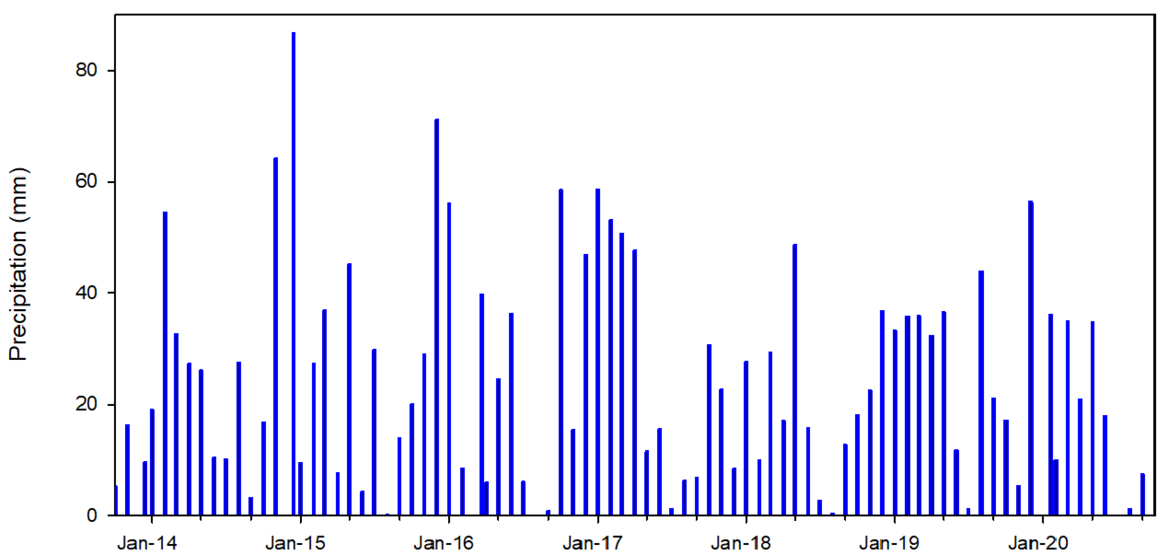
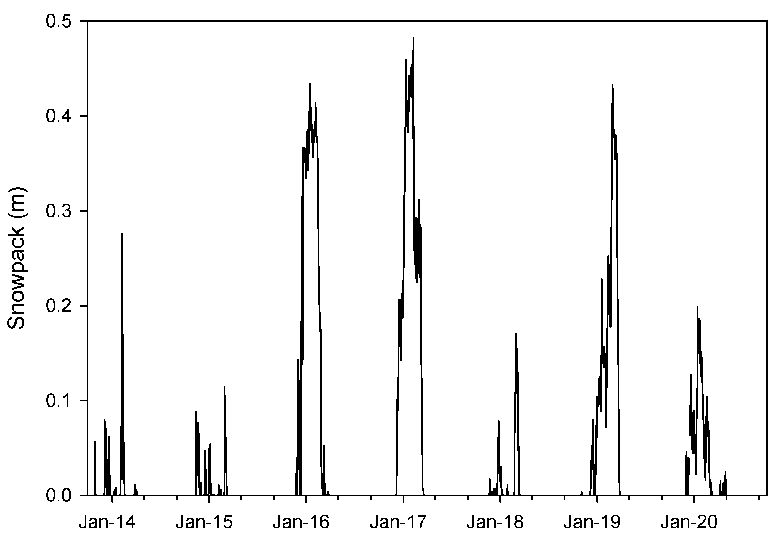
3.1.1. Snowpack and Precipitation Patterns

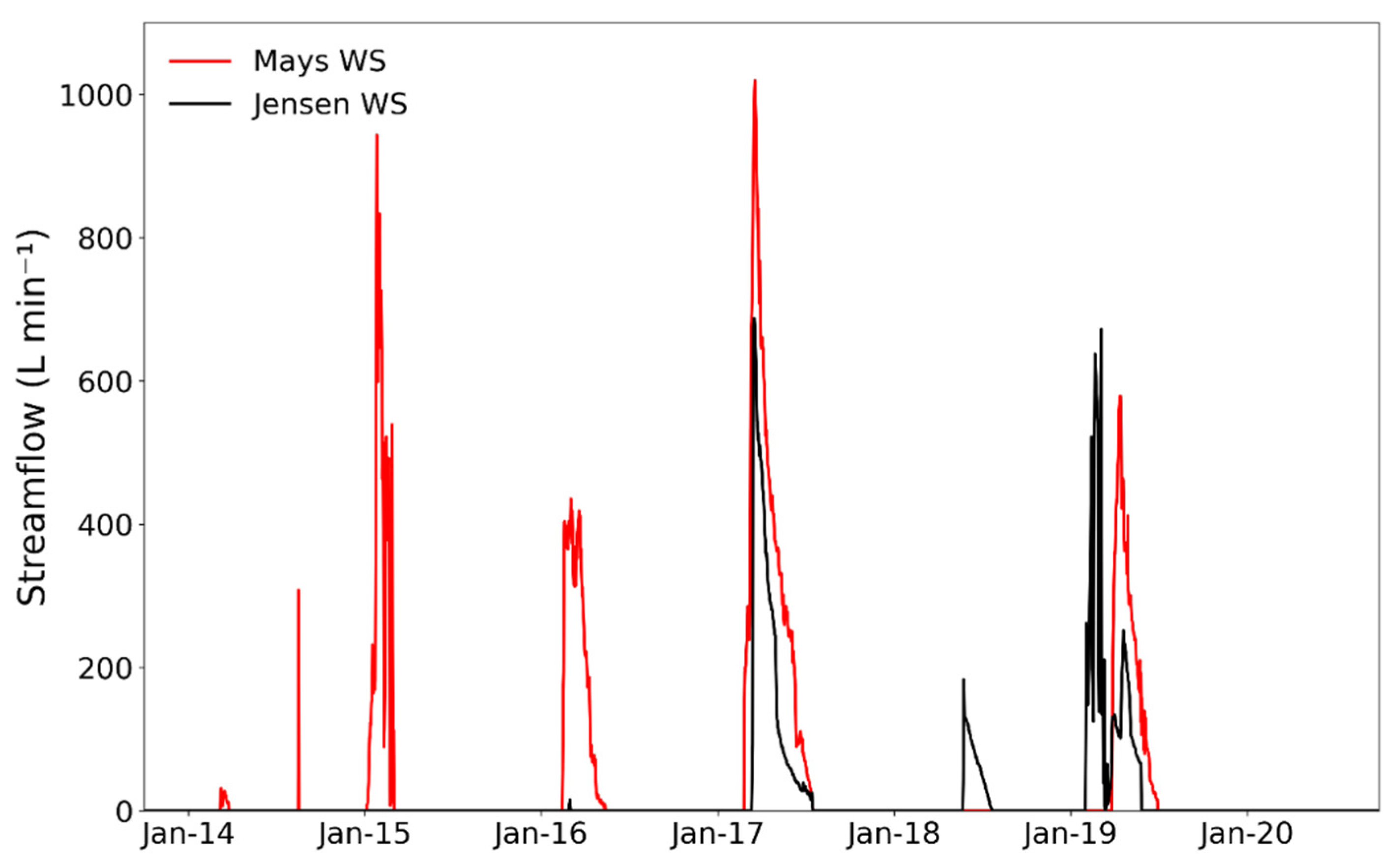
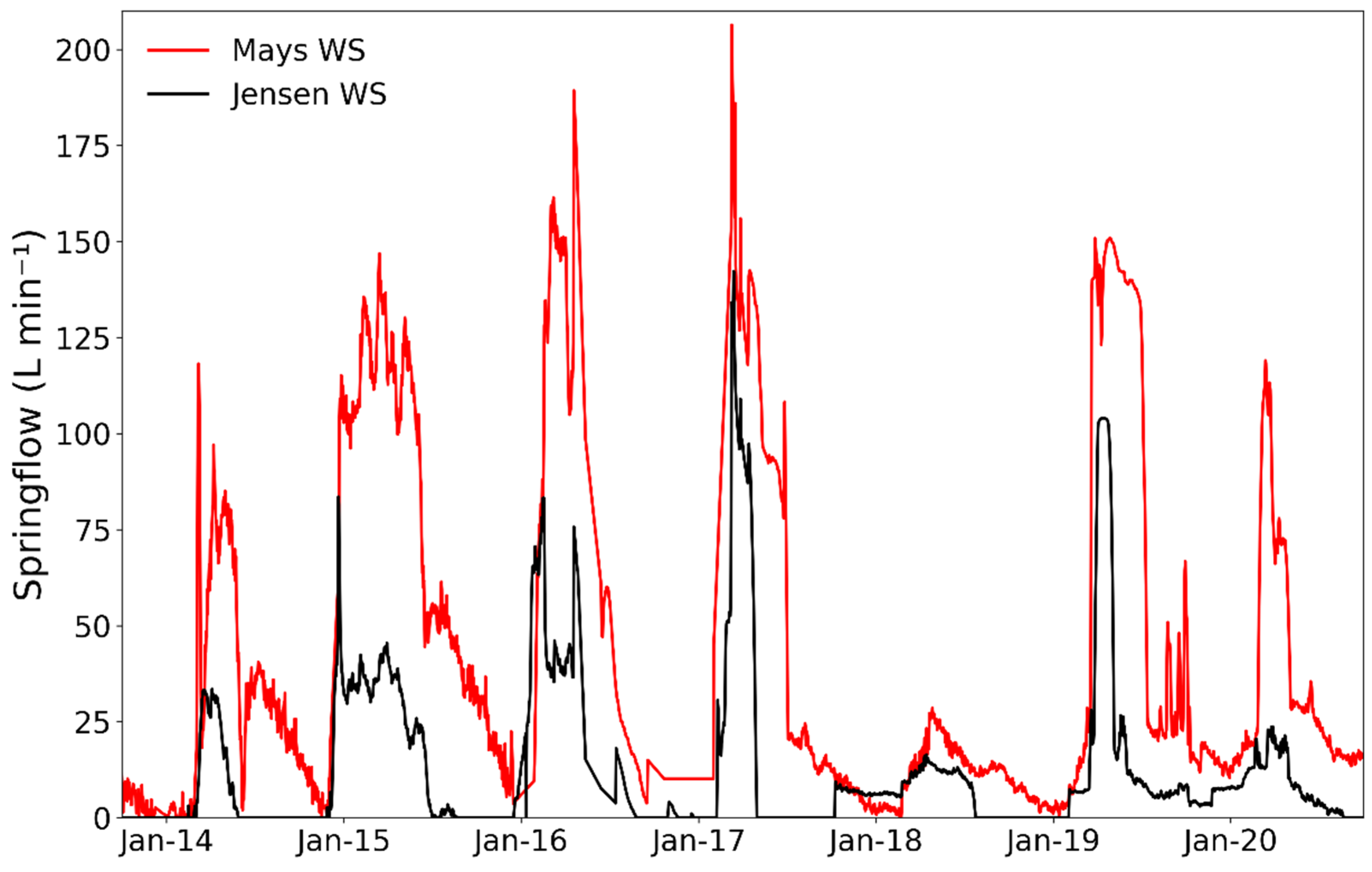
Annual precipitation was similar in the two watersheds. The average precipitation between the two watersheds was 293 mm yr⁻¹; ranging from 218 to 376 mm (Figure 2). Precipitation primarily fell during Q2 (January through March) (Figure 2), when ET is energy-limited. However, considerable variation was seen in seasonal precipitation patterns over the course of this study (see Table 1), even during years with similar amounts of total annual precipitation.

In general, snow accumulated from November to January of each year, with Figure 3. Annual variations in both snowfall and depth were observed across years during this study. Snowpack levels and SWE varied from year to year, even between years with similar total annual precipitation (e.g., 2014 and 2018). The 2017 water year showed the greatest SWE while the 2018 water year showed the least. SWE generally peaked in January (mean SWE of 40 mm) or February (mean SWE of 43 mm). Reflecting snowpack, SWE varied from 0.2 to 106 mm in January and from 3 to 100 mm in February. Mean December SWE was 25 mm, ranging from 3 to 74 mm. Mean March SWE was 17 mm, ranging from 0.2 to 69 mm.

3.1.2. Streamflow

On average, streamflow at Mays WS accounted for 5.8% of incoming precipitation, ranging from 0% to 17% for individual water years. At Jensen WS, streamflow accounted for an average of 0.3% of incoming precipitation, ranging from 0% to 1.1%.

In general, seasons of greatest streamflow corresponded to snowmelt and increased soil water content periods in March and April. In most years, streamflow peaked in Q2 (January through March) or Q3, generally corresponding to snowmelt. However, smaller streamflow amounts also periodically occurred in response to warmer season rainfall.

Years with the highest precipitation experienced the highest volume of streamflow (Figure 4). The timing of peak streamflow was similar in both watersheds, except for the 2019 water year, in which peak flow occurred at the Jensen WS several weeks sooner than it did at the Mays WS. In 2020, no streamflow was recorded at either WS; however, limited pooling was noted in the stream channel at both watersheds. Occasional convective summer storms resulted in streamflow during the summer months. During some of the larger summer storms, sediment accumulation in the flumes prevented accurate measurements of streamflow.

3.1.3. Soil-Water-Content Change

The soil-water-content change (∆θ) accounted for between −7.3% and 10.3% of the annual water budget at Mays WS and −5.4% and 3.6% at Jensen WS. Across all water years, the average ∆θ accounted for −0.2% of the annual water budget at Mays WS and 0.5% at Jensen WS.

While ∆θ accounted for a small portion of the annual water budget (on average, 1 mm at Mays WS and 3 mm at Jensen WS), it did show large shifts from season to season (see Table 1). Seasonal ∆θ ranged from −69 to 94 mm at Mays WS and from −48 to 89 mm at Jensen WS. In general, increased ∆θ occurred during Q2 (mean of 59 mm at Mays WS and 49 mm at Jensen WS), and decreased ∆θ occurred in Q3 (mean of −36 mm at Mays WS and −33 mm at Jensen WS) and Q4 (mean of −29 mm at Mays WS and −26 mm at Jensen WS).

3.1.4. Seasonal PET

The mean annual PET was 623 mm yr⁻¹ and ranged from 586 to 683 mm yr⁻¹. PET was on average 2.2 times greater than P on an annual basis. The balance of the water budget exceeded PET during Q1 for most years (see Table 1), which corresponds to the periods when increases in groundwater levels occurred. Given that the watersheds are adjacent to each other and experience similar temperature regimes and solar radiation, we assumed that PET was the same at both watersheds.

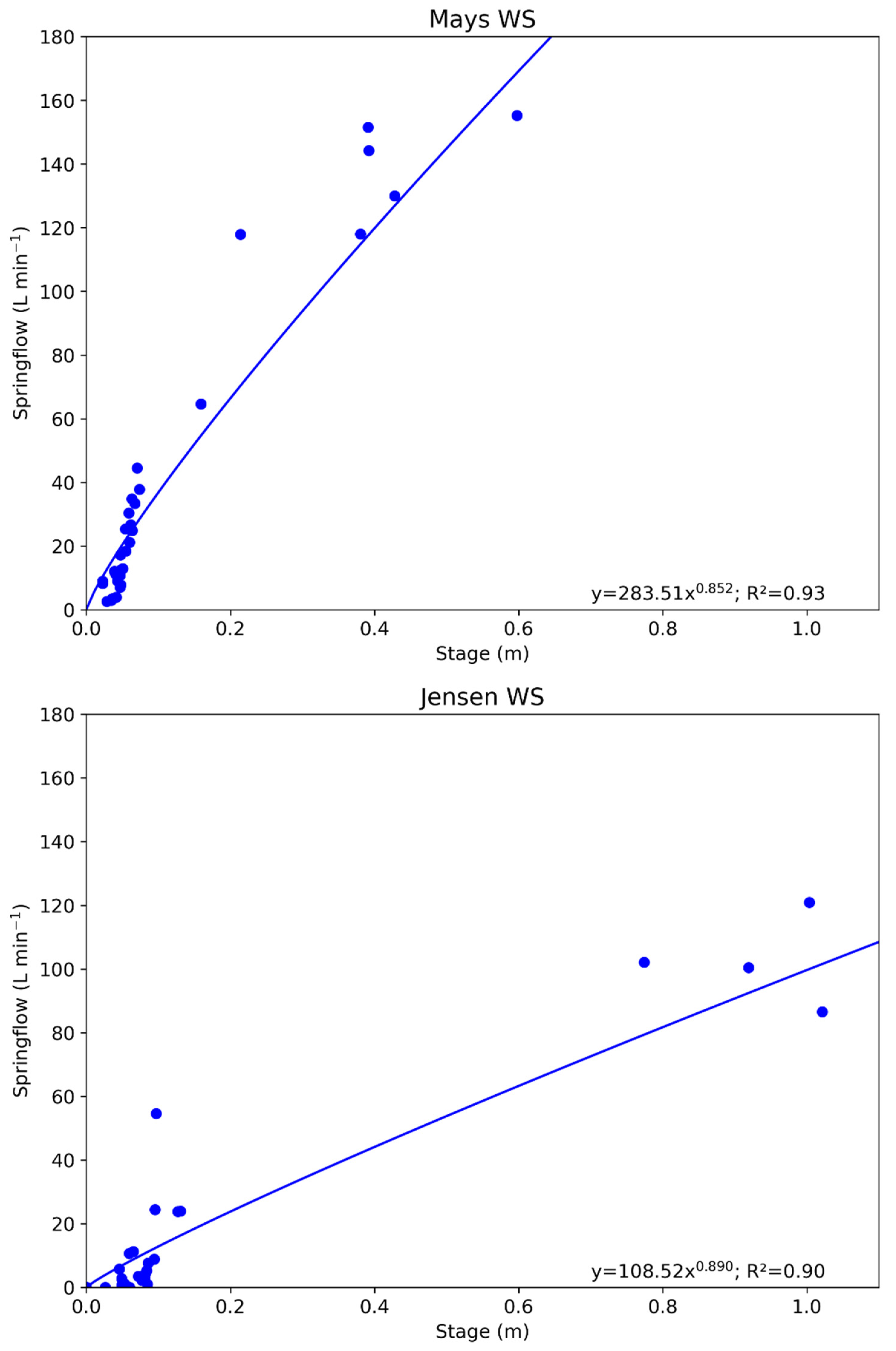
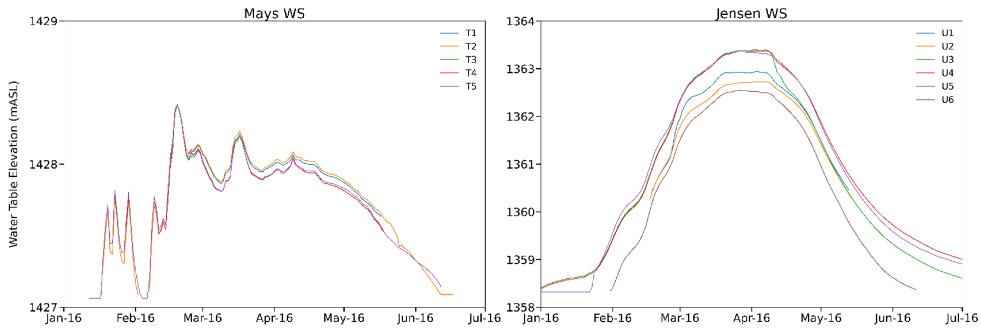
3.2. Subsurface Flow and Shallow Aquifer Response to Seasonal Precipitation

Similar to streamflow levels, the highest springflow rates obtained corresponded to periods of snowmelt in the spring and increased soil water content that typically occurred in winter and spring. Years with the highest precipitation generally experienced higher springflow rates, which peaked in Q3 (April through June) for most water years (Figure 5). Springflow rates were generally higher at Mays WS compared to Jensen WS. The mean springflow rate at Mays WS was 43.4 L min⁻¹, and it was 12.6 L min⁻¹ at Jensen WS. The Mann–Whitney Rank Sum test indicated a statistically significant difference (p ≤ 0.001, U = 13,748) in median daily springflow rates between the two watersheds (5.4 L min⁻¹ at Jensen WS vs. 20.6 L min⁻¹ at Mays WS).

Manual measurements of springflow and water level records from the springbox were used to create a stage–discharge curve (Figure 6). The majority of observed springflow rates were less than 50 L min⁻¹, with spring well-water levels less than 0.1 m at Mays WS and 0.2 m at Jensen WS.

Shallow groundwater level fluctuations showed a seasonal response to winter precipitation and snowmelt. All wells in each transect showed similar responses every year, as illustrated in Figure 7 for 2016. A pattern of less pronounced but more frequent groundwater level rises and declines was observed in the fractured basalt-dominated aquifer at Mays WS. A pattern of more pronounced and steadier groundwater level rises and declines was observed in the alluvium-dominated aquifer at Jensen WS. Peak groundwater levels at Mays WS were generally observed in February or March, while peak groundwater levels at Jensen were observed in late March or April every year (Figure 7).

The annual recharge of the shallow aquifer was highly variable in each watershed during the seven years evaluated (

Table 2. Annual groundwater recharge (Re_GW) and total precipitation (P) in the sagebrush-dominated watershed (Mays WS) and the juniper-dominated watershed (Jennsen WS). All measurements are in mm.

	Mays WS		Jensen WS
Water Year	ReGW	P	ReGW	P
2014	276	266	219	218
2015	862	342	659	343
2016	862	298	1311	300
2017	1263	376	1441	369
2018	0	226	35	226
2019	1371	326	1360	331
2020	318	266	632	218

). Annual Re_GW ranged from 0 to 1371 mm in Mays WS (mean of 707 mm) and from 35 to 1441 mm in Jensen WS (mean of 808 mm). The ANOVA results showed mean annual Re_GW was not significantly different (p > 0.05) between the two watersheds. In general, the highest Re_GW values were obtained during the years with the greatest snowpack depths (see Figure 3).

4. Discussion

This research examined the seasonal variability of various water budget components (e.g., evapotranspiration, precipitation, and deep percolation) and shallow aquifer recharge in cool-climate rangeland ecosystems in a semiarid region in central Oregon, USA. Specifically, we sought to (1) determine the partitioning of several water budget components in a western-juniper-dominated watershed and a sagebrush-dominated watershed; and (2) characterize shallow groundwater-level fluctuations in response to seasonal precipitation.

Similar to other studies [79,80,81,82], this research highlights the importance of seasonal precipitation patterns in semiarid environments in driving the response of many water budget components and the replenishment of the local aquifer. Study results show that evapotranspiration (ET) accounted for 83% of total annual precipitation in the sagebrush-dominated watershed (Mays WS) and 86% in the juniper-dominated watershed (Jensen WS). This is similar to that reported for other snow-dominated rangelands in the region. For a study site in Southwestern Idaho, USA, Kormos et al. [10] modeled the ET of a juniper-dominated site to be 80% of incoming precipitation and ET at a sagebrush-dominated site to be 61% of incoming precipitation. Flerchinger and Cooley [55] found that ET accounted for 90% of annual precipitation for a semiarid subbasin in Southwestern ID, USA.

Limited research has been conducted into the ET of western juniper and sagebrush steppe ecosystems. Studies have largely focused on transpiration, particularly of western juniper. Mollnau et al. [32] found that mature western juniper stand transpiration rates at a site in Central Oregon were approximately 0.4 mm per day during summer months and that transpiration rates were largely associated with soil water content. Abdallah et al. [33] found that peak transpiration rates of western juniper trees ranged from 73 to 115 L day⁻¹, varying with seasonal and annual precipitation and soil water content. Calculations of sagebrush transpiration are very limited. Valayamkunnath et al. [37] estimated sagebrush transpiration to be between 229 and 353 mm yr⁻¹, or 91–98% of the annual water budget, at a study site in Idaho.

Among the limitations of this study, the water balance method (WBM) approach applied cannot distinguish between precipitation that evaporates from juniper overstory, soil evaporation, or transpiration. As mature western juniper intercepts as much as 46% of precipitation at Jensen WS [30], there may be important differences in evaporation and transpiration rates not reflected by the WBM approach. Further, the WBM does not account for spatial variability (e.g., snowdrift, topographic variations in precipitation, or variations in vegetation cover) or connections between hydrologic processes (e.g., transmission losses in the stream channel and subsurface flow). It should be noted that for our study, streamflow measurements do not reflect potential stream channel transmission losses that may have occurred upslope of the flume at the outlet of the watershed.

Seasonal soil water storage is critical in sagebrush ecosystems [6]. Reduced soil water content has been associated with reduced net ecosystem exchange in sagebrush ecosystems in Wyoming [83]. In our study, the soil water content increased during the coldest and wettest months (January through March) at both watersheds and subsequently decreased in the following months. These seasonal increases corresponded to periods of highest annual precipitation and low PET. Additionally, we calculated daily soil-water-content change for a soil depth of 0.8 m, which we assumed represented the maximum rooting and soil depth for most of the two watersheds. This based on our observations of soil depth during sensor installation and the results of other studies [84,85]. However, the maximum rooting depth within each watershed may have varied due to specific site characteristics, including vegetation density and soil depth.

Winter precipitation and snowmelt runoff in the spring were reflected in the greater soil moisture and subsurface flows observed in both watersheds. Deep percolation (DP) below the root zone, calculated by using the WBM, and shallow aquifer recharge (Re_GW), estimated by using the WTFM, occurred during the wet season (winter–spring). Re_GW rates tended to decrease as juniper transpiration increased (based on data described by Abdallah et al. [33]); however, some interannual variability was shown. Seasonal variations in precipitation resulted in variations in DP and Re_GW, even during years when total precipitation amounts are similar. This was particularly the case in years when precipitation type was different (rain vs. snow). The WBM used in this study calculates DP as the sink term but does not account for incoming precipitation that may percolate through fractures in the soil or for differences in rain vs. snow, and therefore may underestimate the amount of DP. A significant portion of the DP estimated was expected to reach the shallow aquifer in each watershed; however, it is difficult to equate to Re_GW given some DP can move laterally out of the watershed or through the spring system. As discussed in [51], fractured basalt substrates, like the one found at our study site, may not necessarily lead to recharge but could also result in lateral flows.

A key premise of WTFM is that the specific yield (S_y) is constant over a given area and timeframe. If these assumptions are not met, then the groundwater recharge calculations may not be accurate for a given area. The WTFM assumes that increases in shallow groundwater heights are associated with aquifer recharge, although other processes, such as evapotranspiration, can also result in shallow groundwater fluctuations [60]. In particular, assumptions regarding the baseline recession (the decrease in groundwater levels that would have occurred with no recharge) will influence recharge calculations. Similar to methods used by [61,86,87], we assumed daily increases in groundwater level would reflect recharge rates. While this approach has been found to underestimate recharge compared to other WTFM approaches [88], we used frequent measurements (recorded hourly for the majority of the study and averaged at the daily time step) to minimize these discrepancies.

The decline in groundwater levels, consequently less Re_GW, observed during late spring was attributed to a combination of less snowmelt runoff inputs and the increased vegetation water uptake during the warmer spring days. Annual Re_GW was, for most years, several times that of the total precipitation for the water year, indicating spatial heterogeneity in recharge rates. We attributed this Re_GW response to the wells’ location at the watershed outlet, which may have accounted for the aggregate of subsurface flow coming out of the watersheds. However, it is difficult to extrapolate the results observed at the drainage outlet to the entire watershed, particularly with the varying topography, vegetation, and subsurface characteristics found at our study site.

In years with greater snowpack, streamflow and springflow levels were generally higher compared to rain-dominated years, even when annual precipitation amounts were nearly the same. As in Kormos et al. [10], significantly higher streamflow rates were observed in the sagebrush-dominated watershed. This was the case in the two years (2016 and 2017) with greater snowpack depths. Also, higher springflow rates were obtained in the sagebrush-dominated watershed for all years evaluated. This was partly attributed to the greater subsurface flow residence time observed in the sagebrush-dominated watershed, as previously documented in [30]. While springflow has been relatively the same at the juniper-dominated watershed, springflow in the sagebrush-dominated watershed is twice that found before juniper removal in 2005 [30]. The smaller catchment area draining into the spring in the juniper-dominated watershed may have also contributed to the lower springflow rates observed. Streamflow and springflow accounted for a relatively small portion of incoming precipitation, yet, both play an important role in the ecohydrology of the site. For instance, springflow is an important water source for cattle and wildlife for most of the year. Also, transient streamflow and subsurface flow help maintain the hydrologic connectivity between the upland watersheds and the larger valley they drain into [30].

While additional research is needed into quantifying recharge and evapotranspiration rates, particularly across a heterogeneous landscape, the results of this study contribute to the understanding of how woody plant encroachment and climate variability collectively affect the water budget in sagebrush and western juniper ecosystems. Combining ground-based techniques and remote sensing can improve our understanding of the spatial and temporal patterns of vegetation and soil water content in these watersheds. Future research at this site includes the continued monitoring of ecohydrologic characteristics and modeling applications to expand local results to larger spatial domains.

5. Conclusions

This study examined seasonal water balance and subsurface flow dynamics in two rangeland watersheds, one dominated by western juniper and one dominated by big sagebrush, in central Oregon, USA. We assessed seven years of observations with varied meteorological conditions. A water-balance-method approach was used to quantify multiple components of the water budget in each watershed. The Water-Table-Fluctuation-Method was used to calculate shallow aquifer recharge at the outlet of each watershed. Evapotranspiration accounted for most of the water budget, followed by deep percolation. Overall, greater springflow and streamflow rates were observed in the sagebrush-dominated watershed. There were no statistically significant differences in groundwater recharge rates between the juniper-dominated site overlying alluvium substrate and the sagebrush-dominated site overlying fractured basalt. However, the significant springflow levels observed at the outlet of the sagebrush-dominated basin added to the total amount of subsurface flow coming out of the watershed. Aquifer recharge and springflow estimates were higher in both watersheds during the years with less potential evapotranspiration and greater snowpack. This study provides important information regarding the seasonal precipitation dynamics affecting the portioning of different water-budget components and the mechanisms of shallow aquifer replenishment in juniper- vs. sagebrush-dominated landscapes. Further research is needed to expand on the temporal and spatial dynamics of the ecohydrologic processes and land-management practices affecting water availability in cool-climate rangeland ecosystems.

References

1. Bradford, J.B.; Schlaepfer, D.R.; Lauenroth, W.K. Ecohydrology of Adjacent Sagebrush and Lodgepole Pine Ecosystems: The Consequences of Climate Change and Disturbance. Ecosystems 2014, 17, 590–605. [Google Scholar] [CrossRef]
2. Palmquist, K.A.; Schlaepfer, D.R.; Bradford, J.B.; Lauenroth, W.K. Mid-Latitude Shrub Steppe Plant Communities: Climate Change Consequences for Soil Water Resources. Ecology 2016, 97, 2342–2354. [Google Scholar] [CrossRef] [PubMed]
3. Abdulla, F.; Eshtawi, T.; Assaf, H. Assessment of the Impact of Potential Climate Change on the Water Balance of a Semi-Arid Watershed. Water Resour. Manag. 2009, 23, 2051–2068. [Google Scholar] [CrossRef]
4. Eckhardt, K.; Ulbrich, U. Potential Impacts of Climate Change on Groundwater Recharge and Streamflow in a Central European Low Mountain Range. J. Hydrol. 2003, 284, 244–252. [Google Scholar] [CrossRef]
5. Meixner, T.; Manning, A.H.; Stonestrom, D.A.; Allen, D.M.; Ajami, H.; Blasch, K.W.; Brookfield, A.E.; Castro, C.L.; Clark, J.F.; Gochis, D.J.; et al. Implications of Projected Climate Change for Groundwater Recharge in the Western United States. J. Hydrol. 2016, 534, 124–138. [Google Scholar] [CrossRef] [Green Version]
6. Schlaepfer, D.R.; Lauenroth, W.K.; Bradford, J.B. Consequences of Declining Snow Accumulation for Water Balance of Mid-Latitude Dry Regions. Glob. Chang. Biol. 2012, 18, 1988–1997. [Google Scholar] [CrossRef]
7. Konapala, G.; Mishra, A.K.; Wada, Y.; Mann, M.E. Climate Change Will Affect Global Water Availability through Compounding Changes in Seasonal Precipitation and Evaporation. Nat. Commun. 2020, 11, 3044. [Google Scholar] [CrossRef]
8. Bradford, J.B.; Schlaepfer, D.R.; Lauenroth, W.K.; Burke, I.C. Shifts in Plant Functional Types Have Time-Dependent and Regionally Variable Impacts on Dryland Ecosystem Water Balance. J. Ecol. 2014, 102, 1408–1418. [Google Scholar] [CrossRef]
9. Pierson, F.B.; Jason Williams, C.; Hardegree, S.P.; Clark, P.E.; Kormos, P.R.; Al-Hamdan, O.Z. Hydrologic and Erosion Responses of Sagebrush Steppe Following Juniper Encroachment, Wildfire, and Tree Cutting. Rangel. Ecol. Manag. 2013, 66, 274–289. [Google Scholar] [CrossRef] [Green Version]
10. Kormos, P.R.; Marks, D.; Pierson, F.B.; Williams, C.J.; Hardegree, S.P.; Havens, S.; Hedrick, A.; Bates, J.D.; Svejcar, T.J. Ecosystem Water Availability in Juniper versus Sagebrush Snow-Dominated Rangelands. Rangel. Ecol. Manag. 2017, 70, 116–128. [Google Scholar] [CrossRef] [Green Version]
11. Petersen, S.L.; Stringham, T.K. Infiltration, Runoff, and Sediment Yield in Response to Western Juniper Encroachment in Southeast Oregon. Rangel. Ecol. Manag. 2008, 61, 74–81. [Google Scholar] [CrossRef]
12. Bradley, B.A. Assessing Ecosystem Threats from Global and Regional Change: Hierarchical Modeling of Risk to Sagebrush Ecosystems from Climate Change, Land Use and Invasive Species in Nevada, USA. Ecography 2010, 33, 198–208. [Google Scholar] [CrossRef]
13. Creutzburg, M.K.; Halofsky, J.E.; Halofsky, J.S.; Christopher, T.A. Climate Change and Land Management in the Rangelands of Central Oregon. Environ. Manag. 2015, 55, 43–55. [Google Scholar] [CrossRef] [PubMed]
14. Valayamkunnath, P.; Sridhar, V.; Zhao, W.; Allen, R.G. A Comprehensive Analysis of Interseasonal and Interannual Energy and Water Balance Dynamics in Semiarid Shrubland and Forest Ecosystems. Sci. Total Environ. 2019, 651, 381–398. [Google Scholar] [CrossRef] [PubMed]
15. Scott, R.L.; Biederman, J.A. Critical Zone Water Balance Over 13 Years in a Semiarid Savanna. Water Resour. Res. 2019, 55, 574–588. [Google Scholar] [CrossRef] [Green Version]
16. Lewis, D.; Singer, M.J.; Dahlgren, R.A.; Tate, K.W. Hydrology in a California Oak Woodland Watershed: A 17-Year Study. J. Hydrol. 2000, 240, 106–117. [Google Scholar] [CrossRef]
17. Yang, Y.; Liu, D.L.; Anwar, M.R.; O’Leary, G.; Macadam, I.; Yang, Y. Water Use Efficiency and Crop Water Balance of Rainfed Wheat in a Semi-Arid Environment: Sensitivity of Future Changes to Projected Climate Changes and Soil Type. Theor. Appl. Climatol. 2016, 123, 565–580. [Google Scholar] [CrossRef]
18. Kundu, S.; Khare, D.; Mondal, A. Past, Present and Future Land Use Changes and Their Impact on Water Balance. J. Environ. Manag. 2017, 197, 582–596. [Google Scholar] [CrossRef]
19. Chauvin, G.M.; Flerchinger, G.N.; Link, T.E.; Marks, D.; Winstral, A.H.; Seyfried, M.S. Long-Term Water Balance and Conceptual Model of a Semi-Arid Mountainous Catchment. J. Hydrol. 2011, 400, 133–143. [Google Scholar] [CrossRef] [Green Version]
20. Marc, V.; Robinson, M. The Long-Term Water Balance (1972–2004) of Upland Forestry and Grassland at Plynlimon, Mid-Wales. Hydrol. Earth Syst. Sci. 2007, 11, 44–60. [Google Scholar] [CrossRef] [Green Version]
21. Ward, A.S.; Gooseff, M.N.; Voltz, T.J.; Fitzgerald, M.; Singha, K.; Zarnetske, J.P. How Does Rapidly Changing Discharge during Storm Events Affect Transient Storage and Channel Water Balance in a Headwater Mountain Stream? Water Resour. Res. 2013, 49, 5473–5486. [Google Scholar] [CrossRef]
22. Wang, D.; Alimohammadi, N. Responses of Annual Runoff, Evaporation, and Storage Change to Climate Variability at the Watershed Scale. Water Resour. Res. 2012, 48. [Google Scholar] [CrossRef] [Green Version]
23. do Nascimento, M.G.; Herdies, D.L.; de Souza, D.O. The South American Water Balance: The Influence of Low-Level Jets. J. Clim. 2016, 29, 1429–1449. [Google Scholar] [CrossRef]
24. Weltz, M.A.; Blackburn, W.H. Water Budget for South Texas Rangelands. J. Range Manag. 1995, 48, 45–52. [Google Scholar] [CrossRef]
25. Wilcox, B.P.; Dowhower, S.L.; Teague, W.R.; Thurow, T.L. Long-Term Water Balance in a Semiarid Shrubland. Rangel. Ecol. Manag. 2006, 59, 600–606. [Google Scholar] [CrossRef]
26. Bugan, R.; Jovanovic, N.; De Clercq, W. The Water Balance of a Seasonal Stream in the Semi-Arid Western Cape (South Africa). WSA 2012, 38, 201–212. [Google Scholar] [CrossRef] [Green Version]
27. Cantón, Y.; Villagarcía, L.; Moro, M.J.; Serrano-Ortíz, P.; Were, A.; Alcalá, F.J.; Kowalski, A.S.; Solé-Benet, A.; Lázaro, R.; Domingo, F. Temporal Dynamics of Soil Water Balance Components in a Karst Range in Southeastern Spain: Estimation of Potential Recharge. Hydrol. Sci. J. 2010, 55, 737–753. [Google Scholar] [CrossRef] [Green Version]
28. Deus, D.; Gloaguen, R.; Krause, P. Water Balance Modeling in a Semi-Arid Environment with Limited in Situ Data Using Remote Sensing in Lake Manyara, East African Rift, Tanzania. Remote Sens. 2013, 5, 1651–1680. [Google Scholar] [CrossRef] [Green Version]
29. Eilers, V.H.M.; Carter, R.C.; Rushton, K.R. A Single Layer Soil Water Balance Model for Estimating Deep Drainage (Potential Recharge): An Application to Cropped Land in Semi-Arid North-East Nigeria. Geoderma 2007, 140, 119–131. [Google Scholar] [CrossRef] [Green Version]
30. Ochoa, C.; Caruso, P.; Ray, G.; Deboodt, T.; Jarvis, W.; Guldan, S. Ecohydrologic Connections in Semiarid Watershed Systems of Central Oregon USA. Water 2018, 10, 181. [Google Scholar] [CrossRef] [Green Version]
31. Ray, G.; Ochoa, C.G.; Deboodt, T.; Mata-Gonzalez, R. Overstory–Understory Vegetation Cover and Soil Water Content Observations in Western Juniper Woodlands: A Paired Watershed Study in Central Oregon, USA. Forests 2019, 10, 151. [Google Scholar] [CrossRef] [Green Version]
32. Mollnau, C.; Newton, M.; Stringham, T. Soil Water Dynamics and Water Use in a Western Juniper (Juniperus Occidentalis) Woodland. J. Arid Environ. 2014, 102, 117–126. [Google Scholar] [CrossRef]
33. Abdallah, M.A.B.; Durfee, N.; Mata-Gonzalez, R.; Ochoa, C.G.; Noller, J.S. Water Use and Soil Moisture Relationships on Western Juniper Trees at Different Growth Stages. Water 2020, 26, 1596. [Google Scholar] [CrossRef]
34. Angell, R.F.; Miller, R.F. Simulation of Leaf Conductance and Transpiration in Juniperus Occidentalis. For. Sci. 1994, 40, 5–17. [Google Scholar]
35. Scott, R.L. Using Watershed Water Balance to Evaluate the Accuracy of Eddy Covariance Evaporation Measurements for Three Semiarid Ecosystems. Agric. For. Meteorol. 2010, 150, 219–225. [Google Scholar] [CrossRef]
36. Todd, R.W.; Evett, S.R.; Howell, T.A. The Bowen Ratio-Energy Balance Method for Estimating Latent Heat Flux of Irrigated Alfalfa Evaluated in a Semi-Arid, Advective Environment. Agric. For. Meteorol. 2000, 103, 335–348. [Google Scholar] [CrossRef]
37. Valayamkunnath, P.; Sridhar, V.; Zhao, W.; Allen, R.G. Intercomparison of Surface Energy Fluxes, Soil Moisture, and Evapotranspiration from Eddy Covariance, Large-Aperture Scintillometer, and Modeling across Three Ecosystems in a Semiarid Climate. Agric. For. Meteorol. 2018, 248, 22–47. [Google Scholar] [CrossRef]
38. Yeşilırmak, E. Temporal Changes of Warm-Season Pan Evaporation in a Semi-Arid Basin in Western Turkey. Stoch. Environ. Res. Risk Assess. 2013, 27, 311–321. [Google Scholar] [CrossRef]
39. López-Urrea, R.; Martín de Santa Olalla, F.; Fabeiro, C.; Moratalla, A. Testing Evapotranspiration Equations Using Lysimeter Observations in a Semiarid Climate. Agric. Water Manag. 2006, 85, 15–26. [Google Scholar] [CrossRef]
40. Kume, T.; Otsuki, K.; Du, S.; Yamanaka, N.; Wang, Y.-L.; Liu, G.-B. Spatial Variation in Sap Flow Velocity in Semiarid Region Trees: Its Impact on Stand-Scale Transpiration Estimates. Hydrol. Process. 2012, 26, 1161–1168. [Google Scholar] [CrossRef]
41. Hargreaves, G.H.; Samani, Z.A. Reference Crop Evapotranspiration from Temperature. Appl. Eng. Agric. 1985, 1, 96–99. [Google Scholar] [CrossRef]
42. Todorovic, M.; Karic, B.; Pereira, L.S. Reference Evapotranspiration Estimate with Limited Weather Data across a Range of Mediterranean Climates. J. Hydrol. 2013, 481, 166–176. [Google Scholar] [CrossRef] [Green Version]
43. Raziei, T.; Pereira, L.S. Estimation of ETo with Hargreaves–Samani and FAO-PM Temperature Methods for a Wide Range of Climates in Iran. Agric. Water Manag. 2013, 121, 1–18. [Google Scholar] [CrossRef]
44. Thornthwaite, C.; Mather, J. The Water Balance, Climatology, VIII(1); Drexel Institute of Technology, Laboratory of Climatology: Centerton, NJ, USA, 1955. [Google Scholar]
45. Thornthwaite, C.W.; Mather, J.R. Instructions and Tables for Computing Potential Evapotranspiration and the Water Balance; Laboratory of Climatology: Centerton, NJ, USA, 1957; Volume 10, 132p. [Google Scholar]
46. Gudulas, K.; Voudouris, K.; Soulios, G.; Dimopoulos, G. Comparison of Different Methods to Estimate Actual Evapo-transpiration and Hydrologic Balance. Desalination and Water Treatment 2013, 51, 2945–2954. [Google Scholar] [CrossRef]
47. Alley, W.M. On the Treatment of Evapotranspiration, Soil Moisture Accounting, and Aquifer Recharge in Monthly Water Balance Models. Water Resour. Res. 1984, 20, 1137–1149. [Google Scholar] [CrossRef]
48. Barlow, P.; Leake, S. Streamflow Depletion by Wells: Understanding and Managing Effects of Groundwater Pumping on Streamflow; Circular 1376; US Geological Survey: Reston, VA, USA, 2012.
49. Taylor, R.G.; Scanlon, B.; Döll, P.; Rodell, M.; Van Beek, R.; Wada, Y.; Longuevergne, L.; Leblanc, M.; Famiglietti, J.S.; Edmunds, M.; et al. Ground Water and Climate Change. Nat. Clim. Chang. 2013, 3, 322–329. [Google Scholar] [CrossRef] [Green Version]
50. Sophocleous, M. Interactions between Groundwater and Surface Water: The State of the Science. Hydrogeol. J. 2002, 10, 52–67. [Google Scholar] [CrossRef]
51. Ochoa, C.G.; Fernald, A.G.; Guldan, S.J.; Tidwell, V.C.; Shukla, M.K. Shallow Aquifer Recharge from Irrigation in a Semiarid Agricultural Valley in New Mexico. J. Hydrol. Eng. 2013, 18, 1219–1230. [Google Scholar] [CrossRef]
52. Caruso, P.; Ochoa, C.G.; Jarvis, W.T.; Deboodt, T. A Hydrogeologic Framework for Understanding Local Groundwater Flow Dynamics in the Southeast Deschutes Basin, Oregon, USA. Geosciences 2019, 9, 57. [Google Scholar] [CrossRef] [Green Version]
53. Seyfried, M.S.; Schwinning, S.; Walvoord, M.A.; Pockman, W.T.; Newman, B.D.; Jackson, R.B.; Phillips, F.M. Ecohydrological Control of Deep Drainage in Arid and Semiarid Regions. Ecology 2005, 86, 277–287. [Google Scholar] [CrossRef]
54. Ryel, R.J.; Caldwell, M.M.; Leffler, A.J.; Yoder, C.K. Rapid Soil Moisture Recharge to Depth by Roots in a Stand of Artemisia Tridentata. Ecology 2003, 84, 757–764. [Google Scholar] [CrossRef]
55. Flerchinger, G.N.; Cooley, K.R. A Ten-Year Water Balance of a Mountainous Semi-Arid Watershed. J. Hydrol. 2000, 237, 86–99. [Google Scholar] [CrossRef]
56. Scanlon, B.R.; Healy, R.W.; Cook, P.G. Choosing Appropriate Techniques for Quantifying Groundwater Recharge. Hydrogeol. J. 2002, 10, 347. [Google Scholar] [CrossRef]
57. Kendy, E.; Gérard-Marchant, P.; Walter, M.T.; Zhang, Y.; Liu, C.; Steenhuis, T.S. A Soil-Water-Balance Approach to Quantify Groundwater Recharge from Irrigated Cropland in the North China Plain. Hydrol. Process. 2003, 17, 2011–2031. [Google Scholar] [CrossRef]
58. Okumura, A.; Hosono, T.; Boateng, D.; Shimada, J. Evaluations of the Downward Velocity of Soil Water Movement in the Unsaturated Zone in a Groundwater Recharge Area Using Δ18 O Tracer: The Kumamoto Region, Southern Japan. Geol. Croat. 2018, 71, 65–82. [Google Scholar] [CrossRef]
59. Sammis, T.W.; Evans, D.D.; Warrick, A.W. Comparison of Methods to Estimate Deep Percolation Rates1. JAWRA J. Am. Water Resour. Assoc. 1982, 18, 465–470. [Google Scholar] [CrossRef]
60. Healy, R.W.; Cook, P.G. Using Groundwater Levels to Estimate Recharge. Hydrogeol. J. 2002, 10, 91–109. [Google Scholar] [CrossRef]
61. Jassas, H.; Merkel, B. Estimating Groundwater Recharge in the Semiarid Al-Khazir Gomal Basin, North Iraq. Water 2014, 6, 2467–2481. [Google Scholar] [CrossRef] [Green Version]
62. Risser, D.W.; Gburek, W.J.; Folmar, G.J. Comparison of Recharge Estimates at a Small Watershed in East-Central Pennsylvania, USA. Hydrogeol. J. 2009, 17, 287–298. [Google Scholar] [CrossRef]
63. Wang, X.; Zhang, G.; Xu, Y.J. Spatiotemporal Groundwater Recharge Estimation for the Largest Rice Production Region in Sanjiang Plain, Northeast China. J. Water Supply Res. Technol.—AQUA 2014, 63, 630–641. [Google Scholar] [CrossRef]
64. Acharya, B.S.; Kharel, G.; Zou, C.B.; Wilcox, B.P.; Halihan, T. Woody Plant Encroachment Impacts on Groundwater Recharge: A Review. Water 2018, 10, 1466. [Google Scholar] [CrossRef] [Green Version]
65. Moore, G.W.; Barre, D.A.; Owens, M.K. Does Shrub Removal Increase Groundwater Recharge in Southwestern Texas Semiarid Rangelands? Rangel. Ecol. Manag. 2012, 65, 1–10. [Google Scholar] [CrossRef]
66. Anderson, E.W.; Borman, M.M.; Krueger, W.C. The Ecological Provinces of Oregon: A Treatise on the Basic Ecological Geography of the State; SR 990; Oregon Agricultural Experiment Station, Oregon State University: Corvallis, OR, USA, 1998. [Google Scholar]
67. Durfee, N.; Ochoa, C.G.; Mata-Gonzalez, R. The Use of Low-Altitude UAV Imagery to Assess Western Juniper Density and Canopy Cover in Treated and Untreated Stands. Forests 2019, 10, 296. [Google Scholar] [CrossRef] [Green Version]
68. Ray, G.L. Long-term Ecohydrologic Response to Western Juniper (Juniperus occidentalis) Control in Semiarid Watersheds of Central Oregon: A Paired Watershed Study. Master’s Thesis, Oregon State University, Corvallis, OR, USA, 2015. [Google Scholar]
69. Bates, J.D.; Svejcar, T.; Miller, R.; Davies, K.W. Plant Community Dynamics 25 Years after Juniper Control. Rangel. Ecol. Manag. 2017, 70, 356–362. [Google Scholar] [CrossRef]
70. Cooperative Climatological Data Summaries, Western Regional Climate Center. Available online: http://www.wrcc.dri.edu/cgi-bin/cliMAIN.pl?or0501 (accessed on 10 December 2020).
71. Fisher, M. Analysis of Hydrology and Erosion in Small, Paired Watersheds in a Juniper-Sagebrush Area of Central Oregon. Ph.D. Thesis, Oregon State University, Corvallis, OR, USA, 2004. [Google Scholar]
72. Soil Survey Staff Natural Resources Conservation Service Official Soil Series Descriptions (OSDs) | NRCS Soils. Available online: https://www.nrcs.usda.gov/wps/portal/nrcs/detail/soils/home/?cid=nrcs142p2_053587 (accessed on 13 May 2018).
73. USDA Natural Resources Conservation Service. SNOwpack TELemetry Network (SNOTEL). NRCS. 2021. Available online: https://data.nal.usda.gov/dataset/snowpack-telemetry-network-snotel (accessed on 18 September 2021).
74. Kilpatrick, F.A.; Schneider, V.R. Use of Flumes in Measuring Discharge; Techniques of Water-Resources Investigations; US Government Printing Office: Washington, DC, USA, 1983.
75. Samani, Z. Discussion of “History and Evaluation of Hargreaves Evapotranspiration Equation”by George H. Hargreaves and Richard G. Allen. J. Irrig. Drain Eng. 2004, 130, 447–448. [Google Scholar] [CrossRef]
76. Dingman, S.L. Physical Hydrology, 3rd ed.; Waveland Press, Inc.: Long Grove, IL, USA, 2015. [Google Scholar]
77. Deboodt, T.L. Watershed Response to Western Juniper Control. Ph.D. Thesis, Oregon State University, Corvallis, OR, USA, 2008. [Google Scholar]
78. Brooks, K.N.; Ffolliott, P.F.; Gregersen, H.M.; Debano, L.F. Groundwater. In Hydrology and the Management of Watersheds; Iowa State Press: Ames, IA, USA, 2003; pp. 107–121. [Google Scholar]
79. Dilts, T.E.; Weisberg, P.J.; Dencker, C.M.; Chambers, J.C. Functionally Relevant Climate Variables for Arid Lands: A Climatic Water Deficit Approach for Modelling Desert Shrub Distributions. J. Biogeogr. 2015, 42, 1986–1997. [Google Scholar] [CrossRef]
80. Lesica, P.; Kittelson, P.M. Precipitation and Temperature Are Associated with Advanced Flowering Phenology in a Semi-Arid Grassland. J. Arid Environ. 2010, 74, 1013–1017. [Google Scholar] [CrossRef]
81. Niemeyer, R.J.; Link, T.E.; Seyfried, M.S.; Flerchinger, G.N. Surface Water Input from Snowmelt and Rain Throughfall in Western Juniper: Potential Impacts of Climate Change and Shifts in Semi-Arid Vegetation. Hydrol. Process. 2016, 30, 3046–3060. [Google Scholar] [CrossRef]
82. Yaseef, N.R.; Yakir, D.; Rotenberg, E.; Schiller, G.; Cohen, S. Ecohydrology of a semi-arid forest: Partitioning among water balance components and its implications for predicted precipitation changes. Ecohydrology 2010, 3, 143–154. [Google Scholar] [CrossRef]
83. Kwon, H.; Pendall, E.; Ewers, B.E.; Cleary, M.; Naithani, K. Spring Drought Regulates Summer Net Ecosystem CO2 Exchange in a Sagebrush-Steppe Ecosystem. Agric. For. Meteorol. 2008, 148, 381–391. [Google Scholar] [CrossRef]
84. Young, J.A.; Evans, R.A.; Easi, D.A. Stem Flow on Western Juniper (Juniperus Occidentalis) Trees. Weed Sci. 1984, 32, 320–327. [Google Scholar] [CrossRef]
85. Sturges, D.L.; Trlica, M.J. Root Weights and Carbohydrate Reserves of Big Sagebrush. Ecology 1978, 59, 1282–1285. [Google Scholar] [CrossRef]
86. Blarasin, M.; Quinodóz, F.B.; Cabrera, A.; Matteoda, E.; Alincastro, N.; Albo, G. Weekly and Monthly Groundwater Recharge Estimation in A Rural Piedmont Environment Using the Water Table Fluctuation Method. Int. J. Environ. Agric. Res. 2016, 2, 10. [Google Scholar]
87. Rutledge, A.T. Computer Programs for Describing the Recession of Ground-Water Discharge and for Estimating Mean Ground-Water Recharge and Discharge from Streamflow Records-Update; Water-Resources Investigations Report; Supercedes WRI 93-4121; US Geological Survey: Reston, VA, USA, 1998.
88. Delin, G.N.; Healy, R.W.; Lorenz, D.L.; Nimmo, J.R. Comparison of Local- to Regional-Scale Estimates of Ground-Water Recharge in Minnesota, USA. J. Hydrol. 2007, 334, 231–249. [Google Scholar] [CrossRef] [Green Version]
Figure 1. Location and instrumentation of the study site. This map was created by using ArcGIS® software by Esri. ArcGIS® and ArcMap™ are the intellectual property of Esri and are used herein under license. Copyright © Esri. All rights reserved. For more information about Esri® software, please visit www.esri.com (accessed on 10 December 2020). Basemap credits: Esri, DigitalGlobe, GeoEye, i-cubed, USDA FSA, USGS, AEX, Getmapping, Aerogrid, IGN, IGP, swisstopo, and the GIS User Community. Oregon counties map credits: Esri, TomTom North America, Inc., US Census Bureau, US Department of Agriculture (USDA), and National Agricultural Statistics Service.
Hydrology 08 00156 g001
Figure 2. Average monthly precipitation (mm) of both watersheds.
Hydrology 08 00156 g002
Figure 3. Snowpack depth at Mays WS.
Hydrology 08 00156 g003
Figure 4. Streamflow in the sagebrush-dominated watershed (Mays WS) and the juniper-dominated watershed (Jennsen WS).
Hydrology 08 00156 g004
Figure 5. Daily average springflow (L min−1) at both watersheds.
Hydrology 08 00156 g005
Figure 6. Stage–springflow discharge curve for the sagebrush-dominated watershed (Mays WS) and the juniper-dominated watershed (Jennsen WS).
Hydrology 08 00156 g006
Figure 7. Shallow groundwater-level fluctuations for year 2016 in the transect of wells in Mays WS and at Jensen WS.
Hydrology 08 00156 g007