A Streamflow Bias Correction and Performance Evaluation Web Application for GEOGloWS ECMWF Streamflow Services

Abstract

We present the development and testing of a web application called the historical validation tool (HVT) that processes and visualizes observed and simulated historical stream discharge data from the global GEOGloWS ECMWF streamflow services (GESS), performs seasonally adjusted bias correction, computes goodness-of-fit metrics, and performs forward bias correction on subsequent forecasts. The HVT corrects GESS output at a local scale using a technique that identifies and corrects model bias using observed hydrological data that are accessed using web services. HVT evaluates the performance of the GESS historic simulation data and provides more accurate historic simulation and bias-corrected forecast data. The HVT also allows users of the GEOGloWS historical streamflow data to use local observed data to both validate and improve the accuracy of local streamflow predictions. We developed the HVT using Tethys Platform, an open-source web application development framework. HVT presents data visualization using web mapping services and data plotting in the web map interface while functions related to bias correction, metrics reporting, and data generation for statistical analysis are computed by the back end. We present five case studies using the HVT in Australia, Brazil, Colombia, the Dominican Republic, and Peru. In these case studies, in addition to presenting the application, we evaluate the accuracy of the method we implemented in the HVT for bias correction. These case studies show that the HVT bias correction in Brazil, Colombia, and Peru results in significant improvement in historic simulation across the countries, while bias correction only resulted in marginal historic simulation improvements in Australia and the Dominican Republic. The HVT web application allows users to use local data to adjust global historical simulation and forecasts and validate the results, making the GESS modeling results more useful at a local scale.

1. Introduction

1.1. Background and Need

Flooding is one of the most frequent and expensive natural disasters worldwide, both in terms of loss of human life and property damage. Floods can cause economic loss, agricultural production disruptions, adverse environmental impact, and the death and displacement of local populations, resulting in significant financial, environmental and health impacts [1,2]. Advancements in flood forecasting and the ability to communicate needed flood information to decision makers have a significant benefit in mitigating these loses [3,4]. As river flow modeling has advanced in both accuracy and capacity, modeled flow and flood forecasts are used by managers to make decisions around the world [5].

While most developed countries have accurate local hydrologic monitoring and hydrologic forecast models available for use by professionals, forecast models may not exist in all areas of these developed countries or in large regions of developing countries [4]. The European Centre for Medium-Range Weather Forecasts (ECMWF) developed The European Flood Alert System (EFAS), which provides probabilistic flood forecasting information for 3 to 10 days in advance for every stream throughout Europe [6,7]. Similarly, in the United States (US), the National Oceanic and Atmospheric Administration (NOAA) designed the National Water Model (NWM), which provides deterministic forecasts for 18 hours in advance and probabilistic flood forecasts for 8.5 to 30 days in advance for every stream in the entire US [8,9]. Similarly, other developed countries (including Japan, China, and New Zealand) have developed or are developing their own national forecasts systems [10,11,12,13].

While some developing countries do have systems for hydrologic monitoring and forecasting [14], their hydrologic services are often ineffective or only functional in limited regions. This can be due to a number of issues, including a lack of financial resources, challenges in maintaining the needed technological infrastructure, difficulties in attracting, training, and retaining a qualified workforce, no perceived benefit to the provider for making their observations available, issues related to water rights, policy related to transnational river basins, poorly gauged river basins, failure to adopt a single international standard for data and metadata sharing, and limited or poor connections with local users [15,16].

1.2. Global Streamflow Modeling and Prediction

A global streamflow prediction system would help address these issues in both developing and developed countries and generally improve services worldwide. This kind of system could provide forecasts in areas without local models or gauging stations and would provide managers with more accurate information that could help reduce vulnerabilities [4].

The Global Flood Awareness System (GloFAS) provides a global streamflow prediction system. It is based on the ECMWF ensemble meteorological forecasting system, which uses 51 members with a spatial resolution of 18 km for the first 10 days (days 1–10), and 36 km for the next 5 days (days 11–15). GloFAS converts these meteorological forecast data to surface runoff using the hydrology tiled ECMWF scheme for surface exchanges over land (HTESSEL) model [17]. After this conversion, the ensemble forecast is resampled to a grid with a spatial resolution of 0.1° (~10 km); then, the surface runoff is routed using the LISFLOOD routing model [14,18]. GloFAS also uses the ERA-5 reanalysis precipitation data to back-compute forecasts to validate the predictions. For forecast validation, they use the ERA-5 reanalysis precipitation data that have been bias corrected by the Global Precipitation Climatology Project (GPCP). As with the original forecast, they used the HTESSEL model to compute runoff based on the ERA-5 precipitation data. After that, they routed the calculated runoff using LISFLOOD. Next, they used the generated historic simulation results to determine flood return periods for stream reaches. The return period allows the system to put the current forecasts in context. For example, this allows the system to better communicate flood warnings, which can be triggered when the forecast exceeds a selected return period threshold [14,19].

The GloFAS grid cell resolution 0.1° (~10 km) is too coarse for determining local impacts for watersheds smaller than 10,000 km². These smaller watersheds require a high-resolution hydrologic model to generate more detailed forecasts capable of producing actionable information [3,20]. The GEOGloWS ECMWF streamflow services (GESS) is a global streamflow prediction system that uses the same HTESSEL gridded surface runoff results. GESS then resamples the results, performing an area-weighted grid-to-vector downscaling for the runoff computation. GESS computes a cumulative runoff volume at each time step as an incremental contribution for each sub-basin. GESS then uses the routing application for parallel computation of discharge (RAPID) model to route these inputs through the stream network [3,20,21]. In this way, GESS provides a 40-year historic simulation based on ERA-5 reanalysis precipitation, a 15-day 51-member ensemble forecast, and a 10-day high-resolution forecast. GESS uses the historic simulation to define the return periods and uses these return periods as thresholds for flood alerts. The system generates a flood alert if the selected return periods are exceeded by the short-term forecast.

1.3. Global Modeling Challenges

Souffront et al. [22] identified the following challenges that must be overcome for global models to be useful at a local scale:

• Big data management, having solid infrastructure where the model can be automatically computed, stored and retrieved;
• Communication, using web apps services, standards for producing and sharing hydrological data;
• Adoption in different places through the use of hydrologic modeling as a service (HMaaS) web applications and representational state transfer (REST) application programming interfaces (API’s); and
• Validation and verification of results so that confidence in using the model output can be established.

GloFAS and GESS mitigate some of these challenges but, unfortunately, the calibration and validation of GloFAS and GESS has not been fully developed, largely due to the challenge of gathering and processing the local data required for this task.

1.4. Global Model Calibraton and Validation

The GloFAS modeling system has been calibrated at a global scale [23], but this calibration was only performed at a limited number of locations, generally in developed countries where observation data are more readily available. GloFAS is uncalibrated for many large watersheds in developing countries because of the lack of streamflow observation data. In one effort to address this lack of calibration, the GESS historic simulation results were compared to observed data from 20 different locations in Nepal and Colombia [22]. While a comparison was made to understand the ability of the model to capture both timing and magnitude, the results were not used to improve the model output even though notable biases were found.

The GESS model includes a REST API to provide direct access to all of the global forecast data generated by the system. The API includes methods to programmatically retrieve historic simulation data and forecast data. These data can be used for validation and bias correction [22,24].

Decision-makers are rightfully concerned about the accuracy and uncertainty of hydrologic model predictions. Results, as with any model, do not need to be perfect, but they do need to be reliable and accurate enough to give decision-makers the confidence to use them. Traditionally, models are tested and calibrated for specific locations. This poses a challenge for large-scale forecast systems, where the ability to perform validation over large domains is limited by both data and resources. Developers typically evaluate model accuracy by comparing simulation results to observed data in local areas where they have both data and experience; that is to say, locations where they have knowledge of the hydrologic behaviors specific to that area. In general, developed countries have a better cyberinfrastructure, facilitating access to the relevant hydrological observations (particularly temperature, precipitation, and river discharge) that are key to validating hydrologic models. Conversely, in developing countries, there is less access to hydrological data, making validation more challenging. Furthermore, data sharing policy and culture often prohibit the kind of access and distribution necessary for widespread validation efforts.

Recent advances and developments in open software and cloud computing/storage solutions have lowered barriers for storing, sharing, and communicating hydrological and spatial data [25]. Many of these water data management software packages and tools are free, are open source, and use distributed computing resources, reducing local requirements. For example, HydroServer Lite is a light-weight database and a data management web-based application for large scale data sharing [26,27] that uses the WaterML data encoding standard [28,29]; HydroShare is an online, collaborative, open source system developed for the open sharing of hydrologic data and models [30]; and GeoServer is an open-source server that allows users to share, process, and edit geospatial data [31]. All of these packages can be used separately, and when used together, they provide distributed access to spatial data, hydrological information, and tools. The HydroStats or Hydrotest open-source tools exist to support model validation [32,33,34].

Global model results often show biases at local scales or specific locations. While timing and other general parameters of a flood event may be correct, the actual magnitude of the event may be consistently higher or lower than the actual flows. These biased predictions impede their use at a local scale because the bias can significantly affect the computed likelihood of a simulated flood event and, if incorrect, can cause managers to lose confidence in model forecasts for making decisions about a flood event.

To address these issues, the bias correction of model results is an important prerequisite for local use. There are several bias correction methods reported in the literature. Here, we extend a method proposed by Farmer et al. [35] based on the flow duration curve to correct the bias in simulated streamflow. This approach to bias correction can be used on a monthly and/or seasonally based increment in order to account for temporal variations in bias. We decided to implement this method because it is a general method that can be automated in a web application.

1.5. Bias Correction

In this paper, we present the HVT web application, which accesses both observed hydrological data and global hydrological services. HVT uses web services to obtain observed hydrological data and uses the GESS REST API to obtain the global streamflow forecasts and historical simulated data. HVT uses both visual analysis and error metrics computed using the HydroStats package [33,34] to evaluate the accuracy of the GESS historic simulation. Additionally, we applied a bias correction method based on the work of Farmer et al. [35] to correct the historic simulation results. We evaluated the bias-corrected historical simulation using the HydroStats package [33,34]. Finally, we extended the bias-correction method to obtain a bias-corrected short-term forecast.

Additionally, we address the challenges described by Souffront et al. [22] that must be overcome to make global models useful at a local scale. We address these challenges by using the HVT web application and its web services, sharing hydrological data, adopting the HMaaS approach to provide data and services to web apps, and obtaining validation in selected locations where observed data are available.

We organized the remainder of this paper as follows: Section 2 presents the data and methods we used for the HVT development and testing; Section 3 presents the HVT software implementation and the results of the five experimental case studies; and Section 4 provides a brief discussion of the methods and results in the context of the goal of improving water management for decision makers in different regions around the world.

2. Data and Methods

2.1. Overview

This section describes the requirements of information, the temporal and spatial data, the spatial data pre-processing, the web application design, and the bias correction method used in the HVT web application.

2.2. Requirements

HVT requires spatial data that represent stream networks and gauging stations. It requires a connection to the observed data to characterize changes over time for streamflow. We implemented HVT using a web development framework (called Tethys Platform) designed to support hydrological data [36] that has been used to develop many water resources web apps similar to HVT [37]. Tethys Platform provides a framework to deal with both spatial and temporal data and is designed for hydrological applications. As with most hydrological computational methods, a significant part of the effort is preparing and preprocessing the data, then transforming the data into the correct formats and inputs for computational analysis and communication functionality. We implemented the data ingestion and pre-processing functions as an integral part of HVT to make it easier and more efficient to perform validation of global forecast results using historic data.

For testing purposes, we customized HVT for five specific regions: Brazil, Colombia, Peru, the Dominican Republic, and Australia. We present those results as case studies of its effectiveness in using web applications to facilitate use of global hydrological data by local end-users. Each of the five case studies has unique features that test and highlight different aspects of the web application. These areas have different climates: dry (Australia), wet (Colombia and Brazil), dry and wet (Peru), and small island (the Dominican Republic). However, the main reason for selecting these case study locations was the availability of web resources for observed hydrological data. We used Australia and Brazil to provide an example of countries that have their own web service for requesting hydrological data. Colombia, Peru, and the Dominican Republic were used to show the ability of the HydroShare and HydroServer Lite open-source resources to create web services for observed data in developing countries.

While we customized HVT for each region, the computational methods and data pre- and post-processing tools are the same in each case—the customization for each region consisted primarily of changing the sources and types of spatial and temporal data available for that region. We selected data sources that could be used to implement and demonstrate bias correction and results validation.

2.3. Data

We used two different geographical information system (GIS) shapefiles to load the spatial data required for the HVT. One shapefile is from the GESS system of watersheds and streams and contains each river reach where forecasts are computed. The second shapefile contains the locations that have observed streamflow in the country, watershed, or region of interest. Each of these shapefiles is specific to the HVT region under study.

To perform bias correction, HVT requires historically observed streamflow data at a daily time step. For our case studies, we obtained these data largely from web services operated by the regional or country hydrological organizations. Data for Colombia, Peru, and the Dominican Republic used HydroShare or HydroServer, where historical streamflow that were made available were stored for retrieval in the HVT. The Australian and Brazilian governments offer hydrological data web services that were used in the Australia and Brazil case studies.

For the Colombia and Peru regions, we created HydroShare resources that provide daily historical observed streamflow for 412 gauging stations in Colombia and 303 gauging stations in Peru. The Colombian Institute of Hydrology, Meteorology and Environmental Studies (IDEAM) and the Peruvian National Meteorology and Hydrology Service (SENAMHI) provided the data that we stored in the HydroShare server.

For the Dominican Republic region, we established a HydroServer that contains daily historical observed streamflow data for 82 gauging stations using data provided by the Dominican National Institute for Water Resources Development (INDHRI). For the Australia case study, we used data provided by the Australian Bureau of Meteorology, and for the Brazil case study, we used data provided by the Brazilian National Water Agency. In this case, we did not establish a separate web service, as the Australian Bureau of Meteorology and the Brazilian National Water Agency both provide a web interface that has access to daily historical observed streamflow data at 122 and 1008 gauging stations, respectively. We used the GESS REST API to access the simulated streamflow data from the GEOGloWS model. These data included simulated historic streamflow and short-term forecasts for the entirety of the regions of our case studies.

To develop and customize the HVT application, we used Tethys Platform, which provides a web framework to support distributed hydrological data and web mapping processes. Tethys Platform is an open source software stack based on a number of standard web development frameworks and web-based GIS programs [38]. It lowers the barrier for developing water resource web applications by integrating various development frameworks into a platform designed to support the spatial and computational capabilities requirements for water resources [39]. As a result, Tethys Platform helps users build web applications that visualize and interact with water resources data [36,37].

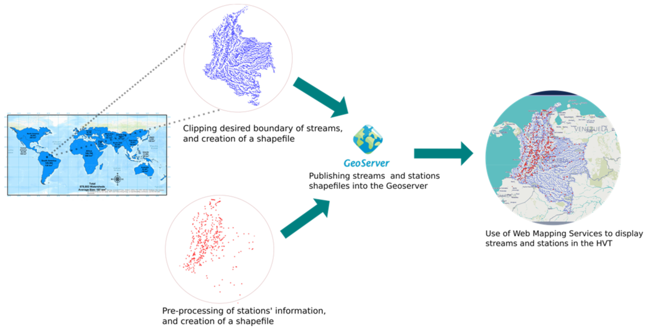
2.4. Spatial Data Pre-processing

The GESS provides historical streamflow simulations and short-term forecasts for the 13 regions in the world shown in Figure 1. To build a customized HVT for each of the five regions in our case studies, we first required the shapefiles that defined the streams in the regions of interest we had selected where GEOGloWS has computed global forecasts.

We obtained the shapefiles with the streams for the regions of interest from a public data resource in HydroShare [40]. We clipped the shapefile representing the streams to the country, watershed, or region of interest we had selected, as the GEOGloWS regional shapefiles covered significantly larger areas. Once clipped, we published the clipped shapefile to a GeoServer (Figure 2).

Next, we assigned each point in the gauging stations shapefile to its corresponding reach ID from the GESS model. This is a critical step in order to ensure that computed forecasts and observed data represent runoff from the same watershed. We assigned the gauging stations to their associated reach ID using a GIS spatial join operation. To perform this operation, we needed to be aware of the following issues:

• The location of the gauging stations is often not exact or does not match the river reach segments in the shapefile. Therefore, the locations should be visually examined and adjusted to match the right reach ID and location.
• The areas of the simulated basins are not the same as the area that corresponds to the basin defined by a gauging station point.

To address the first issue for our case studies, we discarded the stations that could not be adequately connected to a reach ID. This resulted in us retaining 412 of 656 original stations in Colombia, 303 of 400 stations in Peru, 82 of 84 stations in the Dominican Republic, 122 of 177 stations in Australia, and 1008 of 1019 stations in Brazil. After eliminating the gauging stations that could not be connected, we published the shapefile containing the gauging station locations to the same GeoServer in which we published the clipped stream network regions. The HVT application accesses this GeoServer to provide visualization of both the stream reaches with computed forecasts and the locations of gauging stations with observed data, all clipped to the boundary of the case study regions. The second issue was addressed using the bias correction described in Section 2.6, since the bias correction method takes into account not only the differences in the streamflow volume of the GESS model but also the differences in the area caused by the location of the gauging station.

Figure 2 shows an overview of this process. The top branch of the process diagram in Figure 2 shows the steps required for obtaining the stream reach segments with computed forecasts, while the bottom branch shows the steps for obtaining the gauging station locations. The right side of the figure shows how the GeoServer combined these two data sources into an integrated data set that we used to perform bias correction and model validation for each of our five regions.

2.5. Web Applicaation Design

The HVT application design consists of five main components that perform the following functions:

• retrieve data from mapping services for the stations and stream network in a region and present these data using a JavaScript map interface;
• retrieve, process, and visualize the simulated data (i.e., historical simulation and forecast) from the GEOGloWS or GESS servers;
• perform bias corrections on the historic simulation data using observed data;
• construct a bias-corrected forecast using the observed data and the historic simulated data; and
• compute and present comparisons and error metric reports of the historical simulation with and without the bias correction.

HVT presents visualization and data plotting using JavaScript functions. These visualizations include the retrieval of the gauges and clipped regions from the GeoServer via Web Map Service (WMS) and a presentation of the results using the HVT map interface. HVT uses these data to generate various plots and maps of different data such as observed, simulated, and bias-corrected streamflow to show both the data and present results visually for validation. HVT performs all the required back-end computations using Python functions and libraries. These back-end tasks include data retrieval and the processing of the hydrographs, the computing of analytical comparisons, bias correction, the generation of error metrics reports, and the construction of the corrected and updated forecasts.

The HVT map interface development was minimal compared to that of the back-end because the Tethys Platform gives the user an interface template that provides much of the framework for the interface. This meant that the HVT map interface development only required retrieval of the WMS and data plotting. The first part of the design required retrieval of the WMS in order to obtain the ID of the station and stream reach ID. Those ID’s were later used to retrieve the observed, historic simulated, corrected simulated, and forecast streamflow. The second part involved plotting the observed, simulated, and bias corrected data using the Plotly graphing library [41].

The HVT back-end includes functions for the processing and analysis of the observed, simulated, and bias-corrected data. These functions include analytical hydrograph comparisons, error metric calculations, and forward forecast adjustments for each station where observed data exist.

We created three different HVT functions to acquire the data and compute the hydrographs for the simulated, observed, and bias-corrected data. The first function uses the GESS REST API to retrieve the simulated data for the specific reach ID. The second function retrieves the observed data from the station associated with a reach ID. We modified this function for each regional app to use the appropriate service for retrieving observed data. For the countries that do not have their own service for providing observed hydrological data, we imported the data into resources that would provide standardized access. For the Dominican Republic we used the HydroServer Lite tool [42], while for Colombia and Peru we created HydroShare resources. The last function performs the bias correction of the simulated data using the observed data for the selected station following a variation of the method proposed by Farmer et al. [35]. HVT has a function that uses the data created by these functions (the simulated, observed and bias-corrected data) to plot the data with Plotly [41].

HVT computes an analytical comparison of the observed, simulated, and bias-corrected data using the HydroStats Python Package [34]. The HVT uses the following statistical visual analysis from the HydroStats python package: daily seasonality, monthly seasonality, and a scatter plot of predicted versus observed data in normal and log scales. We created a function in the back-end portion of HVT that uses the HydroStats package for each one of these statistical analyses to generate plots for the HVT web map interface. The daily and monthly average streamflow plots show how the bias-corrected streamflow captures the seasonality of the observed streamflow. The scatterplots show the distribution of the observed data compared to that of the simulated data. The scatter plot clearly shows the difference in alignment between the corrected data and the original simulated historical data with the observed data. HVT performs a volume analysis that computes a time series of the cumulative volume for the three different types of data and presents a plot and a table comparing the total volume for observed, simulated, and corrected flow.

HVT uses the HydroStats Python package [34] to create the error metrics report for the simulated and bias-corrected data. HydroStats contains tools used for calculating error metrics on observed and simulated time series and performs computations for forecast validation. The HydroStats package contains over 70 error metrics, with many specific to the field of hydrology. Application developers and users can select which metrics to activate. HydroStats provides the ability to present the selected metrics in a table, with two columns showing the difference in the error metrics for the historical simulated and historical bias-corrected data compared to the observed data, each selected error metric represented in a row. For the customized HVT applications used in our case studies, we chose a set of error metrics to build the error metric report. When customizing the HVT application, developers can choose to add additional metrics to the report from the HydroStats list. By default, the HVT application presents the following error metrics: mean error (ME) [43], root mean square error (RMSE) [32], normalized root mean squared error (NRMSE) [44], mean absolute percentage error (MAPE) [45], Nash–Sutcliffe model efficiency coefficient (NSE) [46], Kling–Gupta model efficiency coefficient (KGE) (2009), the modified KGE (2012) [47,48], Pearson correlation coefficient [49], Spearman’s rank correlation coefficient [50], and the coefficient of determination [51].

HVT uses two functions to construct the GESS and bias-corrected forecasts. The first function uses the GESS REST API to retrieve the forecast data for the specific reach ID associated with a station. The forecast displays the return periods values estimated from the GESS historic simulation if the forecast exceeds the 2-year return period threshold. The second function retrieves the bias-corrected forecast of the GESS forecast. It is bias-corrected using the observed data, the historic simulated data, and the method adopted from Farmer et al. [35]. Similarly, the bias corrected forecast displays the return periods values estimated from the bias corrected GESS historic simulation if the bias corrected forecast exceeds the 2-year return period threshold. Additionally, if the country, region, or watershed of interest provides a service with real-time observed data, an additional function to show the recently observed data can be included, allowing the users compare the magnitude of the forecast and the bias-corrected forecast with observed data.

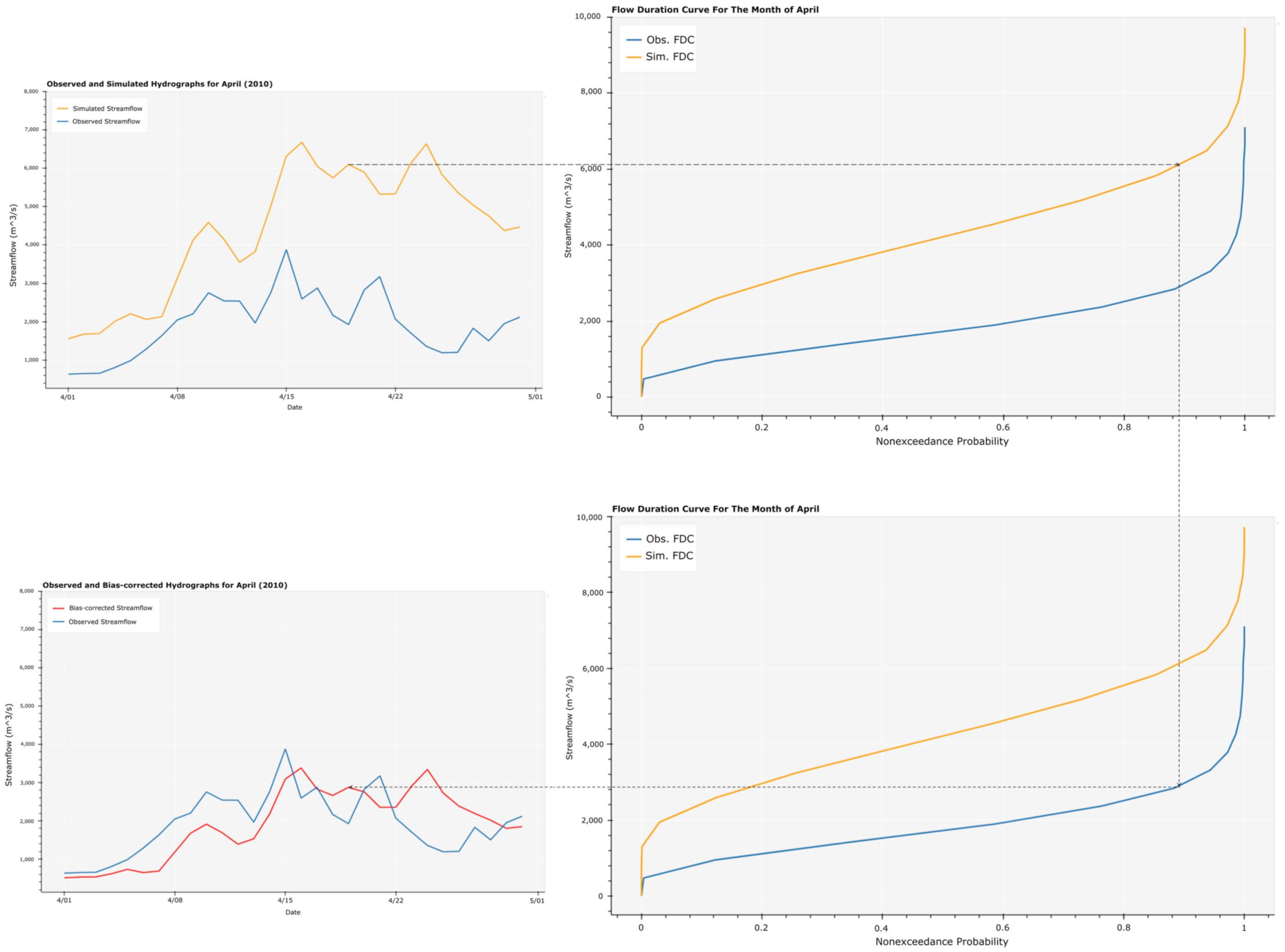
2.6. Bias Correction

The bias correction methodology we applied is based on the work of Farmer et al. [35]. Figure 3 shows the bias correction methodology we developed and applied. For every month in an observed and historic simulated time series, we calculate the flow duration curve. After that, in a single month, we can estimate the non-exceedance probability of every simulated value. Therefore, we can estimate the observed streamflow value that corresponds to that non-exceedance probability. Finally, we convert the simulated value by replacing it with the equivalent observed streamflow to the same non-exceedance probability.

Figure 4 shows how we extended the bias correction methodology applied for the historic simulation to the short-term forecast with the return period thresholds recalculated with the bias corrected historic simulation.

3. Results

In this section, we present results for both software implementation and case study hydrological results. We distribute our HVT implementation as an open source, web-based application that can be accessed freely from anywhere on the Internet to compute and retrieve bias-corrected forecasts. HVT needs to be customized for different regions to be able to access local observed data sources, or users can upload their own data to a HydroShare server if other services are not available. We provide the freely available source code to this web application on GitHub [52,53,54,55,56] where it can be downloaded, modified, and used by others.

We present the results of our experimental test cases in Australia, Brazil, Colombia, the Dominican Republic, and Peru. This presentation includes key error metrics displayed throughout the different stations across each of these study areas that show the improvement provided by the bias correction. Error metric results across each of the study areas before and after bias correction can be considered as calibration results, and the forecast result metrics evaluation can be considered a validation process. Unfortunately, the results of the bias correction methodology applied in the forecast were not evaluated. This paper is the first presentation of our implementation of the bias correction method, which is different from a calibration method because the model parameters are not being modified; instead, we modify the model results. We are currently further characterizing and testing this method and plan a future discussion of our bias correction method. The focus of this paper is the design, development, and testing of a web application framework that implements our bias correction method through the use of a web application and various services to facilitate the examination of a global streamflow system. The bias correction uses local data to correct these global simulation results so that they can be used more reliably to make decisions at local scale.

3.1. Software Implementation Results

The HVT web application provides users with access to:

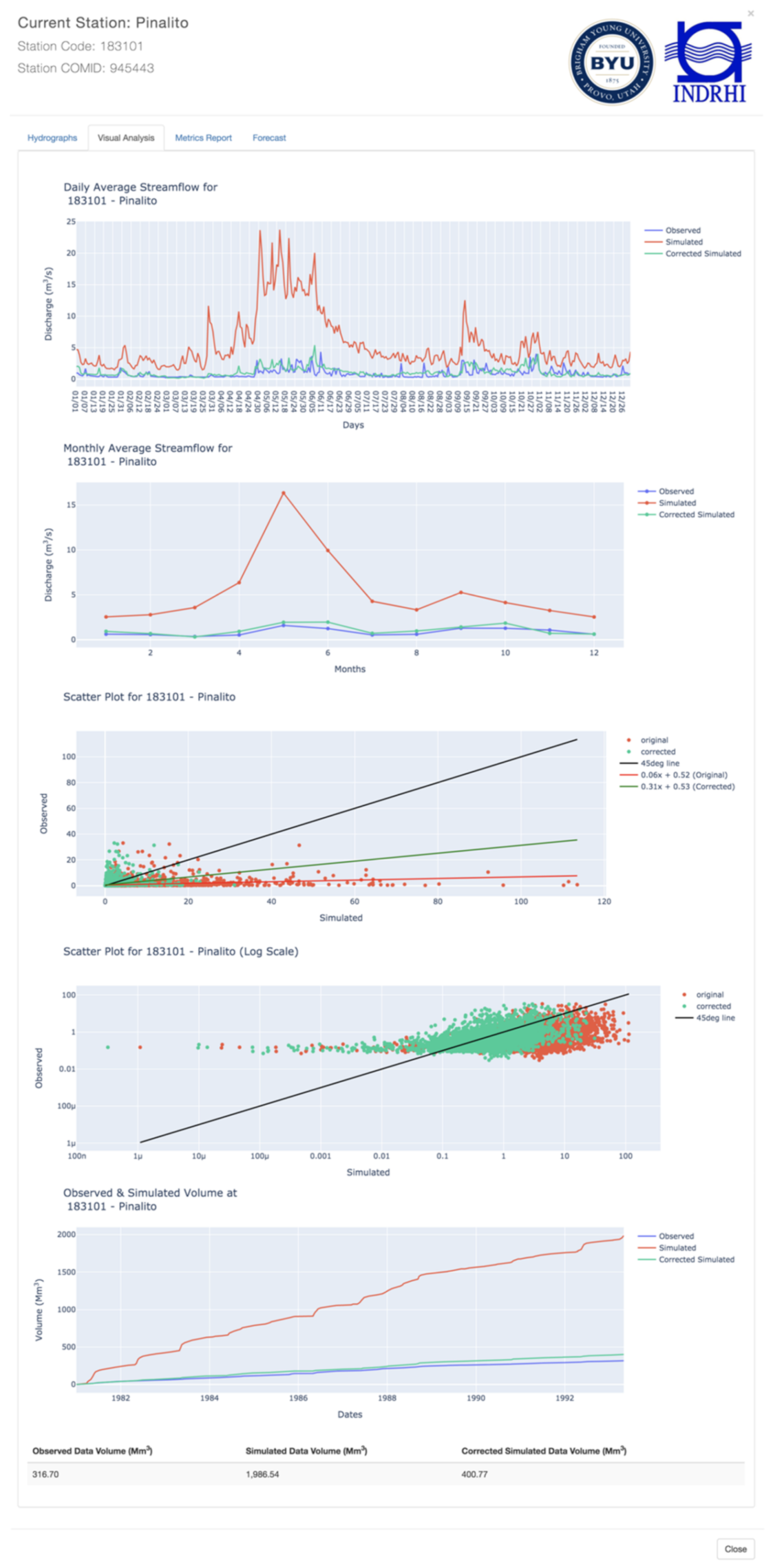
• Data and plots for the observed, simulated, and bias-corrected historic streamflow data;
• Visual analysis of daily seasonality, monthly seasonality, and scatter plots in normal and log scale;
• Computations and plots of volume analysis;
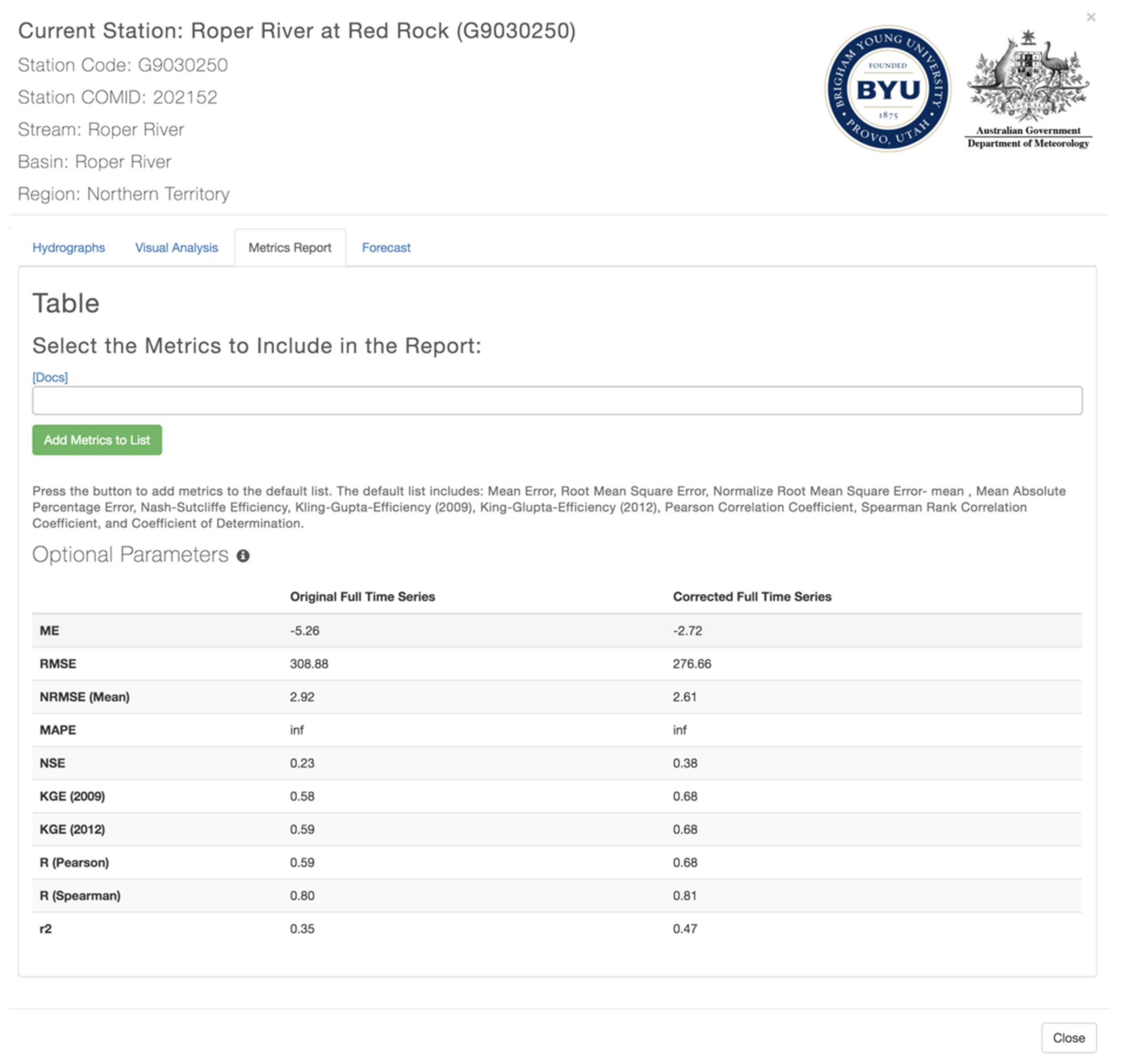
• Statistical error metrics validation for observed versus simulated and observed versus bias-corrected simulated data to evaluate the improvement from bias corrections; and
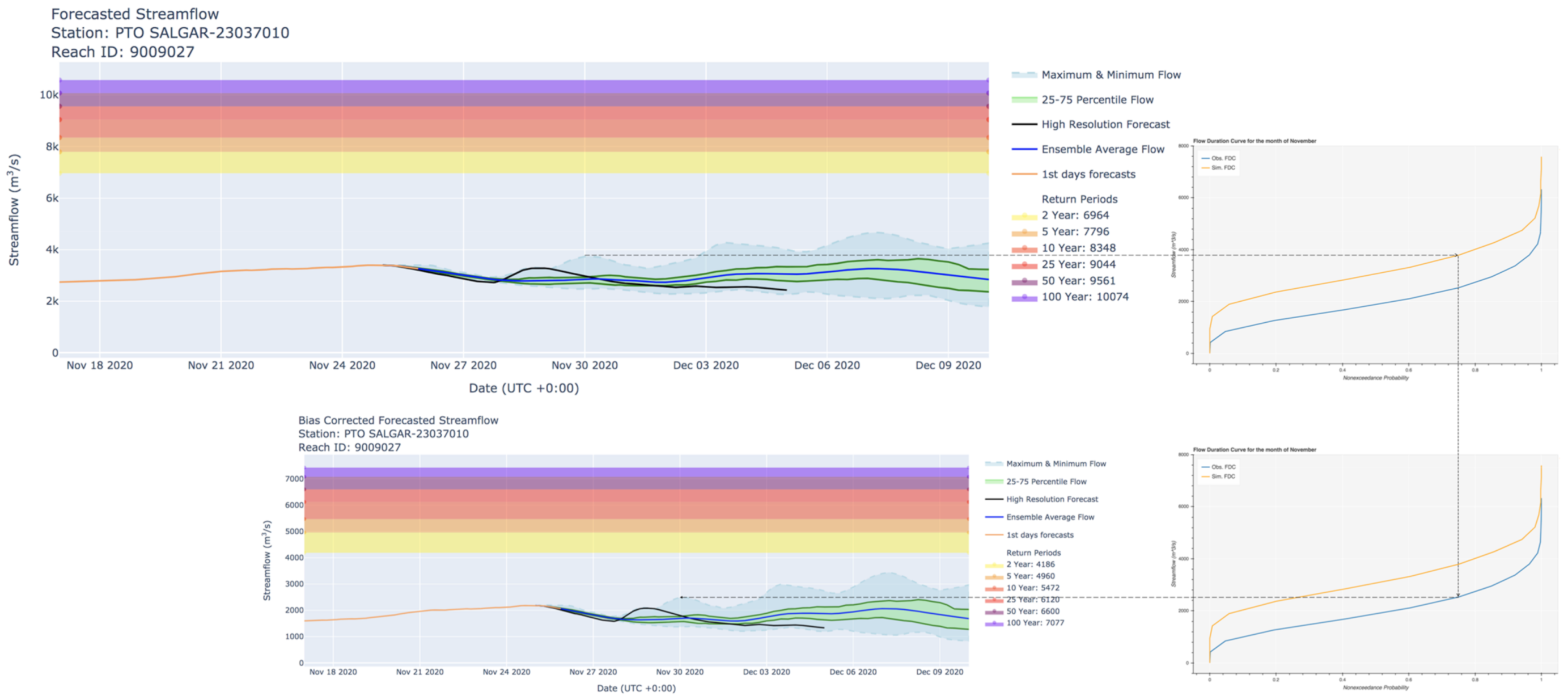
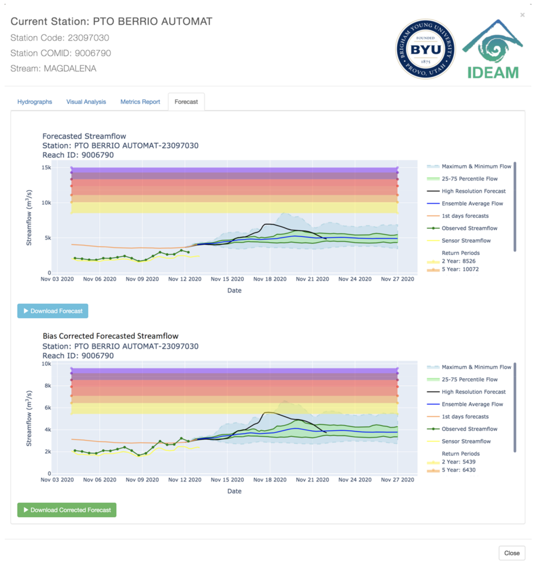
• Access to and visualizations of both the GESS hydrologic forecast and the bias-corrected forecast that can be used by local hydrological managers.

HVT performs all these functions so that users are not required to access or modify the original GESS model. HVT users do not need to interact with the GESS model’s developers to request changes, as HVT can perform validation and bias corrections for a local site or region using only local observed data.

The main page of the HVT web app (presented in Figure 5) shows the streams and stations for the country, watershed, or region of interest. Figure 5 shows the main page for the HVT customized for Brazil. The user interface for the Australia and the Dominican Republic HVT apps are very similar, just with a different region displayed.

On the main page, a user can select a gauge station and a pop-up with information about the selected station will appear with the following four tabs: hydrographs (Figure 6), the statistical visual analysis (Figure 7), the statistical metrics report (Figure 8), and the streamflow forecast (Figure 9). We will describe each of these tabs in detail below.

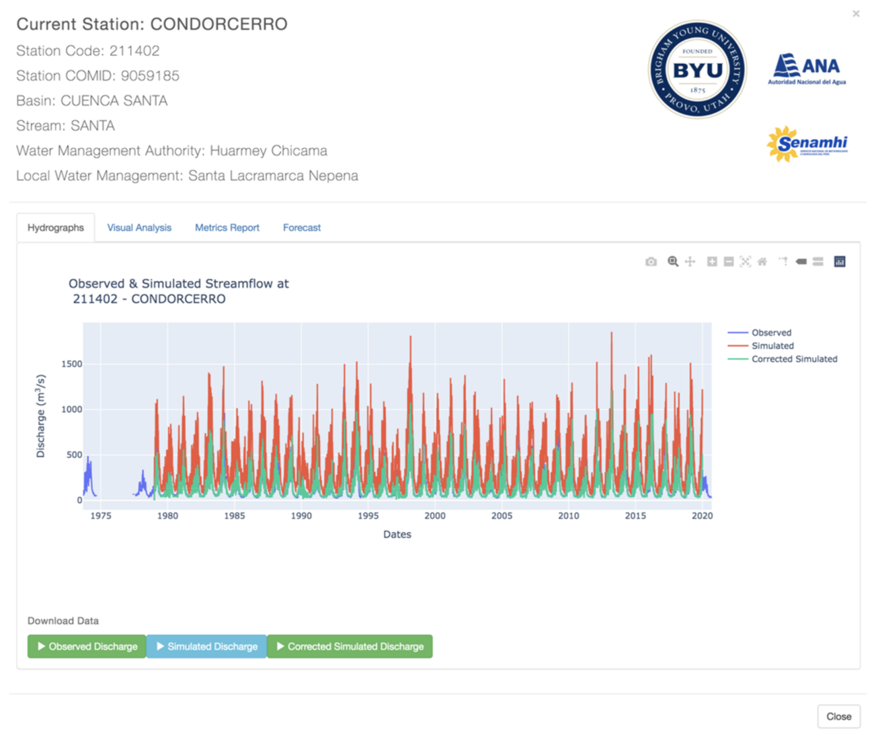
3.1.1. User Interface: Hydrographs

The first tab in the popup window is “Hydrographs.” Figure 6 shows this tab, which presents three hydrographs for the observed, simulated, and bias-corrected historical data. Figure 6 shows data from the Condorcerro Station in the Santa River in Peru. These plots show the improvement between the GESS historic simulated data (red) hydrograph and the bias-corrected data hydrograph (green). The improvement is easily noted, while it is difficult to distinguish between the observed (blue) and corrected simulated data (green). However, it is easy to distinguish between the observed (blue) or corrected (green), and simulated data (red). A user can toggle each hydrograph on and off for better understanding and confidence in the results. Users can also download the data for each one of the hydrographs if they require the data for additional analysis or use outside of HVT.

3.1.2. User Interface: Visual Analysis

The second tab in the popup window is “Visual Analysis.” Figure 7 shows this tab with the daily seasonality, monthly seasonality, scatter plots, volume analysis plot and volume analysis table for the Pinalito Station in the Dominican Republic. For example, the cumulative volume plot and table (bottom graph and table in the figure), shows that the corrected volume (400 Mm³) is closer to the observed volume (316.7 Mm³), than the simulated volume (1,985 Mm³) before the bias correction.

3.1.3. User Interface: Metrics Report

The third tab in the popup window is “Metrics Report.” Figure 8 shows the metric report of the Roper River at Red Rock station in Australia. The metrics report has a list of pre-determined metrics, but users can add additional metrics from those available in the HydroStats Package. This is done through a selection menu. The interface provides error metrics that can quantify the comparison and evaluation of improvement between the bias-corrected historical simulation and the original historical simulation according to the various error metrics. In the case shown in Figure 8, we can see that most of the metrics demonstrate an improvement after the bias correction (except for the MAPE metric). Since there are values of observed streamflow of 0.0 m³/s, the MAPE computation results in an infinite value.

3.1.4. User Interface: Forecast Visualization

The fourth tab in the popup window shows “Forecast Visualization.” Figure 9 shows the forecast for the Puerto Berrio station in the Magdalena River in Colombia. The tab displays the original forecast and bias-corrected forecast in the top and bottom plots, respectively. The top plot displays the original forecast before the bias correction, the return periods thresholds calculated from the historic simulation, and, for this station, the plot uses the real-time observed and sensor data from the Colombian hydrology and meteorology institute (IDEAM). The bottom forecast plot displays the biased corrected forecast, with return periods thresholds calculated from the bias corrected historic simulation, the real time observed, and the sensor data. For this station, the plots show how the bias correction appropriately adjusts the magnitude difference between the simulated and observed data. Both the original and corrected forecasts are downloadable.

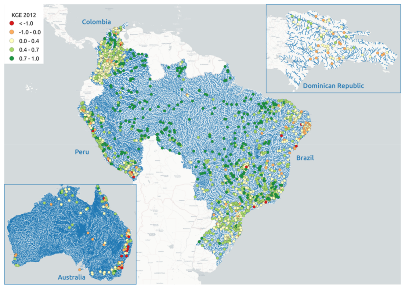
3.2. Experimental Case Study Results

We developed case studies of five country-wide analyses in Australia, Brazil, Colombia, the Dominican Republic, and Peru using the HVT. Each of these experimental cases use versions of the HVT web application customized to show the region of interest and access the observed data for that region. The main difference in the customizable applications is the source for the historic observed streamflow data and the real time observed streamflow data for each region. These sources are quite different, specifically:

• The Australia HVT application retrieved data using the web interface to the Bureau of Meteorology to access the daily streamflow data for the 122 gauging stations. For some of the stations, these data include real-time observed streamflow. HVT accesses these real-time data and uses them in the Forecast tab.
• The Brazil HVT application uses the open data portal of the National Water Agency to access the daily streamflow data for the 1008 gauging stations.
• The Colombia HVT application uses comma-separated-value (CSV) files for the observed data at each of the 412 stations. These data were provided by the Colombian Institute of Hydrology, Meteorology and Environmental Studies (IDEAM). To customize HVT, we grouped and added the observed streamflow CSV files for the 412 gauging stations in a HydroShare resource. The Colombia HVT application also uses the IDEAM Flood Early Warning System (FEWS) web service to retrieve the real time observed and sensor streamflow data that we added to the app in the Forecast section.
• The Dominican Republic HVT application uses an existing HydroServer to retrieve the observed data for each of the 84 gauging stations. The Dominican National Hydrologic service (INDRHI) provided the data on the HydroServer.
• The Peru HVT application uses CSV files for the observed data at each of the 303 stations. These data were provided by the Peruvian National Meteorology and Hydrology Service (SENAMHI). To customize HVT, we grouped and added the CSV files with the observed streamflow for the 303 gauging stations in a HydroShare resource.

While a full comparison of the bias correction method is not within the scope of this paper, here we present some common error metrics used in hydrology to compare how the bias correction method improved the historical simulation in the case studies. To evaluate the performance of the bias correction, we present the Kling–Gupta efficiency 2012 (KGE-2012) [48]. The KGE-2012 is a goodness-of-fit measure that provides a diagnostically interesting decomposition based on the NSE error metric.

For all five case studies, we can see an improvement in the bias-corrected historical simulation as measured by the KGE-2012 metric. These results are encouraging and suggest that this bias correction implemented in the HVT can be used to locally improve forecasts where historical observations are available.

Figure 10 shows a map of the KGE-2012 error metric computed for the original historical simulation and the observed data for Australia, Brazil, Colombia, the Dominican Republic, and Peru.

Figure 11 shows a map of the KGE-2012 error metric computed for the bias corrected historical simulation and the observed data for Australia, Brazil, Colombia, the Dominican Republic, and Peru. The KGE-2012 error metric showed some improvement between the original historical simulation and bias-corrected historical simulation in the five study cases (however, this improvement was shown at different levels).

The KGE-2012 error metric values for Australia show some improvement, especially in the western coast of Australia. The KGE-2012 error metric values become positive (signifying a lower error) after bias correction for most of the sites. However, some stations in the east coast of Australia did not show improvement, but rather the opposite. We think that this is due to an important number of big flow events that were not considered by the model or were represented with a time offset, causing the bias correction method to correct the magnitude of the streamflow peak, but not the time when the event occurred, introducing a penalty to the KGE-2012.

The KGE-2012 error metric value for the Dominican Republic showed significant improvement between the original historical simulation and the bias-corrected historical simulation. The KGE-2012 error metrics values after the bias correction become positive for most sites throughout the country. However, some stations in the country did not show improvement. Nearly all the stations without improvement were located in small rivers close to the coast, and the lack of improvement is similar to the situation explained for the stations in Australia case study.

The KGE-2012 error metric values for Brazil, Colombia, and Peru showed the most improvement from all the study cases. The bias-corrected historical simulation showed the largest improvement, especially in the Amazon region, while in the Andes region in Peru and Colombia and the east coast in Brazil, the improvement was not as apparent. Overall, most of the stations in Brazil, Colombia, and Peru showed significant improvement after we performed the bias correction.

4. Conclusions and Future Work

The combination of using hydrological modeling as a service, the availability of hydrological observation data as a web service, and statistical packages is essential to providing skillful and reliable global hydrological models for local use. With the HVT app, we offer a customizable web app that allows users access to observed streamflow data and simulated data from the GESS and other global models. The HVT bias correction method allows users to correct these global simulated data at the local scale. The use of HydroServer and HydroShare in sharing hydrological data improves the ability to automate a larger scale regional or national implementation. The HVT application can be adapted to different countries, hydrologic models, validation and bias correction methods, and sources of data. Users could also implement custom approaches for dealing with calibrated values, bias correction and other options.

An important capability that HVT provides is communication of the improvement in the simulated historical and forecasted streamflow using the bias correction. HVT presents an analysis of the historic simulation and bias corrected historical simulation data compared to observed data using reports and visualizations. These graphs and error metrics give users the confidence required to use global modeling results for local decisions. The HVT web app allows the use of local data to adjust forecasts. This makes global modeling results useful for their purposes at a local scale, without requiring them to adjust or calibrate the formulation of the original model. Since HVT is a web application, this also means that the application can be hosted remotely and does not require local users to obtain or maintain an expensive infrastructure.

Based on the results from the five case studies analyzed in this paper (Australia, Brazil, Colombia, the Dominican Republic, and Peru), we demonstrate that our streamflow bias correction method provided an effective way to use the results of a global model on a local scale. Bias correction generally improves the historic streamflow simulations. These results are encouraging and suggest that our bias correction method can be useful to locally improve forecasts. It provides local corrections that are an important element of local planning and decision making. Unfortunately, the HVT application can only provide bias-corrected values from the GESS in the places where observed information is available. Bias correction is provided only in the river reaches associated with a station. In addition, the bias correction method tends to not provide accurately results for big flow events that are not considered by the model or that have been considered with a time offset, as shown in the Australia and the Dominican Republic case studies.

We intend that future HVT releases to create warning points when the bias-corrected forecast exceeds the threshold defined by the return periods calculated using the bias-corrected historic simulation. Additionally, we will implement the HVT customization in more countries around the world and evaluate the improvement of the bias correction and what it provides for the historical simulation results. We plan to evaluate the performance of the GESS forecast before and after the bias correction in countries where recent observed streamflow data are available.

One of the main disadvantages of HVT is the inability to provide bias corrected data for ungauged basins. Therefore, it is important to develop methods to extrapolate the bias correction to ungauged basins through regionalization in order to take advantage of the ability of the GESS to retrieve hydrological modeling results in every stream in the world.

References

1. Jonkman, S.N. Global Perspectives on Loss of Human Life Caused by Floods. Nat. Hazards 2005, 34, 151–175. [Google Scholar] [CrossRef]
2. Pandey, S.; Bhandari, H. Drought: Economic costs and research implications. In Drought Frontiers in Rice; WORLD SCIENTIFIC: Singapore, 2009; pp. 3–17. ISBN 978-981-4280-00-6. [Google Scholar]
3. Snow, A. A New Global Forecasting Model to Produce High-Resolution Stream Forecasts. Master’s Thesis, Brigham Young University, Provo, UT, USA, 2015. [Google Scholar]
4. Souffront Alcantara, M.A. A Flexible Service-Oriented Approach to Address Hydroinformatic Challenges in Large-Scale Hydrologic Predictions. Ph.D. Thesis, Brigham Young University, Provo, UT, USA, 2018. [Google Scholar]
5. Pappenberger, F.; Ramos, M.H.; Cloke, H.L.; Wetterhall, F.; Alfieri, L.; Bogner, K.; Mueller, A.; Salamon, P. How do I know if my forecasts are better? Using benchmarks in hydrological ensemble prediction. J. Hydrol. 2015, 522, 697–713. [Google Scholar] [CrossRef] [Green Version]
6. Bartholmes, J.C.; Thielen, J.; Ramos, M.H.; Gentilini, S. The european flood alert system EFAS—Part 2: Statistical skill assessment of probabilistic and deterministic operational forecasts. Hydrol. Earth Syst. Sci. 2009, 13, 141–153. [Google Scholar] [CrossRef] [Green Version]
7. Thielen, J.; Bartholmes, J.; Ramos, M.-H.; de Roo, A. The European Flood Alert System—Part 1: Concept and development. Hydrol. Earth Syst. Sci. 2009, 13, 125–140. [Google Scholar] [CrossRef] [Green Version]
8. National Oceanic and Atmospheric Administration (NOAA). The National Water Model. Available online: https://water.noaa.gov/about/nwm (accessed on 13 May 2020).
9. National Oceanic and Atmospheric Administration (NOAA). NOAA Launches America’s First National Water Forecast Model|National Oceanic and Atmospheric Administration. Available online: https://www.noaa.gov/media-release/noaa-launches-america-s-first-national-water-forecast-model (accessed on 13 May 2020).
10. Cattoen, C.; McMillan, H.; Moore, S. Coupling a High-Resolution Weather Model with a Hydrological Model for Flood Forecasting in New Zealand. J. Hydrol. N. Z. 2016, 55, 1. [Google Scholar]
11. Kundzewicz, Z.W.; Jun, X. Towards an improved flood preparedness system in China. Hydrol. Sci. J. 2004, 49, 941–944. [Google Scholar] [CrossRef]
12. Robinson, J.; Perkins, J.; Quig, B. Hydrological Forecasting and Decision Making in Australia. 2015. Available online: https://es.slideshare.net/Delft_Software_Days/dsd-int-2015-hydrological-forecasting-and-decision-making-in-australia-justin-robinson-54944079 (accessed on 13 May 2020).
13. Yoshimura, K.; Ishitsuka, Y.; Hibino, K.; Yamazaki, D.; Yamamoto, K.; Kachi, M.; Oki, R. Development of Flood Forecasting System over Japan and Application to 2018 Japan Floods Event. In Proceedings of the 2019 European Geosciences Union General Assembly, EGU 2009, Vienna, Austria, 7–12 April 2019. [Google Scholar]
14. Alfieri, L.; Burek, P.; Dutra, E.; Krzeminski, B.; Muraro, D.; Thielen, J.; Pappenberger, F. GloFAS—Global ensemble streamflow forecasting and flood early warning. Hydrol. Earth Syst. Sci. 2013, 17, 1161–1175. [Google Scholar] [CrossRef] [Green Version]
15. Lavers, D.A.; Harrigan, S.; Andersson, E.; Richardson, D.S.; Prudhomme, C.; Pappenberger, F. A vision for improving global flood forecasting. Environ. Res. Lett. 2019, 14, 121002. [Google Scholar] [CrossRef] [Green Version]
16. The World Bank Group; Global Facility for Disaster Reduction and Recovery (GFDRR). Assessment of the State of Hydrological Services in Developing Countries 2018. Available online: https://www.gfdrr.org/sites/default/files/publication/state-of-hydrological-services_web.pdf (accessed on 29 January 2019).
17. Balsamo, G.; Beljaars, A.; Scipal, K.; Viterbo, P.; van den Hurk, B.; Hirschi, M.; Betts, A.K. A Revised Hydrology for the ECMWF Model: Verification from Field Site to Terrestrial Water Storage and Impact in the Integrated Forecast System. J. Hydrometeorol. 2009, 10, 623–643. [Google Scholar] [CrossRef]
18. Zsoter, E.; Wetterhall, F. GloFAS v2.1—Copernicus Services—ECMWF Confluence Wiki. Available online: https://confluence.ecmwf.int/display/COPSRV/GloFAS+v2.1 (accessed on 17 June 2020).
19. Harrigan, S.; Zsoter, E.; Alfieri, L.; Prudhomme, C.; Salamon, P.; Wetterhall, F.; Barnard, C.; Cloke, H.; Pappenberger, F. GloFAS-ERA5 Operational Global River Discharge Reanalysis 1979–Present. Earth Syst. Sci. Data Discuss. 2020, 12, 1–23. [Google Scholar] [CrossRef] [Green Version]
20. Snow, A.D.; Christensen, S.D.; Swain, N.R.; Nelson, E.J.; Ames, D.P.; Jones, N.L.; Ding, D.; Noman, N.S.; David, C.H.; Pappenberger, F.; et al. A High-Resolution National-Scale Hydrologic Forecast System from a Global Ensemble Land Surface Model. JAWRA J. Am. Water Resour. Assoc. 2016, 52, 950–964. [Google Scholar] [CrossRef] [Green Version]
21. Qiao, X.; Nelson, E.J.; Ames, D.P.; Li, Z.; David, C.H.; Williams, G.P.; Roberts, W.; Sánchez Lozano, J.L.; Edwards, C.; Souffront, M.; et al. A systems approach to routing global gridded runoff through local high-resolution stream networks for flood early warning systems. Environ. Model. Softw. 2019, 120, 104501. [Google Scholar] [CrossRef]
22. Souffront Alcantara, M.A.; Nelson, E.J.; Shakya, K.; Edwards, C.; Roberts, W.; Krewson, C.; Ames, D.P.; Jones, N.L.; Gutierrez, A. Hydrologic Modeling as a Service (HMaaS): A New Approach to Address Hydroinformatic Challenges in Developing Countries. Front. Environ. Sci. 2019, 7, 158. [Google Scholar] [CrossRef]
23. Hirpa, F.A.; Salamon, P.; Beck, H.E.; Lorini, V.; Alfieri, L.; Zsoter, E.; Dadson, S.J. Calibration of the Global Flood Awareness System (GloFAS) using daily streamflow data. J. Hydrol. 2018, 566, 595–606. [Google Scholar] [CrossRef]
24. Hales, R. Geoglows. Zenodo. 2020. Available online: https://doi.org/10.5281/zenodo.3891938 (accessed on 30 June 2020).
25. Chen, M.; Voinov, A.; Ames, D.P.; Kettner, A.J.; Goodall, J.L.; Jakeman, A.J.; Barton, M.C.; Harpham, Q.; Cuddy, S.M.; DeLuca, C.; et al. Position paper: Open web-distributed integrated geographic modelling and simulation to enable broader participation and applications. Earth-Sci. Rev. 2020, 207, 103223. [Google Scholar] [CrossRef]
26. Conner, L.G.; Ames, D.P.; Gill, R.A. HydroServer Lite as an open source solution for archiving and sharing environmental data for independent university labs. Ecol. Inform. 2013, 18, 171–177. [Google Scholar] [CrossRef]
27. Khattar, R.; Ames, D. A Web Services Based Water Data Sharing Approach Using Open Geospatial Consortium Standards. Open Water J. 2020, 6, 2. [Google Scholar]
28. Kadlec, J.; StClair, B.; Ames, D.P.; Gill, R.A. WaterML R package for managing ecological experiment data on a CUAHSI HydroServer. Ecol. Inform. 2015, 28, 19–28. [Google Scholar] [CrossRef]
29. Valentine, D.W.; Zaslavsky, I.; Whitenack, T.; Maidment, D. Design and Implementation of CUAHSI WaterML and WaterOneFlow Web Services. AGU Fall Meet. Abstr. 2007, 53, IN53C-08. [Google Scholar]
30. Tarboton, D.; Idaszak, R.; Horsburgh, J.; Heard, J.; Ames, D.; Goodall, J.; Band, L.; Merwade, V.; Couch, A.; Arrigo, J.; et al. HydroShare: Advancing Collaboration through Hydrologic Data and Model Sharing. In Proceedings of the International Congress on Environmental Modelling and Software, San Diego, CA, USA, 15–19 June 2014. [Google Scholar]
31. GeoServer GeoServer. GeoServer. 2020. Original Work Published 2011. Available online: https://github.com/geoserver/geoserver (accessed on 30 June 2020).
32. Dawson, C.W.; Abrahart, R.J.; See, L.M. HydroTest: Further development of a web resource for the standardised assessment of hydrological models. Environ. Model. Softw. 2010, 25, 1481–1482. [Google Scholar] [CrossRef]
33. Jackson, E.K.; Roberts, W.; Nelsen, B.; Williams, G.P.; Nelson, E.J.; Ames, D.P. Introductory overview: Error metrics for hydrologic modelling—A review of common practices and an open source library to facilitate use and adoption. Environ. Model. Softw. 2019, 119, 32–48. [Google Scholar] [CrossRef]
34. Roberts, W.; Williams, G.P.; Jackson, E.; Nelson, E.J.; Ames, D.P. Hydrostats: A Python Package for Characterizing Errors between Observed and Predicted Time Series. Hydrology 2018, 5, 66. [Google Scholar] [CrossRef] [Green Version]
35. Farmer, W.H.; Over, T.M.; Kiang, J.E. Bias correction of simulated historical daily streamflow at ungauged locations by using independently estimated flow duration curves. Hydrol. Earth Syst. Sci. 2018, 22, 5741–5758. [Google Scholar] [CrossRef] [Green Version]
36. Swain, N. Tethys Platform: A Development and Hosting Platform for Water Resources Web Apps. Ph.D. Thesis, Brigham Young University, Provo, UT, USA, 2015. [Google Scholar]
37. Nelson, E.J.; Pulla, S.T.; Matin, M.A.; Shakya, K.; Jones, N.; Ames, D.P.; Ellenburg, W.L.; Markert, K.N.; David, C.H.; Zaitchik, B.F.; et al. Enabling Stakeholder Decision-Making With Earth Observation and Modeling Data Using Tethys Platform. Front. Environ. Sci. 2019, 7. [Google Scholar] [CrossRef]
38. Jones, N.; Nelson, J.; Swain, N.; Christensen, S.; Tarboton, D.; Dash, P. Tethys: A Software Framework for Web-Based Modeling and Decision Support Applications. In Proceedings of the 8th International Congress on Environmental Modelling and Software: Bold Visions for Environmental Modeling, iEMSs 2014, San Diego, CA, USA, 15–19 June 2014. [Google Scholar]
39. Swain, N.R.; Christensen, S.D.; Snow, A.D.; Dolder, H.; Espinoza-Dávalos, G.; Goharian, E.; Jones, N.L.; Nelson, E.J.; Ames, D.P.; Burian, S.J. A new open source platform for lowering the barrier for environmental web app development. Environ. Model. Softw. 2016, 85, 11–26. [Google Scholar] [CrossRef] [Green Version]
40. Ashby, K. Derived Hydrography of World Regions 2020. Brigham Young University. Available online: https://doi.org/10.4211/hs.d5155cb57987489a95b83364d2c0f6c0 (accessed on 30 June 2020).
41. Plotly Technologies Inc. Collaborative Data Science; Plotly Technologies Inc.: Montréal, QC, Canada, 2015. [Google Scholar]
42. BYU-Hydroinformatics World Water—Historical Data. Available online: https://worldwater.byu.edu/historical-data (accessed on 30 June 2020).
43. Sammut, C.; Webb, G.I. (Eds.) Mean Error. In Encyclopedia of Machine Learning; Springer: Boston, MA, USA, 2010; p. 652-652. ISBN 978-0-387-30164-8. [Google Scholar]
44. Jain, A.; Srinivasulu, S. Integrated approach to model decomposed flow hydrograph using artificial neural network and conceptual techniques. J. Hydrol. 2006, 317, 291–306. [Google Scholar] [CrossRef]
45. Swamidass, P.M. (Ed.) MAPE (mean absolute percentage error) MEAN ABSOLUTE PERCENTAGE ERROR (MAPE). In Encyclopedia of Production and Manufacturing Management; Springer: Boston, MA, USA, 2000; p. 462-462. ISBN 978-1-4020-0612-8. [Google Scholar]
46. Nash, J.E.; Sutcliffe, J.V. River flow forecasting through conceptual models part I—A discussion of principles. J. Hydrol. 1970, 10, 282–290. [Google Scholar] [CrossRef]
47. Gupta, H.V.; Kling, H.; Yilmaz, K.K.; Martinez, G.F. Decomposition of the mean squared error and NSE performance criteria: Implications for improving hydrological modelling. J. Hydrol. 2009, 377, 80–91. [Google Scholar] [CrossRef] [Green Version]
48. Kling, H.; Fuchs, M.; Paulin, M. Runoff conditions in the upper Danube basin under an ensemble of climate change scenarios. J. Hydrol. 2012, 424–425, 264–277. [Google Scholar] [CrossRef]
49. Kirch, W. (Ed.) Pearson’s Correlation Coefficient. In Encyclopedia of Public Health; Springer Netherlands: Dordrecht, The Netherlands, 2008; pp. 1090–1091. ISBN 978-1-4020-5614-7. [Google Scholar]
50. Dodge, Y. Spearman Rank Correlation Coefficient. In The Concise Encyclopedia of Statistics; Springer: New York, NY, USA, 2008; pp. 502–505. ISBN 978-0-387-32833-1. [Google Scholar]
51. Dodge, Y. Coefficient of Determination. In The Concise Encyclopedia of Statistics; Springer: New York, NY, USA, 2008; pp. 88–91. ISBN 978-0-387-32833-1. [Google Scholar]
52. BYU-Hydroinformatics. Historical_Validation_Tool_Australia; BYU Hydroinformatics Lab, 2021. Original Work Published 2019. Available online: https://github.com/BYU-Hydroinformatics/historical_validation_tool_australia (accessed on 5 February 2021).
53. BYU-Hydroinformatics. Historical_Validation_Tool_Brazil; BYU Hydroinformatics Lab, 2021. Original Work Published 2020. Available online: https://github.com/BYU-Hydroinformatics/historical_validation_tool_brazil (accessed on 5 February 2021).
54. BYU-Hydroinformatics. Historical_Validation_Tool_Colombia; BYU Hydroinformatics Lab, 2021. Original Work Published 2019. Available online: https://github.com/BYU-Hydroinformatics/historical_validation_tool_colombia (accessed on 5 February 2021).
55. BYU-Hydroinformatics. Historical_Validation_Tool_Dominican_Republic; BYU Hydroinformatics Lab, 2021. Original Work Published 2019. Available online: https://github.com/BYU-Hydroinformatics/historical_validation_tool_dominican_republic (accessed on 5 February 2021).
56. BYU-Hydroinformatics. Historical_Validation_Tool_Peru; BYU Hydroinformatics Lab, 2021. Original Work Published 2020. Available online: https://github.com/BYU-Hydroinformatics/historical_validation_tool_peru (accessed on 5 February 2021).
Figure 1. GEOGloWS Global Streamflow Prediction Tool World Regions.
Hydrology 08 00071 g001
Figure 2. Preprocessing of the streams and gauging stations for their use. The left side of the figure shows the data sources for the stream reaches and associated computed forecasts (top) and the gauging stations and associated observed data (bottom). The circled data represents the clipping of the data sources to the region of interest. These clipped data are then uploaded to the GeoServer, which provides access to the combined data.
Hydrology 08 00071 g002
Figure 3. The bias correction methodology we developed for the GESS historic simulation, based on Farmer et al. [35].
Hydrology 08 00071 g003
Figure 4. Plots showing data corrected using the correction methodology we developed for the GESS forecast.
Hydrology 08 00071 g004
Figure 5. Main page for the historical validation tool app for Brazil.
Hydrology 08 00071 g005
Figure 6. Hydrographs tab for the Condorcerro Station in the Historical Validation Tool App for Peru.
Hydrology 08 00071 g006
Figure 7. Visual analysis for the Pinalto station in the historical validation tool app for the Dominican Republic.
Hydrology 08 00071 g007
Figure 8. Metrics report for the Roper River at Red Rocks (G9030250) station for the HVT App for Australia.
Hydrology 08 00071 g008
Figure 9. Forecast for the Puerto Berrio automatic station in the historical validation tool app for Colombia.
Hydrology 08 00071 g009
Figure 10. KGE-2012 error metric computed for the difference between the original historical simulation and the observed data for Australia, Brazil, Colombia, the Dominican Republic, and Peru.
Hydrology 08 00071 g010
Figure 11. KGE-2012 error metric between the bias-corrected historical simulation and the observed data for Australia, Brazil, Colombia, the Dominican Republic, and Peru.
Hydrology 08 00071 g011
Publisher’s Note: MDPI stays neutral with regard to jurisdictional claims in published maps and institutional affiliations.