Modelling Long-Term Monthly Rainfall Variability in Selected Provinces of South Africa: Trend and Extreme Value Analysis Approaches

Abstract

Extreme rainfall events have made significant damages to properties, public infrastructure and agriculture in some provinces of South Africa notably in KwaZulu-Natal and Gauteng among others. The general global increase in the frequency and intensity of extreme precipitation events in recent years is raising a concern that human activities might be heavily disturbed. This study attempts to model long-term monthly rainfall variability in the selected provinces of South Africa using various statistical techniques. The study investigates the normality and stationarity of the underlying distribution of the whole body of rainfall data for each selected province, the long-term trends of the rainfall data and the extreme value distributions which model the tails of the rainfall distribution data. These approaches were meant to help achieve the broader purpose of this study of investigating the long-term rainfall trends, stationarity of the rainfall distributions and extreme value distributions of monthly rainfall records in the selected provinces of South Africa in this era of climate change. The five provinces considered in this study are Eastern Cape, Gauteng, KwaZulu-Natal, Limpopo and Mpumalanga. The findings revealed that the long-term rainfall distribution for all the selected provinces does not come from a normal distribution. Furthermore, the monthly rainfall data distribution for the majority of the provinces is not stationary. The paper discusses the modelling of monthly rainfall extremes using the non-stationary generalised extreme value distribution (GEVD) which falls under the block maxima extreme value theory (EVT) approach. The maximum likelihood estimation method was used to obtain the estimates of the parameters. The stationary GEVD was found as the best distribution model for Eastern Cape, Gauteng, and KwaZulu-Natal provinces. Furthermore, model fitting supported non-stationary GEVD model for maximum monthly rainfall with nonlinear quadratic trend in the location parameter and a linear trend in the scale parameter for Limpopo, while in Mpumalanga the non-stationary GEVD model with a nonlinear quadratic trend in the scale parameter and no variation in the location parameter fitted well to the monthly rainfall data. The negative values of the shape parameters for Eastern Cape and Mpumalanga suggest that the data follow the Weibull distribution class, while the positive values of the shape parameters for Gauteng, KwaZulu-Natal and Limpopo suggest that the data follow the Fréchet distribution class. The findings from this paper could give information that can assist decision makers establish strategies for proper planning of agriculture, infrastructure, drainage system and other water resource applications in the South African provinces.

1. Introduction

According to [1], climate change is possibly the biggest environmental problem facing the globe. Masereka et al. [2] stated that flood risks are caused by extreme rainfall events that have resulted in flood disasters that accounted for about 47% of all weather-related calamities, affecting 2.3 billion people worldwide. In the past decades, extreme precipitation events have made significant damages to properties, public infrastructure, agriculture, finance and tourism in the Hawaiian Islands [3].

Muchuru et al. [4] stated that Southern Africa is a region of high rainfall variability and is disposed to serious events such as floods and droughts. Recent increases in the frequency and intensity of extreme rainfall events have raised concern that human activities might have resulted in a change of the climate system [5]. On the contrary, [6] argued that there is a growing concern in Southern Africa about the declining rainfall patterns as a result of global warming. Manhique et al. [7] reported that the flood that occurred in January 2013 left almost 20,000 people homeless and about 100 dead in central and southern parts of Mozambique.

South Africa is classified as a predominantly semi-arid country. The climate of South Africa ranges from desert and semi-desert in the dry north-western region to sub-humid and wet along the eastern coastal area [8]. According to [1], South Africa is a water-stressed country with high spatio-temporal rainfall variability. This climate variability in South Africa is a result of the location of South Africa in the tropical and subtropical zones. South Africa has nine provinces, namely: Eastern Cape, Free State, Gauteng, KwaZulu-Natal, Limpopo, Mpumalanga, Northern Cape, North-West and Western Cape. The present study is carried out in the provinces of Eastern Cape, Gauteng, KwaZulu-Natal, Limpopo and Mpumalanga.

According to [9], KwaZulu-Natal is the wettest province of South Africa, with rainfall along the northeast coast exceeding 1300 mm per annum, but declining to 800 mm per annum inland. Dyson [10] stated that Gauteng province receives most of its rainfall in summer months, with the north-western part of the province obtaining rainfall more frequently as compared to the south and south-east part of the province. A study conducted by [11] showed no significant trend, but increases in summer rainfall and decreases in autumn and winter rainfall in KwaZulu-Natal. Thomas et al. [12] observed an increase in early-season rainfall and a decrease in late-season rainfall in north-west KwaZulu-Natal for the period 1950–2000. In the same study, [12] found a tendency for a later seasonal rainfall onset accompanied by increased dry spells and fewer rain days in the Limpopo province. Rainfall variability in the Eastern Cape province causes water reduction in reservoirs [13]. Oduniyi [14] highlighted that over the past decade in Mpumalanga province, there has been occurrence of climate change such as excessive temperature, fire outbreaks, rainfall and floods which caused a damage to agricultural productions. The Western Cape has been impacted by severe storms occurring almost annually over the past two decades, resulting in damages to homes, agricultural produces and infrastructure [15].

The present study seeks to model long-term monthly rainfall variability in selected provinces of South Africa using time series and extreme value theory (EVT) approaches. Results from this study can contribute positively to the body of knowledge in EVT application to rainfall data and recommendations will be suggested to the government agencies on the long-term rainfall variability and their negative impact on the economy. To the best of our knowledge, there are no studies available on the public domain that have modelled long-term monthly rainfall variability in these selected provinces of South Africa using the trend analysis and EVT approaches employed in this present study.

2. Materials and Methods

2.1. Data Source and Study Area

Aggregated provincial monthly rainfall data from 1900 to 2017 for the five selected provinces of South Africa were obtained from the South African Weather Service (SAWS) and the secondary data were time series measured in millimeters (mm). Two provinces, Limpopo and Mpumalanga, had monthly rainfall data for the period 1904–2017, while the rest of the provinces had monthly rainfall data from 1900 to 2017.

2.2. Test for Stationarity

Statistical theory offers a wide range of unit root tests, with the most commonly used being augmented Dickey-Fuller (ADF) test, Phillips-Perron (PP) test and Kwiatkowski-Phillips-Schmidt-Shin (KPSS) test [16]. In this study ADF, PP and KPSS are used to test whether the monthly rainfall data for selected provinces of South Africa are stationary.

2.2.1. Augmented Dickey-Fuller (ADF) Test

The ADF test was employed in this study to check whether the monthly rainfall data for selected provinces of South Africa are stationary.

The ADF test is assessed under the following hypotheses:

H${}_{\mathbf{0}}$: There exists a unit root and the time series is non-stationary,

H${}_{\mathbf{1}}$: The time series is stationary.

The ADF test consists of estimating the following regression model:

$$y_t=\beta +{\beta }_{1}t+\delta Y_{t-1}+\sum _{i=1}^m{\alpha }_i△Y_{t-1}+{ϵ}_t,$$

(1)

where $\beta$ is a constant, ${\beta }_1$ is the coefficient on time trend. The null hypothesis is $\delta =1$, and the alternative hypothesis is $\delta \ne 1$, while ${ϵ}_t$ is a pure white noise error term and the ADF follows an asymptotic distribution [17].

2.2.2. Phillips-Perron (PP) Unit Root Test

The Phillips-Perron test is a more developed test, introduced in 1988 and it has the same null hypothesis with ADF test and also uses the same critical values with it [18,19]. The PP test makes a non-parametric correction to the t-statistic. The PP test involves the equation coming from Dickey-Fuller test:

$$△Y_t=\mu +v+{\lambda }_t+{ϵ}_t,$$

(2)

where ${ϵ}_t$ is I(0) and it can be heteroscedastic. For this reason, the test estimates the equation:

$$y_t=y_{t-1}+v+{\lambda }_t+{ϵ}_t.$$

(3)

The PP method estimates the non-augmented DF test equation and modifies the t-ratio of the coefficient, so that serial correlation does not affect the asymptotic distribution of the test statistic. The PP test is based on the statistic:

$${\overline{t}}_{\mu }=t_{\mu }{\left({\displaystyle \frac{{\gamma }_0}{f_0}}\right)}^{\frac{1}{2}}-\frac{T(f_0-{\gamma }_0\left[se\left(\mu \right)\right]}{2f_0^{\frac{1}{2}}s}.$$

(4)

The PP test is assessed under the following hypotheses:

H${}_{\mathbf{0}}$: There is a unit root,

H${}_{\mathbf{1}}$: There is no unit root.

2.2.3. Kwiatkowski-Phillips-Schmidt-Shin (KPSS)

The ADF and PP test mentioned in the previous sections are testing the null hypothesis that the time series $y_t$ is integrated of order one, $I\left(1\right)$. The opposite case, that is, testing the null hypothesis that the time series $y_t$ is $I\left(0\right)$ is described by the KPSS test [20]. KPSS builts on the idea that the time series is stationary around a deterministic trend and is calculated as the sum of deterministic trend, random walk and stationary random error. It is based on the model:

$$\begin{array}{c}\hfill y_t=d_t+r_t+{ϵ}_t,\\ \hfill r_t=r_{t-1}+u_t,\end{array}$$

(5)

where $d_t={\sum }_{i=o}^p{\beta }_i{t}^i$, for $p=0,1$, contains deterministic parts of the model constant or deterministic trend, ${ϵ}_t$ are independent and identically distributed (iid) error terms $\sim N(0,{\sigma }_{ϵ}^2$), and $r_t$ is a random walk with variance ${\sigma }_u^2$ and $u_t$. KPSS test is based on the likelihood method test of the hypothesis that random walk has a zero variance, i.e., H${}_0$:${\sigma }_u^2$ = 0, which means that $r_t$ is a constant, against the alternative H${}_1$:${\sigma }_u^2$> 0. The test statistic is written as:

$$LM=\sum _{t=1}^T{s}_t^2/\widehat{{\sigma }_{ϵ}},$$

(6)

where $s_t$ = ${\sum }_{t=1}^T\widehat{ϵ}$, $t=1,2,...,T$, and $\widehat{{\sigma }_{ϵ}^2}$ is the estimate of variance ${\sigma }_{ϵ}^2$ of process ${ϵ}_t$ from Equation (5). Critical values are derived by a simulation method and are listed in [20]. The advantage of the KPSS is that to some extent KPSS alleviates the problem that is present with the ADF test [21].

Kwiatkowski et al. [20] argue that KPSS test can differentiate a series that appears to be stationary, series that appears to have a unit root, and series for which the data are not sufficiently informative to be sure whether they are stationary or integrated.

The KPSS test is assessed under the following hypotheses:

H${}_{\mathbf{0}}$: The series does not have a unit root or is stationary,

H${}_{\mathbf{1}}$: The series has a unit root or is not stationary.

2.3. Trend Test

This study used non-parametric Mann-Kendall (M-K) test statistic, Sen’s slope estimator and time series plots to investigate the long-term trend of the monthly rainfall and its variability across the selected provinces.

2.3.1. Non-Parametric Mann-Kendall (M-K) Test Statistic

The non-parametric Mann-Kendall (M-K) test statistic is frequently used to quantify the significance of monotonic trend in hydrometeorological time series [22,23]. The M-K test statistic is defined as

$$S=\sum _{j=1}^{n-1}\sum _{i=j+1}^n\mathrm{sgn}(e_i-e_j),$$

(7)

where n is the number of extreme values. If S is positive, then there is an increasing trend, but if S is negative, then there is a decreasing trend, and $\mathrm{sgn}(e_i-e_j)$ is a sign function given by:

$$\mathrm{sgn}(e_i-e_j)=\left\{\begin{array}{cc}1,\hfill & \mathrm{if}{e}_i-e_j>0,\hfill \\ 0,\hfill & \mathrm{if}{e}_i-e_j=0,\hfill \\ -1.\hfill & \mathrm{if}{e}_i-e_j<0.\hfill \end{array}\right.$$

(8)

Under the null hypothesis of no trend, the theoretical mean of S is 0 and its variance is given by

$$Var\left(S\right)=\left[n(n-1)(2n+5)-\sum _{p=1}^g{t}_p(t_p-1)(2t_p+5)\right]/18,$$

(9)

where g is the number of tied groups (a tied group is a set of sample data having the same value), and $t_p$ is the number of data points in the pth tied group. If no tied group exist, this process can be ignored [23]. In cases where the sample size $n>30$, the normalised test statistic Z can be used to statistically quantify the significance of the trend. Z is calculated using the following equation:

$$Z=\left\{\begin{array}{cc}\frac{S-1}{\sqrt{Var\left(S\right)}},\hfill & \mathrm{if}S>0,\hfill \\ 0,\hfill & \mathrm{if}S=0,\hfill \\ \frac{S+1}{\sqrt{Var\left(S\right)}},\hfill & \mathrm{if}S<0.\hfill \end{array}\right.$$

(10)

Positive values of Z indicate an increasing trend, while negative Z values show decreasing trends. In a one-tailed test at a significance level of $\alpha$, the null hypothesis of no trend is rejected if $\mid Z\mid$ > $z_{\alpha }$, where z is the standard normal variable. In this study, the significance level was set to be 5%.

2.3.2. Sen’s Slope Estimator

Sen’s slope estimator non-parametric method was used to estimate the magnitude of trends in the time series data [24]. The slope of “n” pairs of data can be first estimated by using the following equation:

$${\beta }_i=Median\left[\frac{X_j-X_k}{j-k}\right]\forall k<j.$$

(11)

In this equation, $X_j$ and $X_k$ denote data values at time j and k, respectively, and time j is after time k$(k\le j)$. The median of “n” values of ${\beta }_i$ is the Sen’s slope estimator test. A negative ${\beta }_i$ value represents a decreasing trend, a positive ${\beta }_i$ value represents an increasing trend over time.

If “n” is an even number, then the Sen’s slope estimator is computed by using the following equation:

$${\beta }_{med}=\frac{1}{2}({\beta }_{[n/2]}+{\beta }_{\left[\right(n+2)/2]}).$$

(12)

If “n” is an odd number, then the estimated slope by using the Sen’s slope method can be computed as follows:

$${\beta }_{med}=\left({\beta }_{[n+/2]}\right).$$

(13)

${\beta }_{med}$ is tested by a two tailed test at 100 (1$-\alpha$) % confidence level, and the true slope of monotonic trend can be estimated by using a non-parametric test [25,26].

2.3.3. Time Series Plots

A time series plot is simply a graph in which the data values are arranged sequentially in time. It is commonly used to give a pictorial view of the data series over time.

2.4. Test for Normality

According to [27], there are several parametric and non-parametric methods of assessing whether data are normally distributed or not. These methods can be split into two groups: graphical and statistical. The most frequently used methods include: Quantile-quantile (Q-Q) plots, density plots, probability-probability (P-P) plots, Anderson–Darling test (AD), Shapiro–Wilk (SW) test, D’Agostino-Pearson K2 (DPK) test, chi-square test, Jarque-Bera (JB) test, kurtosis test, Shapiro-Francia (SF), skewness test, robust Jarque-Bera (RJB) test among others. In this study the JB, SW and chi-square methods are employed to check whether the monthly rainfall data are normally distributed. The SW test is one of the most popular tests for normality assumption diagnostics, and has good properties of power based on correlation within given observations and associated normal scores [28]. The JB and chi-square tests are among the most widely used techniques for testing normality of the data.

2.4.1. Jarque-Bera (JB) Test

The JB test statistic is expressed as:

$$JB=n\left(\frac{{\left(\sqrt{b_1}\right)}^2}{6}+\frac{{(b_2-3)}^2}{24}\right),$$

(14)

where $\sqrt{b_1}$ and $b_2$ are the skewness and kurtosis measures and are given by $\frac{m_3}{{\left(m_2\right)}^{3/2}}$ and $\frac{m_4}{{\left(m_2\right)}^3}$, respectively; and $m_2$, $m_3$ and $m_4$, are second, third and fourth central moments, respectively. The JB test statistic is chi-square distributed with two degrees of freedom.

The hypothesis test for the JB test procedure is

H${}_{\mathbf{0}}$: The monthly rainfall data is normally distributed, versus,

H${}_{\mathbf{1}}$: The monthly rainfall data do not come from a normal distribution.

2.4.2. Shapiro–Wilk (SW) Test

The SW test is of the form:

$$W=\frac{1}{D}{\left[\sum _{i=1}^m{a}_i(x_{(n-i+1)}-x_{\left(i\right)}\right]}^2,$$

(15)

where $m=\frac{n}{2}$ if n is even, while $m=\frac{(n-1)}{2}$ if n is odd. $D={\sum }_{i=1}^n{(x_i-\overline{x})}^2$ and $x_{\left(i\right)}$ represent the $i^{th}$ order statistic of a sample. The constants $a_i$ are given by:

$(a_1,a_2,...,a_n)=\frac{m^T{V}^{-1}}{{\left(m^T{V}^{-1}{V}^{-1}m\right)}^{\frac{1}{2}}}$ and m is given by $m={(m_1,m_2,...,m_n)}^T$, where $m_1,m_2,...,$

$m_n$ are the expected values of order statistics of iid random variables sampled from the standard normal distribution, and V is the covariance matrix of those order statistics [27].

The SW test is assessed under the following hypotheses:

H${}_{\mathbf{0}}$: The monthly rainfall data is normally distributed,

H${}_{\mathbf{1}}$: The monthly rainfall data does not come from a normal distribution.

2.4.3. Chi-Square Test

The chi-square goodness-of-fit test is defined as:

$${\chi }^2=\sum _{i=1}^n\frac{{(O_i-E_i)}^2}{E_i},$$

(16)

where $\left(O_i\right)$ and $\left(E_i\right)$ refer to the ith observed and expected frequencies, respectively, and n is the number of groups. When the null hypothesis is true, the above test statistic follows a chi-square distribution with $k-1$ degrees of freedom [27].

The chi-square test is assessed under the following hypotheses:

H${}_{\mathbf{0}}$: The monthly rainfall data are sampled from a normal distribution,

H${}_{\mathbf{1}}$: The monthly rainfall data are not sampled from a normal distribution.

2.5. Extreme Value Theory Techniques

In extreme value theory (EVT) two approaches exist: the block maxima (BM) and the peaks-over-threshold (POT) methods. According to [29], the BM is an approach in EVT that consists of dividing the observation period into non-overlapping periods of equal sizes. The current study utilises the BM approach in a changing climate to model monthly rainfall of the five selected provinces of South Africa.

2.5.1. Stationary Generalised Extreme Value Distribution

Generalised extreme value distribution (GEVD) is the family of asymptotic distribution that describes the behaviour of extreme conditions. The GEVD consists of three extreme value distributions namely: Gumbel, Fréchet and Weibull families which are also referred to as type I, II and III extreme value distributions [30,31,32]. The cumulative probability distribution for GEVD is of the form:

$$GEV(x,\mu ,\sigma ,\xi )=\left\{\begin{array}{c}exp-{\left[1+\xi \left(\frac{x-\mu }{\sigma }\right)\right]}^{\frac{-1}{\xi }};\xi \ne 0,\hfill \\ exp\left(-exp\left(-\frac{x-\mu }{\sigma }\right)\right);\xi =0,\hfill \end{array}\right.$$

(17)

where x are the extreme values from the blocks, $\mu$, $\sigma$ and $\xi$ are the location, scale and shape parameters, respectively. For $\xi >0$, we obtain the Fréchet distribution, for $\xi =0$, we get the Gumbel distribution and for $\xi <0$, we get the Weibull distribution.

2.5.2. Non-Stationary Generalised Extreme Value Distribution

The non-stationary GEVD model is the fundamental modification of the stationary GEVD model [30]. To account for non-stationary GEVD, the location parameter $\mu$ and the scale parameter $\sigma$ are assumed to vary with time t and possibly other covariates [32,33]. The non-stationary GEVD is given by:

$$GEVD(x;\mu \left(t\right),\sigma \left(t\right),\xi \left(t\right)=exp-{\left[1+\xi \frac{x-\mu \left(t\right)}{\sigma \left(t\right)}\right]}^{-\frac{1}{\xi \left(t\right)}},\xi \ne 0.$$

(18)

In the simplest case, the following regression structures could be examined for the location and scale parameters:

$$\mu \left(t\right)={\mu }_0+{\mu }_{1}t+{\mu }_2{t}^2,$$

(19)

$$\sigma \left(t\right)=exp({\sigma }_0+{\sigma }_{1}t+{\sigma }_2{t}^2,$$

(20)

$$\xi \left(t\right)=\xi ,$$

(21)

allowing up to quadratic dependence on time t and keeping the shape parameter constant [34].

2.5.3. Parameter Estimation of Non-Stationary GEVD

Parameters of the non-stationary GEVD are estimated using the method of maximum likelihood (ML). For a sample of N observations, the ML of the time-dependent GEVD in (18) was determined by maximising the log-likelihood function, expressed with time-varying parameters:

$$\begin{array}{cc}\hfill l\left(\mu \right(t),\sigma (t),\xi )& =-\sum _{t=1}^{N}log\sigma \left(t\right)+\left(1+\frac{1}{\xi }\right)log\left[1+\xi \left(\frac{x_i-\mu \left(t\right)}{\sigma \left(t\right)}\right)\right]\hfill \\ \hfill & +{\left[1+\xi \left(\frac{x_i-\mu \left(t\right)}{\sigma \left(t\right)}\right)\right]}^{-1/\xi },\hfill \end{array}$$

(22)

where N is the number of years of observation. To obtain the GEVD parameter estimators that maximise Equation (18) we use the interior algorithm based nonlinear optimisation in the MATLAB Optimisation Toolbox [22].

2.6. Goodness-of-Fit

Goodness-of-fit test statistics are used for checking the validity of a specified or assumed probability distribution model. In this study, Kolmogorov-Smirnov (K-S) test, Anderson-Darling (A-D) and graphical methods, were applied to identify the best model.

2.6.1. Kolmogorov-Smirnov (K-S) Test

The K-S test, based on the empirical cumulative distribution function is used to decide if a sample comes from a hypothesised continuous distribution [35,36,37]. The K-S statistic D is defined as the largest vertical distance between theoretical and the empirical cumulative distribution (CDF) and is formulated as follows:

$$D_{max}=\underset{1\le i\le n}{max}\left(F\left(x_i\right)-\frac{i-1}{n};\frac{i}{n}-F\left(x_i\right)\right),$$

(23)

where $X_i$ are random samples, $i=1,2,...,n$, and the CDF is

$$F_n\left(x\right)=\frac{1}{n}\left[Numberofobservations\le x\right].$$

(24)

The K-S test is estimated under the following hypotheses:

H${}_{\mathbf{0}}$: The monthly rainfall data follow a specified distribution,

H${}_{\mathbf{1}}$: The monthly rainfall data do not follow the specified distribution.

2.6.2. Anderson-Darling (A-D) Test

The A-D test statistic $\left(A^2\right)$ is defined as:

$$A^2=-n-\frac{1}{n}\sum _{i=1}^n\left(2i-1\right)\left[lnF\left(X_i\right)+ln(1-F\left(X_{n-i+1}\right))\right].$$

(25)

The A-D test is used to compare the fit of an observed CDF to an expected CDF. This test gives more weight to the tails of the distribution than the K-S test [36,37].

The A-D test is estimated under the following hypotheses:

H${}_{\mathbf{0}}$: The monthly rainfall data follow a specified distribution,

H${}_{\mathbf{1}}$: The monthly rainfall data do not follow the specified distribution.

2.6.3. Graphical Test

Alam et al. [35] stated that graphical test is one of the most simple powerful techniques for selecting the best-fit model. To check if the time-dependent GEVD fit well to the monthly rainfall data, the following graphical tests were used.

Quantile-quantile (Q-Q) plots

Quantile-quantile (Q-Q) plot, is a comparison of an empirical form for estimating the exceedance and the inverse of fitted distribution function. Any departure from linearity indicates model failure in perfectly fitting the data [38].

Probability-probability (P-P) plots

Probability-probability (P-P) plot is a comparison of an empirical (usually percentage rank) and the fitted distribution function. In case of perfect fit, the data would line up on the diagonal of the probability plots [35,38].

Return level plots

In these plots the empirical estimates of the return level functions are added. If there is an agreement between the model-based curve and empirical estimates, then the model is suitable for the data [35,38].

2.6.4. Choice of Preferred Model

When time-dependent GEVD is considered with covariates, there are a number of possible models to select from [39]. In order to select between model fits, a test of the likelihood ratio test also known as the deviance (D) statistic is used. For models $M_0\subset M_i$, we define the D statistic as:

$$D=2\left\{l_i\left(M_i\right)-l_0\left(M_0\right)\right\},i=1,2,3,...$$

(26)

where $l_0\left(M_0\right)$ and $l_i\left(M_i\right)$ are the maximised log-likelihood under models $M_0$ and $M_i$, respectively. The asymptotic distribution of D is given by ${\chi }_k^2$ distribution with k degrees of freedom, where k is the difference in dimensionality of $M_i$ and $M_0$. The calculated deviance statistic, D, is compared to critical values from ${\chi }_k^2$ at $\alpha$ level of significance. Large values of D suggest that $M_i$ explains substantially more of the variation in the data than $M_0$ [32] and [39].

3. Exploratory Data Analysis

This section is divided into three sections: descriptive statistics, stationarity tests and normality tests.

3.1. Descriptive Statistics

The descriptive statistics evaluated are the mean, standard deviation, median, kurtosis, skewness, minimum and the maximum monthly rainfall amount for each province. The summary of the descriptive statistics for each province is presented in

Table 1. Descriptive statistics of the monthly rainfall data.

Provinces	Min	Max	Median	Mean	Std.dev	Kurt	Skew
Eastern Cape	0.50	211.00	42.50	49.03	34.46	4.06	0.99
Gauteng	0.01	438.10	45.45	58.45	55.62	5.22	1.18
KwaZulu-Natal	0.01	478.80	67.75	73.92	57.23	5.68	1.10
Limpopo	1.00	112.00	45.00	46.74	31.40	1.93	0.26
Mpumalanga	1.00	111.00	47.00	48.19	31.28	1.85	0.16

Note: Min = Minimum, Max = Maximum, Std.dev = Standard deviation, Kurt = Kurtosis, Skew = Skewness.

.

From Table 1, the monthly rainfall data for each province has a mean value $\overline{X}>Q_2$ (Median), indicating that the monthly rainfall data is positively skewed and this is confirmed by the positive values of skewness. Eastern Cape, Gauteng, KwaZulu-Natal provinces have kurtosis greater than three which indicate heavy tails than a normal distribution, while Limpopo and Mpumalanga have kurtosis less than three which indicate lighter tails than a normal distribution.

The standard deviation for all the five provinces ranges from 31.28 to 57.23 mm per month. KwaZulu-Natal province has the highest standard deviation with the value of 57.23 mm per month which indicates a large variation in the monthly rainfall series, while Mpumalanga province has the lowest standard deviation of 31.28 mm per month which implies a small variation in the monthly rainfall series.

The minimum monthly rainfall ranges between 0.01 mm and 0.50 mm per month where Eastern Cape receives the highest minimum rainfall of 0.50 mm per month, while Gauteng and KwaZulu-Natal receive the lowest minimum rainfall of 0.01 mm per month.

The maximum monthly rainfall lie between 111.00 mm and 478.80 mm per month where KwaZulu-Natal receives the highest maximum monthly rainfall of 478.80 mm per month followed by Gauteng with the maximum rainfall of 438.10 mm per month. Mpumalanga receives the lowest maximum rainfall of 111.00 mm per month.

3.2. Test for Stationarity Results

The augmented Dickey-Fuller(ADF), Phillips-Perron (PP) and Kwiatkowski-Phillips-Schmidt-Shin (KPSS) tests were used to check for stationarity of monthly rainfall data for selected provinces of South Africa.

Table 2. ADF, KPSS and PP stationarity test results of monthly rainfall data.

Provinces	Test	Test Statistic	p-Value
Eastern Cape	ADF	−3.7614	0.02092
	KPSS	3.7258	0.01
	PP	−1432	0.01
Gauteng	ADF	−2.6238	0.3143
	KPSS	4.205	0.01
	PP	−840.85	0.01
KwaZulu-Natal	ADF	−2.6452	0.3052
	KPSS	4.1714	0.01
	PP	−1003.5	0.01
Limpopo	ADF	−7.1461	0.01
	KPSS	1.8398	0.01
	PP	−1502.6	0.01
Mpumalanga	ADF	−8.1155	0.01
	KPSS	0.96204	0.03041
	PP	−1312.9	0.010

shows the results of the ADF, PP and KPSS tests.

The ADF and PP tests were assessed under the following hypotheses:

H${}_{\mathbf{0}}$: There exists a unit root and the time series is non-stationary,

H${}_{\mathbf{1}}$: The time series is stationary.

The KPSS test was tested under the following hypotheses:

H${}_{\mathbf{0}}$: The series does not have a unit root test (or series is stationary).

H${}_{\mathbf{1}}$: The series has a unit root (or series is not stationary).

From Table 2 the p-values of the ADF test statistics for Eastern Cape, Limpopo and Mpumalanga are significant (p < 0.05), suggesting that the monthly rainfall data for these three provinces are stationary. The ADF p-values for Gauteng and KwaZulu-Natal are insignificant (p> 0.05), suggesting that the monthly rainfall data for these two provinces are not stationary at 5% level of significance.

Also, from Table 2 the p-values of the KPSS test for all five provinces are significant (p < 0.05), suggesting that the monthly rainfall data are not stationary. Furthermore, from Table 2 the p-values of the PP test for all five provinces are significant (p< 0.05), implying that the monthly rainfall data are stationary.

Overall, based on all the stationarity test findings, we conclude that the monthly rainfall data are not stationary for the majority of the provinces.

3.3. Test for Normality Results

In this study we formally tested for normality of the monthly rainfall data using the Jarque-Bera (JB), Shapiro-Wilk (SW) and chi-square tests.

Table 3. JB, SW and chi-square normality test results of monthly rainfall data.

Provinces	Test	Test Statistic	p-Value
Eastern Cape	JB	298.15	<0.01
	SW	0.93113	<0.01
	Chi-square	34276	<0.01
Gauteng	JB	618.22	<0.01
	SW	0.88137	<0.01
	Chi-square	78541	<0.01
KwaZulu-Natal	JB	710.9	<0.01
	SW	0.92103	<0.01
	Chi-square	62693	<0.01
Limpopo	JB	83.244	<0.01
	SW	0.9511	<0.01
	Chi-square	29843	<0.01
Mpumalanga	JB	83.833	<0.01
	SW	0.95219	<0.01
	Chi-square	28739	<0.01

, presents the results of the normality tests.

The JB, SW and chi-square tests are assessed under the following hypotheses:

H${}_{\mathbf{0}}$: The monthly rainfall data are normally distributed, versus,

H${}_{\mathbf{1}}$: The monthly rainfall data do not come from a normal distribution.

From Table 3, the results for all the three normality tests are significant (p < 0.05), which suggests that the monthly rainfall data for all the five provinces do not come from a normal distribution.

4. Results and Discussion

This section is divided into two sections namely; trend analysis and model fitting.

4.1. Trend Analysis Results

Mann-Kendall test statistic, Sen’s slope estimator and time series plots were used to analyse the long-term trends of the monthly rainfall data for the five provinces. The Mann-Kendall test statistic and Sen’slope results are presented in

Table 4. Results for Mann-Kendall test statistic and Sen’s slope estimator.

Provinces	M-K Test Statistic	Kendall’s Tau ($\mathit{\tau }$)	p-Value	Sen’s Slope
Eastern Cape	−4.130	−0.073	0.01	−0.009
Gauteng	−3.057	−0.054	0.002	−0.008
KwaZulu-Natal	−2.399	−0.043	0.016	−0.009
Limpopo	−0.832	−0.015	0.405	−0.002
Mpumalanga	−0.487	−0.009	0.626	0.000

. The outcome of the Mann-Kendall test results revealed that in Eastern Cape, Gauteng and KwaZulu-Natal provinces there were significant monotonic decreasing long-term trends (p < 0.05 and $\tau$ negative), while in Limpopo and Mpumalanga there were no significant monotonic decreasing long-term trends (p > 0.05 and $\tau$ negative). Sen’s slope values for Eastern Cape, Gauteng and KwaZulu-Natal showed significant decreasing magnitudes of trends, which were corresponding with the Mann-Kendall test results. While in Limpopo, Sens’ slope value revealed an insignificant decreasing magnitude of trend, which also supports the findings from Mann-Kendall test. On the other hand, Sen’s slope value for Mpumalanga showed no magnitude of trend, which slightly differs from the results of Mann-Kendall test. The latter findings illustrate the insignificance of the decreasing monotonic trend for Mpumalanga.

Figure 1 illustrate the monthly rainfall data time series plots for Eastern Cape, Gauteng, KwaZulu-Natal, Limpopo and Mpumalanga provinces. The time series plots in Figure 1 do not exhibit any significant discernible long-term trends for all the provinces. This justifies the use of Mann-Kendall test to help uncover the hidden long-term trends in the monthly rainfall series in Table 4.

4.2. Non-Stationary GEVD Modelling of Annual Block Maxima Rainfall Data

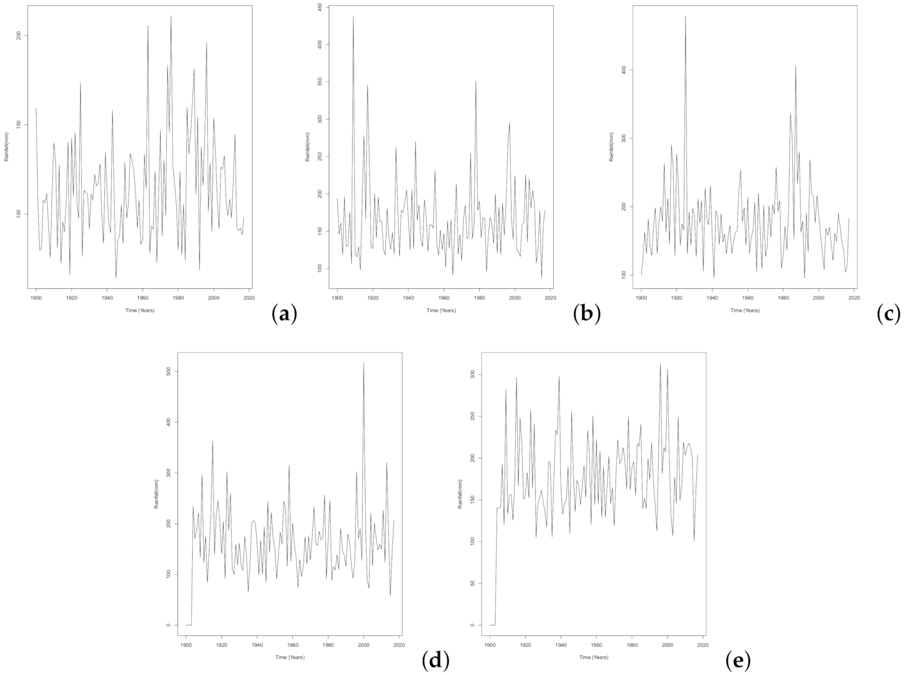
The time series plots of the annual block maxima rainfall series are shown in Figure 2. There seems to be some strong evidence for a positive long-term trend over the years, for all the provinces. A substantial part of the variability in the data can probably be explained by a systematic variation in rainfall over the years. One way of capturing this trend is by allowing the GEVD location and scale parameters to vary with time [40]. From Figure 2 a simple linear trend in time seems plausible for our annual maximum rainfall $X_t$, and we can use the model

$$X_t\sim GEV(\mu \left(t\right),\sigma \left(t\right),\xi ),$$

(27)

where $\mu \left(t\right)$ and $\sigma \left(t\right)$ are the time-dependent location and scale parameters, respectively.

In the present study, eight models are proposed for the non-stationary GEVD: $M_1,M_2,$ $M_3,M_4,M_5,M_6,M_7$ and $M_8$. The reference model is denoted by $M_0$ and is the stationary GEVD [40]. Model $M_1$ has a linear trend in the location parameter such that $\mu \left(t\right)={\mu }_0+{\mu }_{1}t$, $\sigma \left(t\right)=\sigma$ and $\xi \left(t\right)=\xi$; Model $M_2$ has a linear trend in the scale parameter such that $\mu \left(t\right)=\mu$, $log\sigma \left(t\right)=exp({\sigma }_0+{\sigma }_{1}t)$ and $\xi \left(t\right)=\xi$; Model $M_3$ has a linear trend in both location and scale parameters such that $\mu \left(t\right)={\mu }_0+{\mu }_{1}t$, $log\sigma \left(t\right)=exp({\sigma }_0+{\sigma }_{1}t)$ and $\xi \left(t\right)=\xi$; Model $M_4$ has a nonlinear quadratic trend in the location parameter and a linear trend in scale parameter such that $\mu \left(t\right)={\mu }_0+{\mu }_{1}t+{\mu }_2{t}^2$, $log\sigma \left(t\right)=exp(\sigma +{\sigma }_{1}t)$ and $\xi \left(t\right)=\xi$; Model $M_5$ has a linear trend in the location parameter and a nonlinear quadratic trend in the scale parameter such that $\mu \left(t\right)={\mu }_0+{\mu }_{1}t$, $log\sigma \left(t\right)=exp({\sigma }_0+{\sigma }_{1}t+{\sigma }_2{t}^2)$ and $\xi \left(t\right)=\xi$; Model $M_6$ has a nonlinear quadratic trend in both location and scale parameters such that $\mu \left(t\right)={\mu }_0+{\mu }_{1}t+{\mu }_2{t}^2$, $log\sigma \left(t\right)=exp({\sigma }_0+{\sigma }_{1}t+{\sigma }_2{t}^2)$ and $\xi \left(t\right)=\xi$; Model $M_7$ has a nonlinear quadratic trend in the location parameter with no variation in scale such that $\mu \left(t\right)={\mu }_0+{\mu }_{1}t+{\mu }_2{t}^2$, $\sigma \left(t\right)=\sigma$ and $\xi \left(t\right)=\xi$; Model $M_8$ has a nonlinear quadratic trend in the scale parameter with no variation in the location parameter such that $\mu \left(t\right)=\mu$, $log\sigma \left(t\right)=exp({\sigma }_0+{\sigma }_{1}t+{\sigma }_2{t}^2)$ and $\xi \left(t\right)=\xi$.

4.2.1. Eastern Cape

The stationary GEVD model for Eastern Cape data (i.e., model $M_0$) has a maximum negative log-likelihood (NLLH) of 556.765 (see

Table 5. Non-stationary GEVD models for Eastern Cape for the period 1900–2017.

Model	$\widehat{{\mathit{\mu }}_0}$	$\widehat{{\mathit{\mu }}_1}$	$\widehat{{\mathit{\mu }}_2}$	$\widehat{{\mathit{\sigma }}_0}$	$\widehat{{\mathit{\sigma }}_1}$	$\widehat{{\mathit{\sigma }}_2}$	$\widehat{\mathit{\xi }}$	NLLH
$M_0$	100.782	0	0	23.244	0	0	−0.012	556.769
$M_1$	95.768	0.086	0	23.057	0	0	−0.013	555.820
$M_2$	100.7005	0	0	22.328	0.017	0	−0.019	556.724
$M_3$	94.955	0.102	0	20.715	0.041	0	−0.022	555.530
$M_4$	98.043	−0.039	0.001	20.928	0.036	0	−0.010	555.837
$M_5$	99.323	0.002	0	18.126	0.310	−0.003	0.092	556.543
$M_6$	96.672	−0.003	0.001	17.7333	0.246	−0.002	0.095	556.084
$M_7$	98.475	−0.033	0.001	22.982	0	0	−0.002	556.048
$M_8$	99.499	0	0	18.263	0.305	−0.003	0.091	556.592

Key: NLLH = negative log-likelihood.

). A GEVD model with linear trend in the location parameter (i.e., $M_1$) has a maximum NLLH of 555.820. The deviance statistic for comparing these two models is therefore, D = 2(556.769 − 555.820) = 1.898, which is small compared to ${\chi }_1^2\left(0.05\right)=3.841$. Thus, allowing for a linear trend in the location parameter does not improve on our stationary GEVD model, $M_0$. Therefore, $M_1$ is not a worth model to consider.

Consider the pair of models $(M_0,M_2)$ from Table 5. The deviance statistic is 2(556.769 − 555.724) = 2.090, which is small compared to ${\chi }_1^2\left(0.05\right)=3.841$. Thus, allowing for a linear trend in the scale parameter does not improve on our stationary GEVD model, therefore, we reject model $M_2$ and conclude that is not worthwhile to allow for a linear trend in the scale parameter.

From Table 5, the deviance statistics of model pairs $(M_0,M_3)$ and $(M_0,M_7)$ are 2.478 and 1.442, respectively. Since both values of the deviance statistics are smaller than ${\chi }_2^2\left(0.05\right)=5.991$, it implies that both models do not provide any improvement in fit over the stationary GEVD model. The other model pairs from Table 5 $(M_0,M_4)$ and $(M_0,M_5)$, have deviance statistics of 1.864 and 0.452, respectively. These results revealed that model $M_4$, which allows for nonlinear quadratic trend in the location parameter and a linear trend in the scale parameter, does not provide an improvement in fit over the stationary GEVD model since the value of the deviance statistic (1.864) is small as compared to the value of ${\chi }_3^2\left(0.05\right)=7.815$. Also, model $M_5$, which allows for linear trend in location parameter and a nonlinear quadratic trend in the scale parameter, does not provide an improvement in fit over the stationary GEVD model since the value of the deviance statistic is smaller than the value of ${\chi }_3^2\left(0.05\right)=7.815$.

The nonlinear quadratic model pair $(M_0,M_6)$, which allows for nonlinear quadratic trend in both location and scale parameters, does not improve the stationary GEVD model since the deviance statistic, D = 1.37, is very small compared to ${\chi }_4^2\left(0.05\right)=9.488$. Again in Table 5, the model pair $(M_0,M_8)$, which allows for nonlinear quadratic trend in scale parameter with no variation in location parameter, has a deviance statistic of 0.354, which is too small compared to the critical value of 5.991 with 2 degrees of freedom. Thus, allowing for a quadratic trend in the scale parameter with no variation in the location parameter does not improve on the stationary GEVD.

Overall, the final model for Eastern Cape is the stationary GEVD model, $M_0$. The general model for Eastern Cape is given by

$$GEVD(x,\mu ,\sigma ,\xi )=exp-{\left[1-0.012\left(\frac{x-100.782}{23.244}\right)\right]}^{\frac{1}{0.012}}.$$

(28)

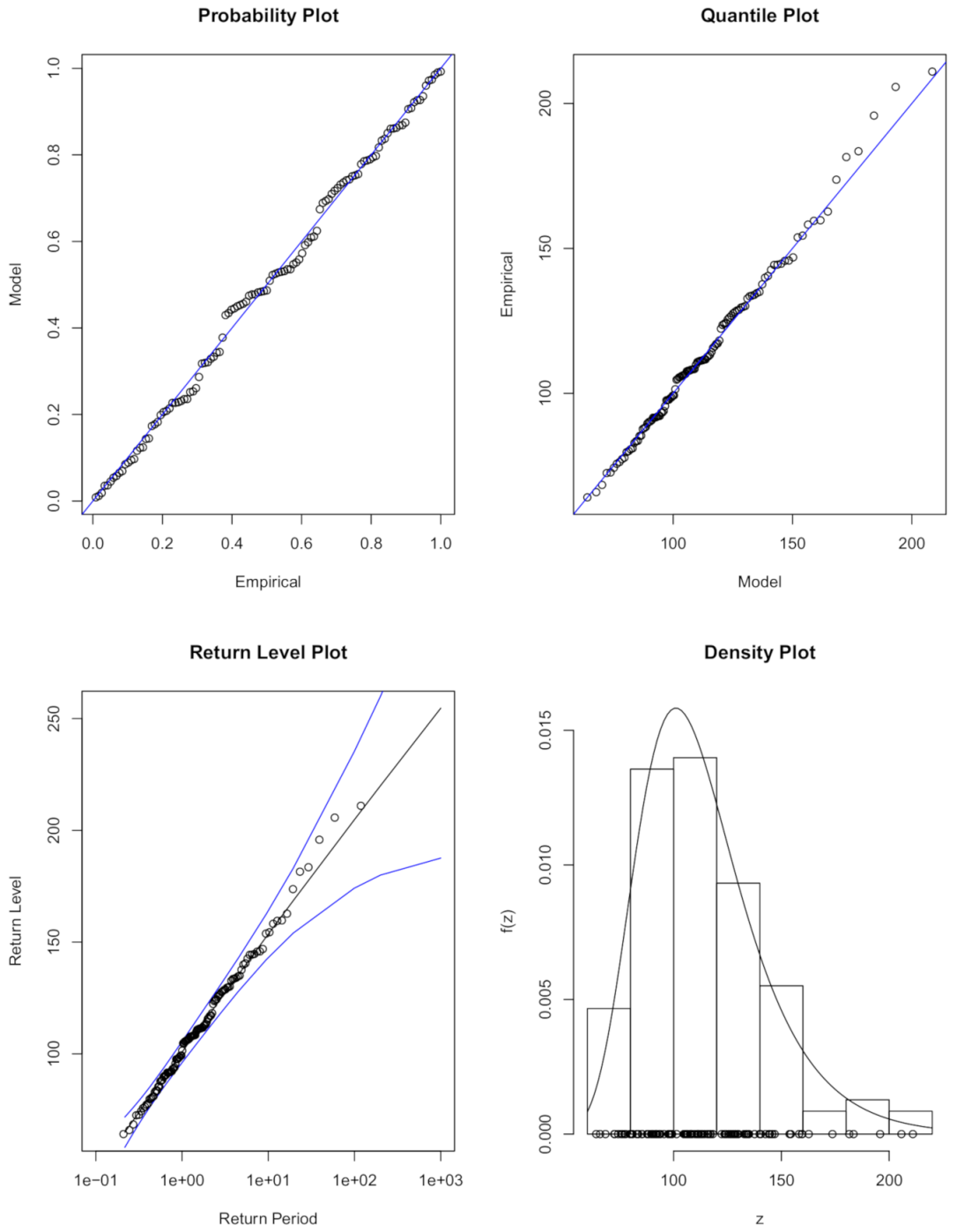
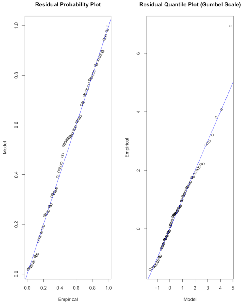
The shape parameter (−0.012) for the model, $M_0$, in (28) indicates that the rainfall data for Eastern Cape can be modelled by the Weibull class of distributions since the shape parameter $\xi <0$. The diagnostic plots for the stationary GEVD model in (28) are presented in Figure 3. The diagnostic plot results in Figure 3 show that the stationary GEVD model, $M_0$, is the best fit for the Eastern Cape monthly rainfall data.

Goodness-of-fit test for Eastern Cape GEVD model

The goodness-of-fit test based on Kolmogorov-Smirnov (K-S) and Anderson-Darling (A-D) tests were performed in order to check if the maximum monthly rainfall data for Eastern Cape follow a stationary GEVD model.

Table 6. Goodness-of-fit for Eastern Cape (1900–2017).

Test	Test Statistic	p-Value
K-S	0.056844	0.8403205
A-D	0.1935343	0.8918115

presents the results of the K-S and A-D goodness-of-fit tests for the selected stationary GEVD model for Eastern Cape.

The hypotheses are formulated as follows

H${}_{\mathbf{0}}$: The monthly rainfall data follow a specified distribution, and

H${}_{\mathbf{1}}$: The monthly rainfall data do not follow the specified distribution.

Since the p-values for both the K-S and A-D tests are greater than the 5% level of significance, $\alpha$ = 0.05, we conclude that the maximum monthly rainfall for Eastern Cape follow the specified stationary GEVD.

4.2.2. Gauteng

The model pairs ($M_0,M_1$) and ($M_0,M_2$) from

Table 7. Non-stationary GEVD models for Gauteng for the period 1900–2017.

Model	$\widehat{{\mathit{\mu }}_0}$	$\widehat{{\mathit{\mu }}_1}$	$\widehat{{\mathit{\mu }}_2}$	$\widehat{{\mathit{\sigma }}_0}$	$\widehat{{\mathit{\sigma }}_1}$	$\widehat{{\mathit{\sigma }}_2}$	$\widehat{\mathit{\xi }}$	NLLH
$M_0$	141.929	0	0	34.705	0	0	0.117	612.516
$M_1$	142.629	−0.012	0	34.669	0	0	0.118	612.505
$M_2$	141.690	0	0	32.345	0.032	0	0.128	612.391
$M_3$	140.811	0.015	0	32.138	0.039	0	0.129	612.380
$M_4$	141.474	0.016	0.000	32.514	0.0319	0	0.133	612.389
$M_5$	142.238	−0.002	0	39.864	−0.303	−0.003	0.108	611.664
$M_6$	141.590	0.007	0.000	39.640	−0.300	0.003	0.105	611.663
$M_7$	142.800	0.007	0.000	34.573	0	0	0.125	612.451
$M_8$	142.117	0	0	39.789	−0.302	0.003	0.108	611.661

Key: NLLH = negative log-likelihood.

have the same critical value of ${\chi }_1^2\left(0.05\right)=3.841$ with the deviance statistic values of 0.022 and 0.250 for $M_1$ and $M_2$, respectively. Since the values of the deviance statistics for $M_1$ (0.022) and $M_2$ (0.250) are smaller than the critical value of 3.841, we conclude that both models do not provide any improvement in fit over the stationary GEVD model.

From Table 7, the deviance statistics of model pairs $(M_0,M_3)$ and $(M_0,M_7)$ are 0.272 and 0.130, respectively. Since the values of the deviance statistics for both model pairs are smaller than ${\chi }_2^2\left(0.05\right)=5.991$, it implies that both models do not provide any improvement in fit over the stationary GEVD model. The model pair $(M_0,M_6)$ from Table 7 has ${\chi }_4^2\left(0.05\right)=9.488$ and a deviance statistic value of 1.706. Since the deviance statistic value (1.706) is smaller than the critical value of 9.488, we conclude that model $M_6$ does not provide any improvement in fit over the stationary GEVD model.

The other pairs from Table 7, i.e., $(M_0,M_4)$ and $(M_0,M_5)$, have deviance statistics of 0.254 and 1.704, respectively. These results revealed that model $M_4$, which allows for nonlinear quadratic trend in the location parameter and a linear trend in the scale parameter, does not improve on the stationary GEVD model since the value of the deviance statistic (1.864) is small as compared to the value of ${\chi }_3^2\left(0.05\right)=7.815$. Also, model $M_5$, which allows for linear trend in the location parameter and a nonlinear quadratic trend in the scale parameter, does not provide any improvement on the stationary GEVD model because the value of the deviance statistic is smaller than the critical value of ${\chi }_3^2\left(0.05\right)=7.815$. The model pair $(M_0,M_8)$, which allows for nonlinear quadratic trend in scale parameter with no variation in location parameter, has a deviance statistic of 1.710, which is small compared to the critical value of 5.991 with 2 degrees of freedom. Thus, allowing for a quadratic trend in the scale parameter with no variation in the location parameter does not improve on the stationary GEVD model. Therefore, model $M_8$ is also not worthwhile.

The best fit model for Gauteng is the stationary GEVD model, $M_0$, and is given by

$$GEVD(x,\mu ,\sigma ,\xi )=exp-{\left[1+0.117\left(\frac{x-141.292}{34.705}\right)\right]}^{\frac{-1}{0.117}}.$$

(29)

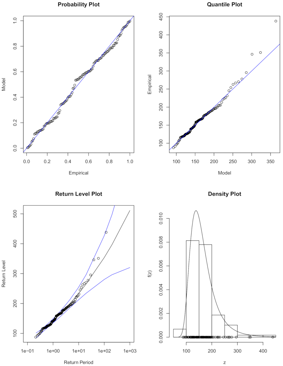
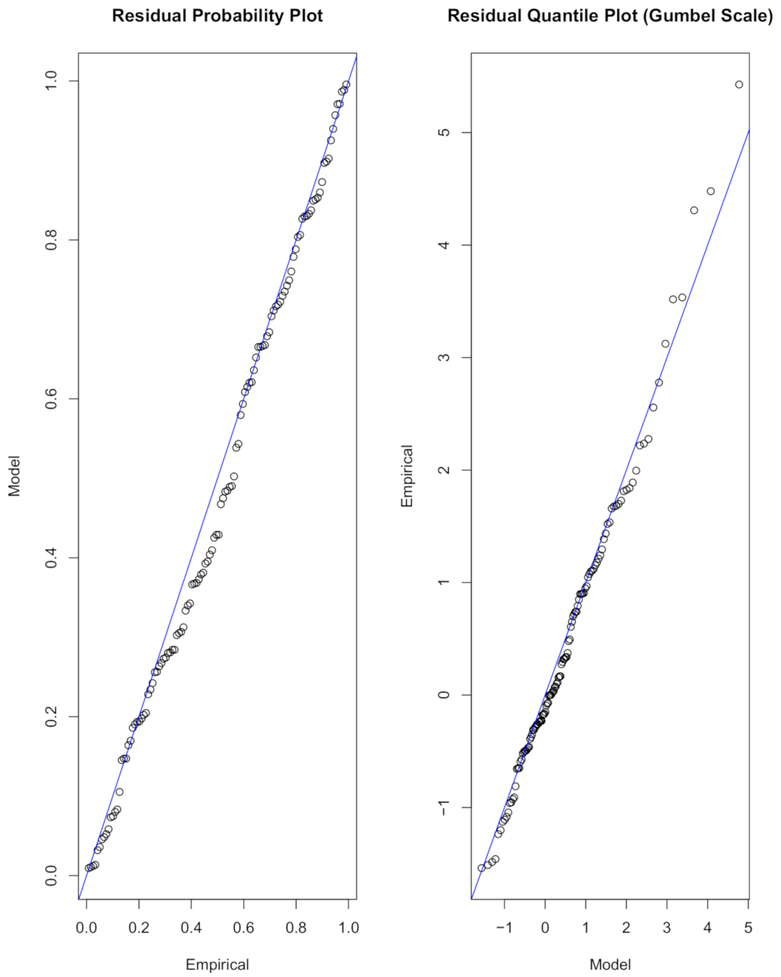
The shape parameter (0.117) for the stationary GEVD model, $M_0$, in (29) indicates that the rainfall data for Gauteng can be modelled using Fréchet distribution class since the shape parameter $\xi >0$. The diagnostic plots for the stationary GEVD model in (29) are presented in Figure 4. The diagnostic plot results in Figure 4 reveal that the stationary GEVD model, $M_0$, in the Fréchet domain of attraction is the best fit for Gauteng monthly rainfall data.

Goodness-of-fit test for Gauteng GEVD model

Kolmogorov-Smirnov (K-S) and Anderson-Darling (A-D) tests were used to determine whether maximum monthly rainfall data for Gauteng follow a stationary GEVD.

Table 8. Goodness-of-fit for Gauteng (1900–2017).

Test	Test Statistic	p-Value
K-S	0.0673058	0.6590246
A-D	0.3562733	0.4519496

presents the results of the K-S and A-D goodness-of-fit tests for Gauteng stationary GEVD model.

The results from Table 8 show that the p-values for both the K-S and A-D tests are not significant (p > 0.05). Therefore, we conclude that the maximum monthly rainfall for Gauteng province follow the specified stationary GEVD.

4.2.3. KwaZulu-Natal

Consider the model pairs ($M_0,M_1$) and ($M_0,M_2$) from

Table 9. Non-stationary GEVD models for KwaZulu-Natal for the period 1900–2017.

Model	$\widehat{{\mathit{\mu }}_0}$	$\widehat{{\mathit{\mu }}_1}$	$\widehat{{\mathit{\mu }}_2}$	$\widehat{{\mathit{\sigma }}_0}$	$\widehat{{\mathit{\sigma }}_1}$	$\widehat{{\mathit{\sigma }}_2}$	$\widehat{\mathit{\xi }}$	NLLH
$M_0$	153.756	0	0	39.560	0	0	0.070	624.418
$M_1$	156.383	−0.044	0	39.518	0	0	0.070	624.313
$M_2$	153.791	0	0	38.808	0.012	0	0.071	624.405
$M_3$	156.817	−0.051	0	40.195	−0.011	0	0.070	624.306
$M_4$	158.193	−0.002	−0.0007	41.398	−0.003	0	0.009	624.106
$M_5$	157.029	−0.006	0	40.021	0.002	−0.0001	0.007	624.305
$M_6$	157.126	−0.005	−0.0008	39.892	0.036	−0.0006	0.098	624.119
$M_7$	146.685	0.464	−0.004	39.308	0	0	0.066	623.294
$M_8$	153.260	0	0	38.741	0.005	0.0000	0.011	624.506

Key: NLLH = negative log-likelihood.

. The critical value for both pairs is ${\chi }_1^2\left(0.05\right)=3.841$ with respective deviance statistic values of 0.210 and 0.026 for the two model pairs. The pairs ($M_0,M_1$) and ($M_0,M_2$) do not provide any improvement in fit over the stationary GEVD model since the deviance statistic values, 0.210 and 0.026, are smaller than the critical value of 3.841 with 1 degree of freedom.

Consider the model pair ($M_0,M_3$) from Table 9 with ${\chi }_2^2\left(0.05\right)=5.991$ and deviance statistic of 0.224 which is too small compared to the critical value of 5.991 with 2 degrees of freedom. Thus, allowing for linear trend in the location and scale parameter is not worthwhile over the stationary GEVD model. The other pairs from Table 9$(M_0,M_4)$ and $(M_0,M_5)$ have deviance statistics of 0.624 and 0.226, respectively. These results revealed that model $M_4$, which allows for nonlinear quadratic trend in the location parameter and a linear trend in the scale parameter, is not worthwhile over the stationary GEVD model since the value of the deviance statistic (0.624) is very small compared to the critical value of ${\chi }_3^2\left(0.05\right)=7.815$. Also, model $M_5$, which allows for linear trend in the location parameter and a nonlinear quadratic trend in the scale parameter, does not provide any improvement in fit over the stationary GEVD model since the value of the deviance statistic (0.226) is too small compared to the value of 7.815 with 3 degrees of freedom.

The model pairs $(M_0,M_7)$ and $(M_0,M_8)$ in Table 9 share a critical value of ${\chi }_2^2\left(0.05\right)=5.991$ with deviance statistic values of 2.248 and −0.176 for $M_7$ and $M_8$, respectively. Since the values of the deviance statistics are smaller than the critical value of 5.991 with 2 degrees of freedom, it implies that both models do not provide any improvement in fit over the stationary GEVD model.

The model pair $(M_0,M_6)$, which allows for nonlinear quadratic trend in both the location and scale parameters in Table 9, has a deviance statistic of 0.598 which is too small compared to the critical value of 9.488 with 4 degrees of freedom. Thus, allowing for a quadratic trend in both the location and scale parameters does not improve on the stationary GEVD model.

Overall, the final best model for KwaZulu-Natal is the stationary GEVD model, $M_0$. The general model for KwaZulu-Natal is given by

$$GEVD(x,\mu ,\sigma ,\xi )=\left\{\begin{array}{c}exp-{\left[1+0.070\left(\frac{x-153.756}{39.560}\right)\right]}^{\frac{-1}{0.070}}.\hfill \end{array}\right.$$

(30)

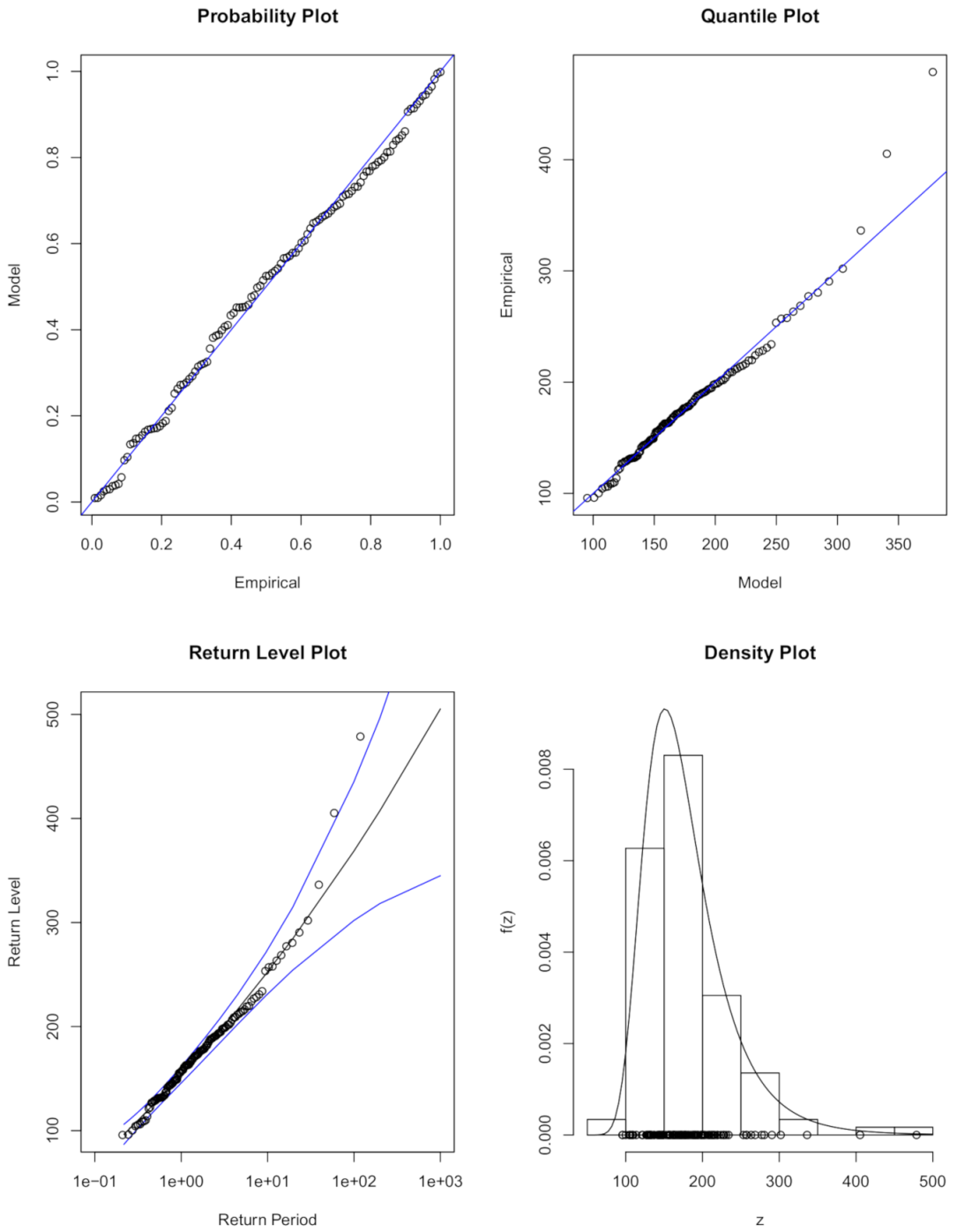
The shape parameter (0.070) for the model $M_0$, in (30) suggests that the rainfall data for KwaZulu-Natal can be modelled using Fréchet class of distributions since the shape parameter $\xi >0$. The diagnostic plots for the stationary GEVD model in (30) are presented in Figure 5. The results in Figure 5 show that the stationary GEVD model, $M_0$, is the best fit for KwaZulu-Natal maximum monthly rainfall data since all the four diagnostic plots suggest a reasonable good fit.

Goodness-of-fit test for KwaZulu-Natal GEVD model

Kolmogorov-Smirnov (K-S) and Anderson-Darling (A-D) tests were used to determine whether maximum monthly rainfall data for KwaZulu-Natal follow a stationary GEVD model.

Table 10. Goodness-of-fit for KwaZulu-Natal (1900–2017).

Test	Test Statistic	p-Value
K-S	0.04470146	0.9724252
A-D	0.3284819	0.5135279

presents the K-S and A-D goodness-of-fit tests results for KwaZulu-Natal GEVD.

From Table 10, the p-values for both K-S and A-D tests are insignificant (p > 0.05) at 5% level of significance. Thus, we conclude that the maximum monthly rainfall for KwaZulu-Natal follow the specified stationary GEVD model.

4.2.4. Limpopo

The stationary GEVD model for Limpopo data (i.e., model $M_0$) has a maximum NLLH of 669.707. A GEVD model with linear trend in the location parameter (i.e., $M_1$) has a maximum NLLH of 666.705 (see

Table 11. Non-stationary GEVD models for Limpopo for the period 1904–2017.

Model	$\widehat{{\mathit{\mu }}_0}$	$\widehat{{\mathit{\mu }}_1}$	$\widehat{{\mathit{\mu }}_2}$	$\widehat{{\mathit{\sigma }}_0}$	$\widehat{{\mathit{\sigma }}_1}$	$\widehat{{\mathit{\sigma }}_2}$	$\widehat{\mathit{\xi }}$	NLLH
$M_0$	132.224	0	0	65.611	0	0	−0.097	669.707
$M_1$	105.813	0.423	0	61.752	0	0	−0.067	666.705
$M_2$	133.060	0	0	78.463	−0.289	0	−0.030	665.327
$M_3$	115.204	0.258	0	73.135	−0.218	0	−0.036	664.200
$M_4$	74.261	2.073	−0.015	65.293	−0.178	0	0.040	660.187
$M_5$	122.793	0.132	0	105.672	−1.988	0.014	0.105	655.757
$M_6$	107.754	0.732	−0.005	99.611	−1.756	0.013	0.094	655.184
$M_7$	62.447	2.432	−0.017	54.826	0	0	0.047	661.797
$M_8$	133.880	0	0	107.223	−2.009	0.015	0.008	665.038

Key: NLLH = negative log-likelihood.

). The deviance statistic for comparing these two models is therefore D = 2(669.707 − 666.705) = 6.004, which is greater than the critical value of 3.841 with 1 degree of freedom. Therefore, model $M_1$ provides an improvement in fit over the stationary GEVD model. The likelihood ratio test for ${\mu }_1$ = 0 has p-value = 0.005, which is significant at 5% level of significance (p < 0.05). This clearly shows that the non-stationary GEVD model is worthwhile and provides an improvement in fit over the stationary GEVD model.

Consider the pair of models $(M_0,M_2)$ from Table 11. The deviance statistic is 2(669.707 − 665.327) = 8.760, which is large compared to ${\chi }_1^2\left(0.05\right)=3.841$. Thus, allowing for a linear trend in the scale parameter improves on the stationary GEVD model. The likelihood ratio test for ${\sigma }_1$ = 0 has p-value of 0.001, implying that the linear trend in the scale parameter is significant at 5% level of significance (p < 0.05). This indicates that model $M_2$ is important and does provide an improvement in fit over the stationary GEVD model.

From Table 11, the pair of models $(M_0,M_3)$, has the deviance statistic of 11.014, which is greater than the critical value of 5.991 with 2 degrees of freedom, implying that model $M_3$ provides an improvement in fit over the stationary GEVD model. The likelihood ratio test for ${\mu }_1$ = 0 has p-value = 0.067, which indicates that the likelihood ratio test is not significant at 5% level of significance (p > 0.05), while the likelihood ratio test for ${\sigma }_1$ = 0 has p-value = 0.013, which suggests that the likelihood ratio test is significant at 5% level of significance (p < 0.05).

The other pairs from Table 11, $(M_0,M_4)$ and $(M_0,M_5)$, have deviance statistic values of 19.040 and 7.900, respectively. These results suggest that model $M_4$, which allows for nonlinear quadratic trend in the location parameter and linear trend in the scale parameter, provides an improvement in fit over the stationary GEVD model since the value of the deviance statistic (19.040) is larger as compared to the value of ${\chi }_3^2\left(0.05\right)=7.815$. The likelihood ratio test for ${\mu }_1$ = 0 has p-value = 0.001, for ${\mu }_2$ = 0 it has p-value of 0.002, and for ${\sigma }_1$ = 0 it has p-value = 0.034, which are all significant at 5% level of significance (p < 0.05). Also, model $M_5$ which allows for linear trend in the location parameter and a nonlinear quadratic trend in the scale parameter, provides an improvement in the stationary GEVD model since the value of the deviance statistic is greater than the value of ${\chi }_3^2\left(0.05\right)=7.815$. The likelihood ratio test for ${\mu }_1$ = 0 has p-value = 0.236, which is not significant at 5% level of significance (p > 0.05), while the likelihood ratio tests for ${\sigma }_1$ = 0, and ${\sigma }_2$ = 0, all have p-values < 0.001, which are both significant at 5% level of significance (p < 0.05).

The model pair $(M_0,M_6)$, which allows for nonlinear quadratic trend in both the location and scale parameters in Table 11, has a deviance statistic of 9.046 which is small compared to the critical value of 9.488 with 4 degrees of freedom. Thus, allowing for a quadratic trend in both the location and scale parameters is not worthwhile in fit over the stationary GEVD model $M_0$. The likelihood ratio test for ${\mu }_1$ = 0 has p-value = 0.145, and for ${\mu }_2$ = 0 has p-value = 0.185, which is insignficant at 5% level of significance (p > 0.05), while the likelihood ratio test for ${\sigma }_1$ = 0, and ${\sigma }_2$ = 0, all have p-values < 0.001, which are both significant at 5% level of significance (p < 0.05).

Consider the model pair $(M_0,M_7)$ in Table 11 with deviance statistic of 15.820, which is greater than the critical value of ${\chi }_2^2\left(0.05\right)=5.991$, indicating that the non-stationary GEVD model provides an improvement in fit over the stationary GEVD model. The likelihood ratio tests for ${\mu }_1$ = 0, and ${\mu }_2$ = 0 have p-values < 0.001, which indicate that the likelihood ratio tests are significant at 5% level of significance (p < 0.05) for the quadratic trend in the location parameter with no variation in the scale parameter. This implies that the non-stationary GEVD model, $M_8$, is worthwhile and does give an improvement in fit over the stationary GEVD model.

Consider the model pair $(M_0,M_8)$ from Table 11 with ${\chi }_2^2\left(0.05\right)=5.991$ and deviance statistic of 9.338. The likelihood ratio tests for ${\sigma }_1$= 0 and ${\sigma }_2$ = 0 have p-values <0.001. These results show that the nonlinear quadratic trend in scale parameter with no variation in the location parameter is significant at 5% level of significance (p < 0.05). The deviance statistic (9.338) is greater than the critical value of 5.991, which implies that the non-stationary GEVD model, $M_8$, is important and does provide an improvement in fit over the stationary GEVD model.

Overall, Limpopo has five competing non-stationary GEVD models: $M_1$, $M_2$, $M_4$, $M_7$ and $M_8$, for which only two models were considered based on their deviance statistic values as main and alternative best models. The best non-stationary GEVD model is $M_4$, which has a nonlinear quadratic trend in the location parameter and a linear trend in the scale parameter, and is given by

$$GEVD(x,\mu ,\sigma ,\xi )=\left\{\begin{array}{c}exp-{\left[1+0.040\left(\frac{x-74.261}{65.293}\right)\right]}^{\frac{-1}{0.040}}.\hfill \end{array}\right.$$

(31)

The alternative non-stationary GEVD model is $M_7$, which has a nonlinear quadratic trend in the location parameter and no variation in the scale parameter, and is given by:

$$GEVD(x,\mu ,\sigma ,\xi )=\left\{\begin{array}{c}exp-{\left[1+0.047\left(\frac{x-62.447}{54.826}\right)\right]}^{\frac{-1}{0.047}}.\hfill \end{array}\right.$$

(32)

The shape parameters in (31) and (32), that is, 0.040 and 0.047 for the models $M_4$ and $M_7$, respectively, are positive, which suggests that the rainfall data for Limpopo can be modelled using the Fréchet distribution class since the shape parameter $\xi >0$. The diagnostic plots for the non-stationary GEVD model in (31) are presented in Figure 6. The results in Figure 6 show that model $M_4$ is the best fit for Limpopo maximum monthly rainfall data since the two diagnostic plots indicate a reasonable good fit for the non-stationary GEVD model with a nonlinear quadratic trend in the location parameter and a linear trend in the scale parameter.

Goodness-of-fit test for Limpopo non-stationary GEVD model

Kolmogorov-Smirnov (K-S) and Anderson-Darling (A-D) tests were used to determine whether maximum monthly rainfall data for Limpopo follows the non-stationary GEVD model, $M_4$.

Table 12. Goodness-of-fit for Limpopo (1904–2017).

Test	Test Statistic	p-Value
K-S	0.07362455	0.5445211
A-D	1.133259	0.005549523

presents the K-S and A-D goodness-of-fit tests.

From Table 12, the p-value for the K-S test is insignificant (p > 0.05), implying that the maximum monthly rainfall for Limpopo follows the non-stationary GEVD model, while the results from the A-D test suggest that the maximum monthly rainfall for Limpopo do not follow the specified non-stationary GEVD model (p < 0.05). This contradiction in the results of the two goodness-of-fit tests may be a cause for concern, and may suggest that the selected non-stationary GEVD model, $M_4$, may not model the extreme right tails of the Limpopo maximum monthly rainfall data quite well.

4.2.5. Mpumalanga

The model pairs $(M_0,M_1)$ and $(M_0,M_2)$ in

Table 13. Non-stationary GEVD models for Mpumalanga for the period 1904–2017.

Model	$\widehat{{\mathit{\mu }}_0}$	$\widehat{{\mathit{\mu }}_1}$	$\widehat{{\mathit{\mu }}_2}$	$\widehat{{\mathit{\sigma }}_0}$	$\widehat{{\mathit{\sigma }}_1}$	$\widehat{{\mathit{\sigma }}_2}$	$\widehat{\mathit{\xi }}$	NLLH
$M_0$	155.612	0	0	59.246	0	0	−0.325	643.234
$M_1$	124.429	0.512	0	54.437	0	0	−0.261	638.230
$M_2$	159.885	0	0	71.217	−0.274	0	−0.228	639.616
$M_3$	131.503	0.428	0	69.312	−0.268	0	−0.240	633.469
$M_4$	114.907	1.296	−0.007	71.758	−0.310	0	−0.207	631.569
$M_5$	161.943	−0.031	0	113.977	−2.386	0.017	−0.006	631.285
$M_6$	145.643	−0.001	0.002	108.921	−2.381	0.017	0.076	630.978
$M_7$	145.591	0.324	−0.0009	58.266	0	0	−0.328	640.037
$M_8$	161.734	0	0	100.364	−1.981	0.014	−0.161	628.659

Key: NLLH = negative log-likelihood.

share the critical value of ${\chi }_1^2\left(0.05\right)=3.841$ with respective deviance statistic values of 10.008 and 7.236. The two pairs have p-values of 0.001 and 0.003 for ${\mu }_1$ = 0 and ${\sigma }_1$ = 0, respectively for model $M_1$ and $M_2$. These results suggest that the model pairs $(M_0,M_1)$ and $(M_0,M_2)$ are significant at 5% level of significance (p < 0.05). The deviance statistic values for the two models are large in comparison to ${\chi }_1^2\left(0.05\right)=3.841$. Thus, we conclude that models $M_1$ and $M_2$ provide a significant improvement over the stationary GEVD model, $M_0$.

From Table 13, the pair of models $(M_0,M_3)$ has a deviance statistic of 19.530, which is greater than the critical value of 5.991 with 2 degrees of freedom, implying that model $M_3$ provides an improvement in fit over the stationary GEVD model. The likelihood ratio tests for ${\mu }_1$ = 0 and ${\sigma }_1$ = 0 have p-values < 0.001, which indicate that the likelihood ratio tests are significant at 5% level of significance (p < 0.05) for both the location and scale parameters, implying that the non-stationary GEVD model, $M_3$, is important and does provide an improvement in fit over the stationary GEVD model.

The other model pairs from Table 13, $(M_0,M_4)$ and $(M_0,M_5)$, have deviance statistic values of 23.330 and 23.898, respectively. These results suggest that model $M_4$, which allows for nonlinear quadratic trend in the location parameter and linear trend in the scale parameter, is worthwhile over the stationary GEVD model since the value of the deviance statistic (23.330) is greater than the critical value of ${\chi }_3^2\left(0.05\right)=7.815$. The likelihood ratio test for ${\mu }_1$ = 0 has p-value= 0.392, and for ${\mu }_2$ = 0 it has p-value of 0.096, which are both not significant at 5% level of significance (p > 0.05), but the likelihood ratio test for ${\sigma }_1$ = 0 has p-value < 0.001, which is significant at 5% level of significance (p < 0.05). On the other hand, model $M_5$ which allows for linear trend in the location parameter and a nonlinear quadratic trend in the scale parameter, provides an improvement in fit over the stationary GEVD model since the value of the deviance statistic is greater than the value of ${\chi }_3^2\left(0.05\right)=7.815$. The likelihood ratio test for ${\mu }_1$ = 0, ${\sigma }_1$ = 0 and ${\sigma }_2$ = 0, all have p-values < 0.001, which are significant at 5% level of significance (p < 0.05).

The model pair $(M_0,M_6)$ in Table 13, which allows for nonlinear quadratic trend in both the location and scale parameters, has a deviance statistic of 24.512 which is greater than the critical value of 9.488 with 4 degrees of freedom. Thus, allowing for a quadratic trend in both location and the scale parameters is worthwhile in fit over the stationary GEVD model, $M_0$. The likelihood ratio test for ${\mu }_1$= 0 has p-value = 0.499, and ${\mu }_2$ = 0 has p-value = 0.303, which is insignificant at 5% level of significance (p > 0.05), while the likelihood ratio tests for ${\sigma }_1$ = 0 and ${\sigma }_2$ = 0 all have p-values < 0.001, which are significant at 5% level of significance (p < 0.05).

Consider the model pair $(M_0,M_7)$ in Table 13, with a deviance statistic of 6.394 which is greater than the critical value of ${\chi }_2^2\left(0.05\right)=5.991$. These results show that the non-stationary GEVD model provides an improvement in fit over the stationary GEVD model. The likelihood ratio test for ${\mu }_1$ = 0 has p-value = 0.369 and for ${\mu }_2$ = 0 it has p-value = 0.449, which are both not significant at 5% level of significance (p > 0.05). This implies that model $M_7$, with a quadratic trend in the scale parameter and no variation in the location parameter is not worthwhile over the stationary GEVD model.

Consider the model pair $(M_0,M_8)$ from Table 13 with ${\chi }_2^2\left(0.05\right)=5.991$ and deviance statistic value of 29.150. The likelihood ratio tests for ${\sigma }_1$= 0 and ${\sigma }_2$ = 0 have p-values <0.001. These results show that the nonlinear quadratic trend in scale parameter with no variation in the location parameter is significant at 5% level of significance (p < 0.05). The deviance statistic (29.150) is greater than the critical value of 5.991, which implies that the non-stationary GEVD model, $M_8$, is important and does provides an improvement in fit over the stationary GEVD model.

In general, Mpumalanga has five competing non-stationary GEVD models: $M_1$, $M_2$, $M_3$, $M_5$ and $M_8$, for which only two models were considered based on their deviance statistic values as main and alternative best models. The best non-stationary GEVD model is $M_8$, which has a nonlinear quadratic trend in the scale parameter and no variation in the location parameter, and is given by

$$GEVD(x,\mu ,\sigma ,\xi )=\left\{\begin{array}{c}exp-{\left[1-0.161\left(\frac{x-161.734}{100.364}\right)\right]}^{\frac{1}{0.161}}.\hfill \end{array}\right.$$

(33)

The alternative non-stationary GEVD model, is $M_5$, which has a linear trend in location parameter and nonlinear quadratic trend in scale parameter and is given by:

$$GEVD(x,\mu ,\sigma ,\xi )=\left\{\begin{array}{c}exp-{\left[1-0.006\left(\frac{x-161.943}{113.977}\right)\right]}^{\frac{1}{0.006}}.\hfill \end{array}\right.$$

(34)

The shape parameters in (33) and (34), that is, −0.161 and −0.006 for the respective models $M_8$ and $M_5$ are negative, which indicate that the rainfall data for Mpumalanga can be modelled using Weibull distribution class since the shape parameter $\xi <0$. The diagnostic plots for the non-stationary GEVD model in (33) are presented in Figure 7. The results in Figure 7 show that the non-stationary GEVD model, $M_8$, is the best fit for Mpumalanga maximum monthly rainfall data since the two diagnostic plots suggest a reasonable good fit for the non-stationary GEVD model with a quadratic trend in the scale parameter and no variation in other parameters.

Goodness-of-fit test for Mpumalanga non-stationary GEVD model

Kolmogorov-Smirnov (K-S) and Anderson-Darling (A-D) tests were used to determine whether maximum monthly rainfall data for Mpumalanga follow the non-stationary GEVD model, $M_8$.

Table 14. Goodness-of-fit for Mpumalanga (1904–2017).

Test	Test Statistic	p-Value
K-S	0.08991587	0.2957988
A-D	1.791518	0.0001310069

presents the K-S and A-D goodness-of-fit test results for Mpumalanga non-stationary GEVD model, $M_8$.

From Table 14, the p-value for the K-S test is insignificant (p > 0.05), implying that the maximum monthly rainfall for Mpumalanga follows the specified non-stationary GEVD model. On the other hand, the results from the A-D test contradict the results from the K-S test. The explanation for this contradiction is similar to that given for the Limpopo province best model.

5. Conclusions

In this paper, stationarity test, which included the augmented Dickey-Fuller (ADF), Phillips-Perron (PP) and Kwiatkowski-Phillips-Schmidt-Shin (KPSS) tests, was done. The findings from the KPSS test suggest that monthly rainfall data for all the five provinces are not stationary, while the findings from the PP test contradict those from KPSS test. On the other hand, the findings for the ADF stationarity test for Eastern Cape, Limpopo and Mpumalanga suggest that the monthly rainfall data are stationary, which is a further contradiction to the KPSS findings. However, ADF stationarity test findings for Gauteng and KwaZulu-Natal provinces concur with those from KPSS test. The study also employed Jarque-Bera (JB), Shapiro–Wilk (SW) and chi-square test methods to check whether the monthly rainfall data were normally distributed. Findings from the JB, SW and chi-square normality tests revealed that the monthly rainfall data for all the five provinces do not come from a normal distribution.

The study analysed the long-term trends of monthly rainfall data in the five selected provinces of South Africa from 1900 to 2017. Two trend analysis techniques were applied in this study, the Mann-Kendall test and Sen’s slope. Findings from the Mann-Kendall test revealed statistically significant monotonic decreasing trends in Eastern Cape, Gauteng and Kwazulu-Natal provinces, while in Limpopo and Mpumalanga provinces the trends were also revealed to be monotonically decreasing, but insignificant. The Mann-Kendall test statistic findings for Eastern Cape, Gauteng, KwaZulu-Natal and Limpopo were in agreement with the findings from Sen’s slope estimator method. However, the Mann-Kendall test findings for Mpumalanga slightly differed from Sen’s slope estimator findings. This slight difference can be interpreted as a confirmation of the insignificance of long-term trend and slope for Mpumalanga monthly rainfall.

The study further analysed and discussed in detail the modelling of monthly rainfall extremes using the non-stationary GEVD approach which belongs to the block maxima realisation [40]. The maximum likelihood estimation method was used to obtain the estimates of the parameters. The stationary GEVD was found as the best distribution model for Eastern Cape, Gauteng and KwaZulu-Natal provinces. Furthermore, model fitting supported non-stationary GEVD models for Limpopo and Mpumalanga maximum monthly rainfall, with nonlinear quadratic trend in the location parameter and a linear trend in the scale parameter for Limpopo, while for Mpumalanga the non-stationary GEVD model with a nonlinear quadratic trend in the scale parameter and no variation in the location parameter fitted well to the maximum monthly rainfall data. The study further revealed that the maximum monthly rainfall for Eastern Cape and Mpumalanga can be modelled by distributions in the negative-Weibull domain, while maximum monthly rainfall data for Gauteng, KwaZulu-Natal and Limpopo follow distributions in the Fréchet distribution class.

Model diagnostics, which included the Kolmogorov-Smirnov (K-S) and Anderson-Darling (A-D) tests among others, further confirmed that the maximum monthly rainfall for Eastern Cape, Gauteng and KwaZulu-Natal follow the stationary GEVD, while for Limpopo and Mpumalanga the K-S findings showed that the maximum monthly rainfall for these two provinces follow the non-stationary GEVD model. The latter findings could not be confirmed by the A-D goodness-of-fit test.

Findings from this study can help us with information necessary for decision makers to establish strategies for proper planning of agriculture, infrastructure, drainage system and other water resource applications in South Africa. These findings may also assist South African government agencies to improve the socio-economic conditions of the country under the changing rainfall patterns and impending global warming.

This study will form a benchmark for monthly rainfall studies of this kind in these provinces of South Africa. Further studies may look to extend this study into spatial extremes, copula and conditional extremes modelling, as well as Bayesian extreme value modelling approaches.

References

1. Lakhraj-Govender, R.; Grab, S.W. Rainfall and river flow trends for the Western Cape Province, South Africa. S. Afr. J. Sci. 2019, 115, 1–6. [Google Scholar] [CrossRef]
2. Masereka, E.M.; Ochieng, G.M.; Snyman, J. Statistical analysis of annual maximum daily rainfall for Nelspruit and its environs. Jàmbá J. Disaster Risk Stud. 2018, 10, 1–10. [Google Scholar] [CrossRef] [PubMed] [Green Version]
3. Chu, P.S.; Zhao, X.; Ruan, Y.; Grubbs, M. Extreme rainfall events in the Hawaiian Islands. J. Appl. Meteorol. Climatol. 2009, 48, 502–516. [Google Scholar] [CrossRef] [Green Version]
4. Muchuru, S.; Landman, W.A.; DeWitt, D.; Lötter, D. Seasonal rainfall predictability over the Lake Kariba catchment area. Water SA 2014, 40, 461–470. [Google Scholar] [CrossRef] [Green Version]
5. Syafrina, A.H.; Zalina, M.D.; Juneng, L. Historical trend of hourly extreme rainfall in Peninsular Malaysia. Theor. Appl. Climatol. 2015, 120, 259–285. [Google Scholar] [CrossRef] [Green Version]
6. Mzezewa, J.; Misi, T.; Van Rensburg, L. Characterisation of rainfall at a semi-arid ecotope in the Limpopo Province (South Africa) and its implications for sustainable crop production. Water SA 2010, 36, 19–26. [Google Scholar] [CrossRef] [Green Version]
7. Manhique, A.J.; Reason, C.J.C.; Silinto, B.; Zucula, J.; Raiva, I.; Congolo, F.; Mavume, A.F. Extreme rainfall and floods in Southern Africa in January 2013 and associated circulation patterns. Nat. Hazards 2015, 77, 679–691. [Google Scholar] [CrossRef]
8. Du Plessis, J.A.; Schloms, B. An investigation into the evidence of seasonal rainfall pattern shifts in the Western Cape, South Africa. J. S. Afr. Inst. Civ. Eng. 2017, 59, 47–55. [Google Scholar] [CrossRef] [Green Version]
9. Nash, D.J.; Pribyl, K.; Klein, J.; Neukom, R.; Endfield, G.H.; Adamson, G.C.; Kniveton, D.R. Seasonal rainfall variability in Southeast Africa during the nineteenth century reconstructed from documentary sources. Clim. Chang. 2016, 134, 605–619. [Google Scholar] [CrossRef]
10. Dyson, L.L. Heavy daily-rainfall characteristics over the Gauteng Province. Water SA 2009, 35, 627–638. [Google Scholar] [CrossRef] [Green Version]
11. Nel, W. Rainfall trends in the KwaZulu-Natal Drakensberg region of South Africa during the twentieth century. Int. J. Climatol. J. R. Meteorol. Soc. 2009, 29, 1634–1641. [Google Scholar] [CrossRef]
12. Thomas, D.S.; Twyman, C.; Osbahr, H.; Hewitson, B. Adaptation to climate change and variability: Farmer responses to intra-seasonal precipitation trends in South Africa. In African Climate and Climate Change; Charles, J.R.W., Dominic, R., Eds.; Springer: Dordrecht, South Africa, 2011; Volume 83, pp. 155–178. [Google Scholar]
13. Pindura, T.H. An Assessment of Water Security and Hydrology Resources in the Face of Climate Variability: The Case Study of Nkonkobe Local Municipality, Eastern Cape. South Africa. Ph.D. Thesis, University of Fort Hare, Alice, South Africa, 2016. [Google Scholar]
14. Oduniyi, O.S. Climate Change Awareness: A Case Study of Small Scale Maize Farmers in Mpumalanga Province, South Africa. Ph.D. Thesis, University of South Africa, Pretoria, South Africa, 2013. [Google Scholar]
15. Holloway, A.J.; Fortune, G.; Chasi, V.; Beckman, T.; Pharoah, R.; Poolman, E.; Punt, C.; Zweig, P.; RADAR Western Cape 2010: Risk and Development Annual Review. Technical Report; In Disaster Mitigation for Sustainable Livelihoods Programme (DiMP); 2010. Available online: https://www.preventionweb.net/organizations/64 (accessed on 14 January 2021).
16. Fedorová, D. Selection of unit root test on the basis of length of the time series and value of ar (1) parameter. Statistika 2016, 96, 47–64. [Google Scholar]
17. Paparoditis, E.; Politis, D.N. The asymptotic size and power of the augmented Dickey-Fuller test for a unit root. Econom. Rev. 2018, 37, 955–973. [Google Scholar] [CrossRef] [Green Version]
18. Liolios, E. Google Trends as a predictive tool for the sales of the Apple. Master’s Thesis, International Hellenic University, 2015. [Google Scholar]
19. Phillips, P.C.; Perron, P. Testing for a unit root in time series regression. Biometrika 1998, 75, 335–346. [Google Scholar] [CrossRef]
20. Kwiatkowski, D.; Phillips, P.C.B.; Schmidt, P.; Shin, Y. Testing the null hypothesis of stationarity against the alternative of a unit root: How sure are we that economic time series have a unit root? J. Econom. 1992, 54, 159–178. [Google Scholar] [CrossRef]
21. Shi, Q.; Li, B.; Alexiadis, S. Testing the real interest parity hypothesis in six developed countries. Int. Res. J. Financ. Econ. 2012, 86, 168–180. [Google Scholar]
22. Wi, S.; Valdés, J.B.; Steinschneider, S.; Kim, T.W. Non-stationary frequency analysis of extreme precipitation in South Korea using peaks-over-threshold and annual maxima. Stoch. Environ. Res. Risk Assess. 2016, 30, 583–606. [Google Scholar] [CrossRef]
23. Da Silva, R.M.; Santos, C.A.; Moreira, M.; Corte-Real, J.; Silva, V.C.; Medeiros, I.C. Rainfall and river flow trends using Mann–Kendall and Sen’s slope estimator statistical tests in the Cobres River basin. Nat. Hazards 2015, 77, 1205–1221. [Google Scholar] [CrossRef]
24. Sen, P.K. Estimates of the regression coefficients based on Kendall’s tau. J. Am. Stat. Assoc. 1968, 63, 1379–1389. [Google Scholar] [CrossRef]
25. Partal, T.; Kahya, E. Trend analysis in Turkish precipitation data. Hydrol. Process. Int. J. 2006, 20, 2011–2026. [Google Scholar] [CrossRef]
26. Ali, R.O.; Abubaker, S.R. Trend analysis using Mann-Kendall, Sen’s slope estimator test and innovative trend analysis method in Yangtze River basin, China. Int. J. Eng. Technol. 2019, 8, 110–119. [Google Scholar]
27. Adefisoye, J.; Kibria, B.M.G.; George, F. Performances of several univariate tests of normality: An empirical study. J. Biom. Biostat. 2016, 7, 1–8. [Google Scholar]
28. Das, K.R.; Imon, A.H.M.R. A brief review of tests for normality. Am. J. Theor. Appl. Stat. 2016, 5, 5–12. [Google Scholar]
29. Ferreira, A.; de Haan, L. On the block maxima method in extreme value theory: PWM estimators. Ann. Stat. 2015, 43, 276–298. [Google Scholar] [CrossRef] [Green Version]
30. Syafrina, A.H.; Norzaida, A.; Ain, J.J. Stationary and Nonstationary Generalized Extreme Value Models for Monthly Maximum Rainfall in Sabah. J. Phys. Conf. Ser. 2019, 1366, 1–6. [Google Scholar] [CrossRef]
31. Ngailo, T.; Shaban, N.; Reuder, J.; Rutalebwa, E.; Mugume, I. Non homogeneous poisson process modelling of seasonal extreme rainfall events in Tanzania. Int. J. Sci. Res. 2016, 5, 1858–1868. [Google Scholar]
32. Coles, S.; Bawa, J.; Trenner, L.; Dorazio, P. An Introduction to Statistical Modeling of Extreme Values; Springer: London, UK, 2001; Volume 208. [Google Scholar]
33. Hundecha, Y.; St-Hilaire, A.; Ouarda, T.B.M.J.; El Adlouni, S.; Gachon, P.A. Nonstationary extreme value analysis for the assessment of changes in extreme annual wind speed over the Gulf of St. Lawrence, Canada. J. Appl. Meteorol. Climatol. 2008, 47, 2745–2759. [Google Scholar] [CrossRef]
34. Panagoulia, D.; Economou, P.; Caroni, C. Stationary and nonstationary generalized extreme value modelling of extreme precipitation over a mountainous area under climate change. Environmetrics 2014, 25, 29–43. [Google Scholar] [CrossRef]
35. Alam, M.A.; Emura, K.; Farnham, C.; Yuan, J. Best-fit probability distributions and return periods for maximum monthly rainfall in Bangladesh. Climate 2018, 6, 9. [Google Scholar] [CrossRef] [Green Version]
36. Chikobvu, D.; Chifurira, R. Modelling of extreme minimum rainfall using generalised extreme value distribution for Zimbabwe. S. Afr. J. Sci. 2015, 111, 1–8. [Google Scholar] [CrossRef] [Green Version]
37. Sharma, M.A.; Singh, J.B. Use of probability distribution in rainfall analysis. N. Y. Sci. J. 2015, 3, 40–49. [Google Scholar]
38. Iyamuremye, E.; Mung’atu, J.; Mwita, P. Extreme Value Modelling of Rainfall Using Poisson-generalized Pareto Distribution: A Case Study Tanzania. Int. J. Stat. Distrib. Appl. 2019, 5, 67–75. [Google Scholar] [CrossRef] [Green Version]
39. Osman, Y.Z.; Fealy, R.; Sweeney, J.C. Modelling extreme temperatures in Ireland under global warming using a hybrid peak–over–threshold and generalised Pareto distribution approach. Int. J. Glob. Warm. 2015, 7, 21–47. [Google Scholar] [CrossRef] [Green Version]
40. Maposa, D.; Cochran, J.J.; Lesaoana, M. Modelling non-stationary annual maximum flood heights in the lower Limpopo River basin of Mozambique. Jàmbá J. Disaster Risk Stud. 2016, 8, a185. [Google Scholar] [CrossRef]
Figure 1. Time series plot for monthly rainfall in (a) Eastern Cape 1900–2017, (b) Gauteng 1900–2017, (c) KwaZulu-Natal 1900–2017, (d) Limpopo 1904–2017 and (e) Mpumalanga 1904–2017.
Hydrology 08 00070 g001
Figure 2. Time series plot of the annual block maximum rainfall observed in (a) Eastern Cape 1900–2017, (b) Gauteng 1900–2017, (c) KwaZulu-Natal 1900–2017, (d) Limpopo 1904–2017 and (e) Mpumalanga 1904–2017.
Hydrology 08 00070 g002
Figure 3. Diagnostic plots for the stationary GEVD best fitting model for Eastern Cape province.
Hydrology 08 00070 g003
Figure 4. Diagnostic plots for the stationary GEVD best fitting model for Gauteng province.
Hydrology 08 00070 g004
Figure 5. Diagnostic plots for the stationary GEVD best fitting model for KwaZulu-Natal province.
Hydrology 08 00070 g005
Figure 6. Diagnostic plots for the non-stationary GEVD best fitting model for Limpopo province.
Hydrology 08 00070 g006
Figure 7. Diagnostic plots for the non-stationary GEVD best fitting model for Mpumalanga province.
Hydrology 08 00070 g007