A Spatially Distributed, Physically-Based Modeling Approach for Estimating Agricultural Nitrate Leaching to Groundwater

Abstract

Nitrogen-nitrate, while being fundamental for crop production, is of particular concern in the agricultural sector, as it can easily leach to the water table, worsening groundwater quality. Numerical models and Geographic Information System may support the estimation of nitrate leaching rates in space and time, to support sustainable agricultural management practices. In this paper, we present a module for the simulation of the processes involved in the nitrogen cycle in the unsaturated zone, including nitrate leaching. This module was developed taking steps from the ANIMO and EPIC model frameworks and coupled to the hydrological models integrated within the FREEWAT platform. As such, the nitrogen cycle module was then included in the FREEWAT platform. The developed module and the coupling approach were tested using a simple synthetic application, where we simulated nitrate leaching through the unsaturated zone for a sunflower crop irrigated district during a dry year. The results of the simulation allow the estimation of daily nitrate concentration values at the water table. These spatially distributed values may then be further used as input concentration in models for simulating solute transport in aquifers.

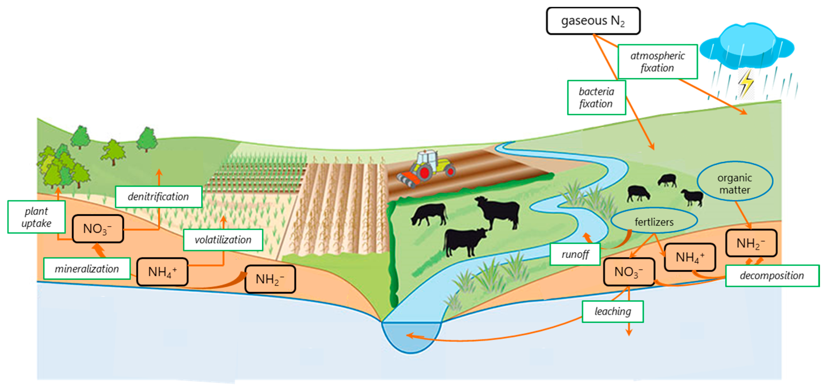
1. Introduction

Nitrogen-nitrate, while being fundamental for crop production, is of particular concern in the agricultural sector, as it can easily leach to the water table, worsening groundwater quality. Nitrate pollution of water is a major issue worldwide (Mateo-Sagasta et al., 2018; Wang and Li 2019; Zhang et al., 2019) [1,2,3]. It originates mostly from the use of inorganic fertilizers and animal manure in agricultural areas (Liao et al., 2012; Nakagawa et al., 2017; Ward et al., 2018; Zhang et al., 2018a) [4,5,6,7], and inefficient management of treated/untreated wastewater (Minnig et al., 2018) [8] and solid waste disposal (Wakida and Lerner 2005) [9]. Focusing on groundwater, nitrate contamination is a worldwide problem (Re et al., 2017; Zhang et al., 2018b; Ducci et al., 2019; Shukla and Saxena 2019) [10,11,12,13]. In Europe, policies to reduce NH₄⁺ and NO₃⁻ losses have been in place since nearly 30 years following the issue of the Nitrates Directive (ND; EC 1991) [14]. The ND objectives have been to reduce water pollution caused or induced by nitrates, and to prevent further pollution. According to the ND, Member States are asked to identify Nitrate Vulnerable Zones (NVZs), i.e., zones with eutrophic water bodies or at risk of eutrophication, with nitrate concentration in ground- or surface-water exceeding 50 mg/L (NO₃⁻ regulatory limit for drinking water; Wild et al., 2018 [15]). Anyway, Wild et al., (2018) [15] argue that it will take several decades to significantly reduce nitrate concentrations in porous aquifers via denitrification, even if future nitrate inputs were considerably reduced.

The ND was followed in 2000 by the Water Framework Directive (WFD; EC, 2000 [16]), whose goal is to reach a good chemical and ecological status of water bodies by 2027. The purposes, objectives, and strategies of the WFD overlap with those of the ND, especially after the introduction of the Groundwater Directive (EC, 2006 [17]) in 2006. In the attempt to target the objectives of the above-mentioned directives, River Basin Management Plans envisage approaches to assess nitrogen occurrence and to evaluate the effectiveness of measures to reduce nitrogen content in groundwater. Such approaches include monitoring of groundwater quality in NVZs (e.g., Jørgensen et al., 2009 [18]) and evaluation of nitrate leaching through the unsaturated zone and nitrate fate and transport in surface- and ground-water by means of modeling (e.g., Pistocchi et al., 2012; Klement et al., 2018; Husic et al., 2019 [19,20,21]).

The nitrogen cycle (Figure 1) involves physical, chemical, and biological processes which determine an increase or decrease of nitrogen content in the soil and the vadose zone, as well as nitrogen transformation among organic nitrogen (NH₂⁻), ammonium (NH₄⁺) and nitrate (NO₃⁻) pools. Three sub-cycles may be distinguished:

• the sub-cycle occurring in the atmosphere;
• the sub-cycle occurring in the unsaturated zone;
• the sub-cycle occurring in the plants, which involves NO₃⁻ uptake by roots.

Sources/sinks contributing to the three nitrogen pools also play relevant roles (e.g., deriving from surface runoff, fertilizers, etc.). A detailed review on the N cycle in the vadose zone-groundwater system may be found in Xin et al., (2019) [22].

Several models are available to simulate watershed/field scale hydrological processes. Some of these models also include methods to simulate the nitrogen cycle in soils and nitrogen leaching, the downward transport of N passing the root zone by percolating water through the unsaturated zone (Golmohammadi et al., 2014 [23]). Appendix A reports the main characteristics of some of these models, in terms of the modeling approach adopted (lumped or spatially distributed), the scale of application, and space and time discretization. Details about the mathematical approach are reported as well, focusing on the hydrological and the nitrogen cycling components only.

Most of the codes listed in Appendix A include a hydrological component, except for ANIMO (Groenendijk and Kroes 1999 [24]), which can be coupled to external models (e.g., SIMGRO, Querner and Van Bakel 1989 [25]; SWAP, Van Dam et al., 1997 [26]) for the simulation of water fluxes and moisture contents. In ANIMO, such components are then algebraically summed to get the change in water volume over time, to be used as input in the nitrogen cycling component. In EPIC (Sharpley 1990 [27]), APEX (Williams et al., 2015 [28]) and SWAT (Neitsch et al., 2005 [29]), belonging to the CREAMS (Knisel 1980 [30]) family of models, the hydrological component is based on algebraic mass balance equations involving rainfall, runoff, and evapotranspiration and other hydrological processes. On the other hand, other codes (i.e., DAISY, Hansen et al., 1990 [31]); PRZM-3, Suárez 2005 [32]; and NTT-Watershed, Heng and Nikolaidis 1998 [33]) solve the Richards’ equation for soil water dynamics in the unsaturated zone.

Regarding the nitrogen cycling component, all the codes reported in Appendix A integrate equations for the simulation of the processes involved in the nitrogen cycle. DAISY and PRZM-3 simulate NH₂⁻ mineralization in a very detailed way, including different NH₂⁻ sub-pools and resulting in large-parameterized models. EPIC, APEX, and SWAT use soil-dependent decay coefficients for the simulation of nitrogen leaching through the unsaturated zone, while ANIMO, DAISY, PRZM-3, and NTT-Watershed solve 1D advection-dispersion solute transport equations in the unsaturated zone.

Nitrate leaching research grew in the scientific community in the last decades (Padilla et al., 2018 [34]), focusing also on modeling methodologies (Canter 2019 [35]). Indeed, assessing nitrogen transport and turnover in the unsaturated zone and in groundwater is an expensive and complex task to be run at field scale (Sutton et al., 2011 [36]). At the same time, advances in distributed modeling efforts that incorporate spatial distribution of nitrogen inputs, soil and aquifer characteristics, land use data, and farming practices are promising (Xu et al., 2013; Ransom et al., 2017 [37,38]). While several modeling studies focused on simulating soil nitrogen balance or groundwater nitrogen transport independently (Wriedt 2004 [39]; Epelde et al., 2016 [40]), there is a clear trend to combine unsaturated zone and groundwater flow models for the simulation of nitrogen dynamics [41,42,43].

As such, in the following sections, we present a new modeling approach in order to compute nitrate leaching to the water table based on (a) the development of a numerical module for the simulation of the nitrogen cycle in the unsaturated zone, (b) the integration of such module in the Geographic Information System (GIS)-integrated FREEWAT platform (Foglia et al., 2018 [44]). The module was developed taking steps from the ANIMO and EPIC lumped models. Once developed, the module was then coupled to physically-based, spatially distributed codes for the simulation of unsaturated zone flow and agricultural water management and, finally, included into the GIS-integrated FREEWAT platform.

2. Materials and Methods

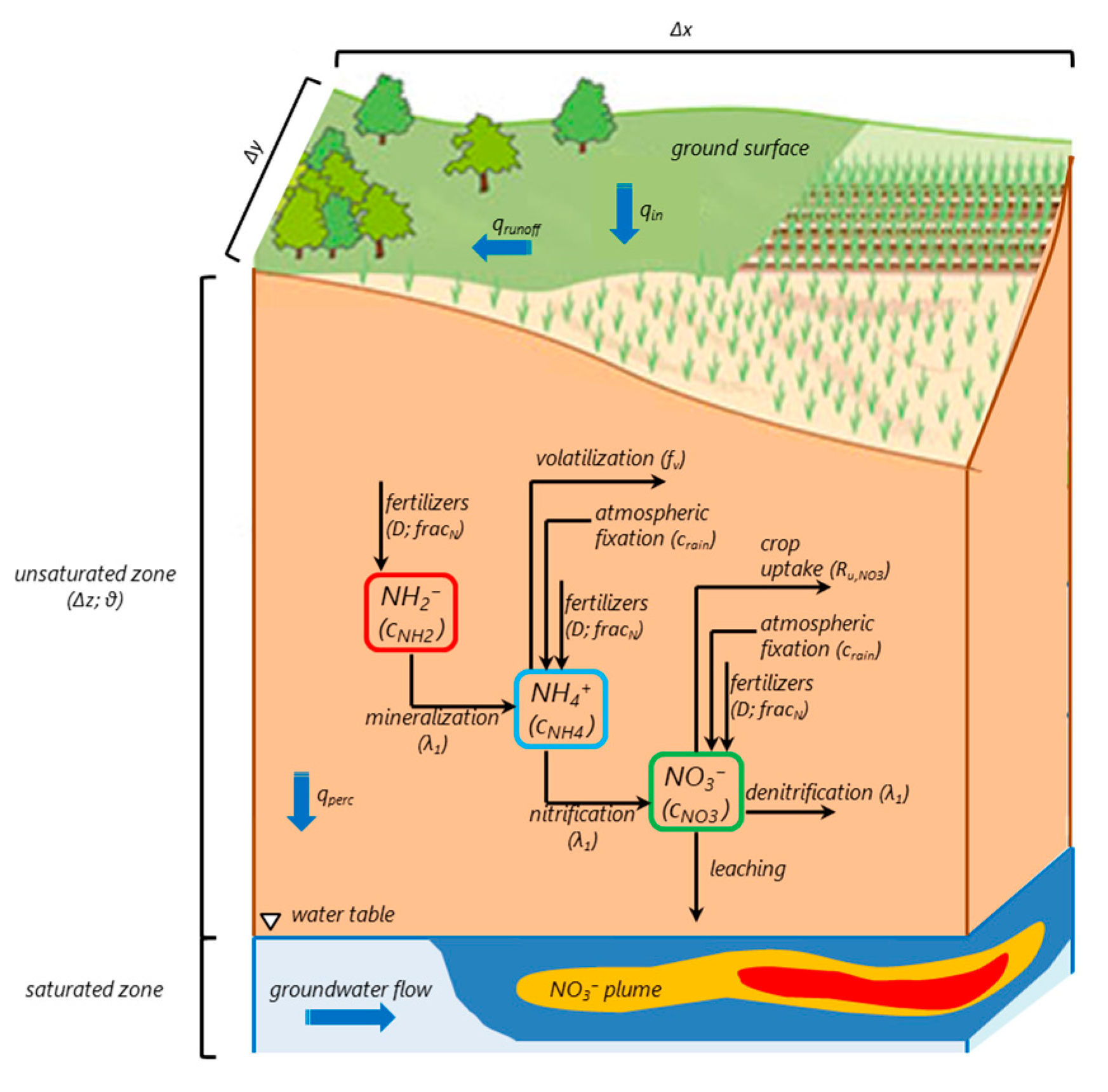
2.1. Overview of the Nitrogen Cycle Module

The nitrogen cycle module here developed allows to simulate the processes determining an increase or decrease of nitrogen content in the unsaturated zone, as well as nitrogen transformation among the NH₂⁻, NH₄⁺, and NO₃⁻ pools (Figure 1). The module developed is based on the conceptualization of the ANIMO model [24]. ANIMO simulates the nitrogen budget for the three pools, by solving a partial differential equation for each of them (

Table 1. Partial differential equations solved by the ANIMO model for the three nitrogen pools (modified after Groenendijk and Kroes 1999 [24]).

Nitrogen Pool	Conservation Term		Vertical Flow Term	Lateral Outflow Term	Crop Uptake Term	Decomposition Term	Production Term
NH2−	$\frac{\partial \left(\theta \left(t\right)c_{NH2}\left(t\right)\right)}{\partial t}$	=	$-\frac{\partial J_{s,NH2}\left(t,z\right)}{\partial z}$	$-R_{x,NH2}\left(t\right)$		$-R_{d,NH2}\left(t\right)$	$+R_{p,NH2}\left(t\right)$
NH4+	$\frac{\partial \left(\theta \left(t\right)c_{NH4}\left(t\right)\right)}{\partial t}+{\rho }_d\frac{\partial X_{e,NH4}\left(t\right)}{\partial t}$	=	$-\frac{\partial J_{s,NH4}\left(t,z\right)}{\partial z}$	$-R_{x,NH4}\left(t\right)$	$-R_{u,NH4}\left(t\right)$	$-R_{d,NH4}\left(t\right)$	$+R_{p,NH4}\left(t\right)$
NO3−	$\frac{\partial \left(\theta \left(t\right)c_{NO3}\left(t\right)\right)}{\partial t}$	=	$-\frac{\partial J_{s,NO3}\left(t,z\right)}{\partial z}$	$-R_{x,NO3}\left(t\right)$	$-R_{u,NO3}\left(t\right)$	$-R_{d,NO3}\left(t\right)$	$+R_{p,NO3}\left(t\right)$

). All terms and symbols listed in Table 1 are detailed in Appendix B and Appendix C. Figure 2 reports a sketch of all the processes related to nitrogen mass flux in the unsaturated zone, occurring within a grid cell. By solving the equations reported in Table 1, the variation of nitrogen concentration for each pool in time and space, in the unsaturated zone, is calculated.

The following terms appear in the equations presented in Table 1:

• a conservation term, which expresses the variation of nitrogen concentration in time;
• the conservation term for NH4+ includes also sorption by soil $({\rho }_d\frac{\partial X_{e,NH4}\left(t\right)}{\partial t})$;
• a vertical, unidimensional transport term, which is driven by unsaturated zone flow;
• a term related to lateral movement of nitrogen in the unsaturated zone (lateral outflow term). However, in our approach, we assume that vertical transport of nitrogen is the predominant process. As such, lateral movement of nitrogen is not simulated;
• a crop uptake term for NO₃⁻ and NH₄⁺. Such term is estimated for NO₃⁻ only, adopting the EPIC model approach (Sharpley 1990) [27], taking into account the phenological phases of crops. We assume, indeed, that NO₃⁻ is the predominant form of available nitrogen uptaken by roots (Nadelhoffer et al., 1984; Xu et al., 2012) [45,46];
• a decomposition term, i.e., mineralization for NH₂⁻, nitrification for NH₄⁺, denitrification for NO₃⁻;
• a production/loss term, which includes source/sink terms for each pool and the decomposition term from the above pool (i.e., NH₂⁻ represents the pool above NH₄⁺, and NH₄⁺ represents the pool above NO₃⁻).

The relation among the three pools is guaranteed through the decomposition mechanisms:

(a)

mineralization of organic nitrogen represents a sink term for the NH₂⁻ pool and a source term for the NH₄⁺ pool. As such, this is subtracted in the decomposition term for NH₂⁻ (R_(d,NH2) in Table 1) and summed as production term for NH₄⁺ (R_(p,NH₄) in Table 1);

(b)

nitrification of ammonium represents a sink term for the NH₄⁺ pool and a source term for the NO₃⁻ pool. As such, this is subtracted in the decomposition term for NH₄⁺ (R_(d,NH₄) in Table 1) and summed as production term for NO₃⁻ (R_(p,NO₃) in Table 1).

The equations reported in Table 1 are solved one by one, in the order presented above. Each of them can be rewritten as (subscripts NH₂, NH₄ and NO₃ will be omitted in the following):

$$\left[\theta \left(t_0\right)+\phi \Delta t+{\rho }_d{K}_d\right]\frac{dc\left(t\right)}{dt}=\frac{q_{in}\left(t\right)\left[c_{rain}\left(t\right)+c\left(t_0\right)\right]}{\Delta z}-\frac{q_{perc}\left(t\right)c\left(t\right)}{\Delta z*\Delta x*\Delta y}-K_{up}c\left(t\right)-{\lambda }_1\theta \left(t\right)c\left(t\right)+R_p-\phi c\left(t\right)$$

(1)

By solving Equation (1), concentration in time (c(t)) for each pool is calculated in the unsaturated zone at the time t.

We decided to take steps from the ANIMO, among the models listed in the Appendix A, because we considered it a good compromise with respect to the following aspects:

-

the mathematical approach adopted, based on the mass conservation and the solution of transport Equation (1);

-

the mathematical approach adopted is relatively frugal, in the sense that it requires few input parameters;

-

the integration between Equation (1) and the unsaturated zone flow term calculated by means of distributed models integrated within the FREEWAT platform was pretty straightforward with respect to the space and time dimension of the involved processes.

2.2. Overview of the FREEWAT Platform

FREEWAT [47] is a free and open source platform integrated in a GIS framework for water resource management, with a specific focus on groundwater, initially developed within the HORIZON 2020 FREEWAT project (FREE and open source software tools for WATer resource management; www.freewat.eu; [48]), a follow up of the SID&GRID platform [49].

FREEWAT is conceived as a QGIS [50] plugin, which integrates free and open source software tools for pre- and post-processing of spatial data, and numerical codes for the simulation of the hydrological cycle. On one side, GIS and spatial database management applications [51] are exploited for spatial data storage, visualization and analysis. Physically-based and spatially distributed numerical models (i.e., MODFLOW, Harbaugh 2005 [52], and MODFLOW-related models) integrated within the FREEWAT platform allow to simulate several processes involved in the hydrological cycle (e.g., groundwater flow, density-dependent flow, conjunctive use of ground- and surface-water, solute transport, sensitivity analysis and model calibration). Dedicated tools for pre-processing of field data [53,54] and for post-processing of models’ results are integrated as well. FREEWAT was applied to date to a variety of case studies [55]. The present work may be considered as a continuation of the research activities performed to better describe agricultural water use in hydrological modelling. In particular, the Farm Process (FMP; embedded in the USGS’s MODFLOW One-Water Hydrologic Model [56]) coupled to a Crop Growth Model (CGM [57]) for simulating crop yield based on solar radiation and biomass accumulation was previously integrated within the FREEWAT platform.

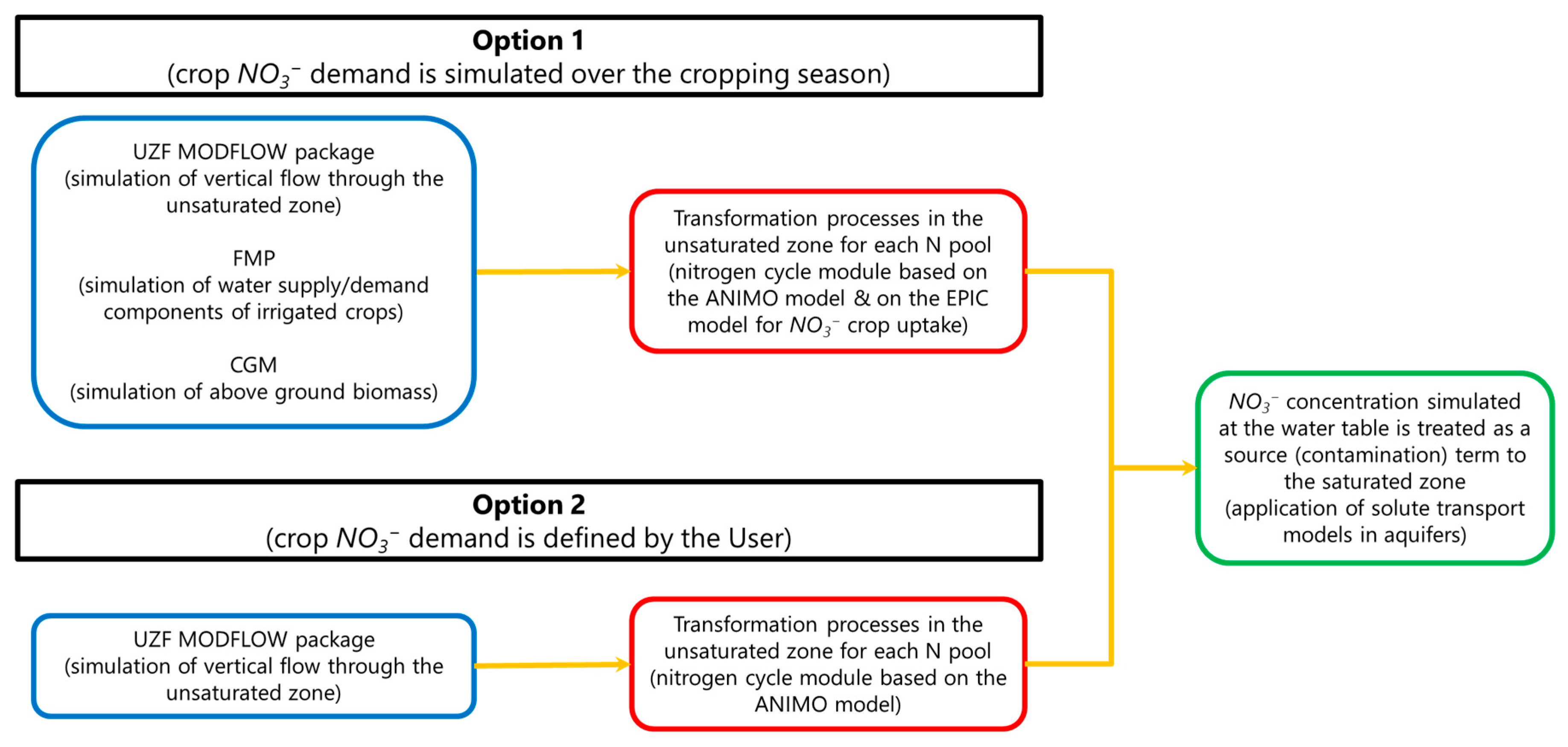
2.3. Coupling the Nitrogen Cycle and the Hydrological One

The nitrogen cycle module was coupled to the unsaturated flow process, in order to simulate advective transport of nitrogen compounds in the downward direction, across the unsaturated zone. According to the ANIMO approach, the nitrogen concentration in the outflowing water, moving from one unsaturated zone layer to another, is equal to the calculated nitrogen concentration within the ith unsaturated zone layer [24]. In our approach, by activating the Unsaturated Zone Flow (UZF) MODFLOW package [58] in a groundwater flow model based on MODFLOW-2005 [52], we simulate a fraction of the total nitrogen mass within the unsaturated zone that reaches the water table. The nitrogen mass flow is driven by vertical water flow through the unsaturated zone. The UZF solves a kinematic wave approximation of the Richards’ equation to simulate vertical flow and storage through the unsaturated zone [58]. Conversely from most of the lumped available codes simulating the nitrogen cycle (e.g., ANIMO and EPIC), the codes integrated in the FREEWAT platform for the simulation of the unsaturated zone are spatially distributed. Hence, the partial differential equations are solved to get the involved variables (e.g., hydraulic head and solute concentration) also in a discretized space.

The coupling approach includes agricultural water management processes for the representation of inorganic nitrogen uptake by plants’ roots. To this scope, the coupled FMP-CGM approach developed in FREEWAT for agricultural water management and crop yield simulation is adopted: in the nitrogen cycle module, input and output of an FMP-CGM scenario are used to calculate NO₃⁻ crop demand, as conceptualized in the EPIC model [27]. Specifically, NO₃⁻ crop demand over the different phases of the cropping season is calculated in EPIC as the difference between the NO₃⁻ crop content, which is the nitrogen amount in plant biomass, and the NO₃⁻ availability in the soil. Crop transpiration fluxes simulated by FMP and cumulated biomass calculated by CGM are involved in the computation of these two variables.

All of the processes involved in the nitrogen cycle were simulated in the unsaturated zone layer at each cell of a finite-difference grid. This allows to obtain the spatial variation of nitrogen concentration for each nitrogen pool in the unsaturated zone.

The coupling approach just presented is drawn in Figure 3. The left side of Figure 3 (blue boxes) reports the codes that must be run before running the nitrogen cycle module. Two options may occur:

-

if crop NO₃⁻ demand is simulated over the cropping season (Option 1), the following is needed:

• running a MODFLOW-2005 model, including the UZF Package, to simulate water flow through the unsaturated zone. This is needed for the calculation of the thickness of the unsaturated zone, the water content, the runoff rate and the leaching rate in space and time;
• running an FMP-CGM scenario. This is needed for the calculation of crop transpiration flux and cumulated above-ground biomass;

-

if crop NO₃⁻ demand is not simulated, but the User inputs crop NO₃⁻ requirement parameters over the cropping season (Option 2). In such case, only running a MODFLOW-2005 model, including the UZF Package, is needed to simulate water flow through the unsaturated zone as above-mentioned.

The center of Figure 3 (red boxes) reports the simulated nitrogen cycle processes:

-

if Option 1 occurs, all of the processes involved in the nitrogen cycle are simulated taking steps from the ANIMO model approach, except for the NO₃⁻ crop uptake process, which is simulated through a sub-routine based on the EPIC model approach;

-

if Option 2 occurs, all the processes involved in the nitrogen cycle are simulated taking steps from the ANIMO model approach. In such case, the sub-routine based on the EPIC model approach is not executed, and the NO₃⁻ crop uptake process is simulated by comparing the crop NO₃⁻ requirement defined by the User with the NO₃⁻ availability in the unsaturated zone.

In both options, input/output parameters involved in the execution of the UZF, FMP, and CGM components are exploited to run the nitrogen cycle module (i.e., to solve Equation (1)). As a result, the NO₃⁻ concentration at the water table is determined at each cell and for each stress period. This concentration can then be treated as a potential contaminant source term to the saturated zone in solute transport modelling of aquifers (e.g., through the application of the MT3DMS code [59]), as indicated in the green box on the right side of Figure 3.

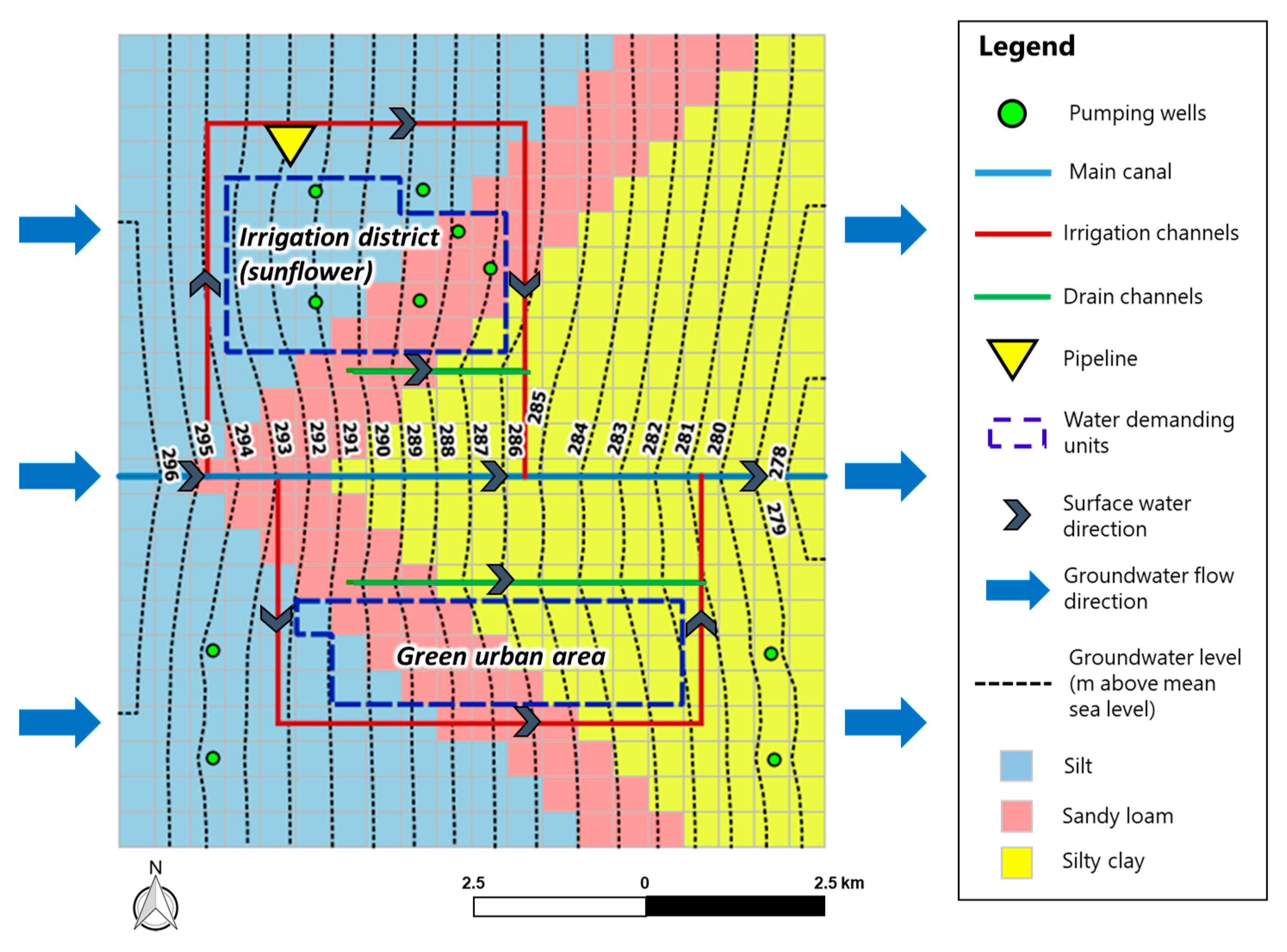
2.4. Model Testing Using a Synthetic Case Study

The coupling approach discussed in this paper was tested using a synthetic case study presented in Rossetto et al., (2019) [57]. There, the FMP-CGM methodology was applied for simulating daily conjunctive use of ground- and surface-water for the irrigation of sunflower. Sunflower yield at harvest was estimated based on crop phenology, climate conditions, and water availability. Here, we coupled the nitrogen module to that case study in order to exploit settings and results of the above-mentioned model. We focused our attention on the sunflower irrigated Water Demand Unit. Model settings are described in the following and reported in Figure 4.

The whole model extends over an area of 115 km² and it is discretized by means of square cells with 500 m of side length. For the calculation of sunflower water root uptake, root depth values and capillary fringe for the three soil types (silt, silty clay, and sandy loam) are assigned. Groundwater is pumped from a sandy aquifer represented through a homogeneous, MODFLOW convertible model layer with variable thickness. Groundwater is delivered to the irrigation district by six pumping wells. Groundwater flow occurs from west to east. The model was run in transient conditions between 1 January and 31 October 2017, with daily stress periods. Irrigation of sunflower was simulated following sunflower seeding on 1 April and up to 31 August 2017 (when the crop was harvested). During the crop growth the cumulated rainfall depth was 99.8 mm, mainly distributed over four rainfall events occurring between April and August. Model results showed that sunflower water demand is primarily met by precipitation and root uptake, and secondly by irrigation water. Further information on the case study may be found in Rossetto et al., (2019) [57].

The nitrogen cycle module was applied to the present case study to simulate daily nitrate leaching to the water table.

In order to solve Equation (1) for the NH₂⁻, NH₄⁺ and NO₃⁻ pools, initial concentration for each nitrogen compound was defined according to the total content of nitrogen in the soil and to the soil type. The following equations were used for such estimation (Masoni 2010) [60]:

$$c_{N{H}_2^{-}}\left(t_0=0\right)=0.95 {\rho }_a{N}_T$$

(2)

$$c_{N{H}_4^{+}}\left(t_0=0\right)=0.04 {\rho }_a{N}_T$$

(3)

$$c_{N{O}_3^{-}}\left(t_0=0\right)=0.01 {\rho }_a{N}_T$$

(4)

For the application of Equations (2)–(4) we assumed: N_T = 10⁻³ kg/kg (Masoni 2010) [60], ρ_a = 1360 kg/m³ for silt, ρ_a = 1440 kg/m³ for sandy loam, and ρ_a = 1200 kg/m³ for silty clay (Yu et al., 1993) [61].

This resulted in an initial concentration in the irrigation district ranging between 1140 mg/L and 1368 mg/L for NH₂⁻, between 48 mg/L and 58 mg/L for NH₄⁺, and between 12 mg/L and 14 mg/L for NO₃⁻.

Nitrogen concentration in rain water varies according to the intensity of precipitation. Figure 5 reports the content of NH₄⁺ and NO₃⁻ in rain water over the simulation (Eriksson 1952) [62], compared to the cumulated rainfall. Peak values of the nitrogen content in rain water were input when rainfall events occurred.

Decomposition processes for each nitrogen pool were simulated assuming that the first order decay rate constant (λ₁) was equal to 0.01 day⁻¹ (Groot et al., 2012) [63]. As a consequence, here we assumed that mineralization, nitrification, and denitrification contribute to a 1% daily decrease of NH₂⁻, NH₄⁺ and NO₃⁻ content, respectively.

Moreover, NH₄⁺ volatilization and sorption were simulated. We assumed that the volatilization fraction (f_v) was equal to 0.001. For simulating sorption, we used the same values as the apparent density for ρ_d, and the following values for the Cation Exchange Capacity (CEC): 148 meq/kg for silt, 110 meq/kg for sandy loam, 146 meq/kg for silty clay [64].

For simulating nitrate uptake by sunflower roots over the cropping season, we exploited results from the FMP-CGM model presented in [57]. As such, we adopted the approach based on the EPIC conceptualization, by setting the following for sunflower [27]: bn₁ = 0.05, bn₂ = 0.023, bn₃ = 0.0146, PHU = 1600.

In order to define the N fertilizer rate to be applied for achieving the simulated sunflower yield, we applied a conventional N balance approach, as

N_f = N_d − (N_r + N_i + N_m) + (N_l + N_v + N_de) ± N_p

(5)

where N_f is N fertilizer rate, N_d is crop N demand, N_r is N supplied by rainfall, N_i is N supplied by irrigation, N_m is mineralized N from soil organic matter, N_l is N loss from leaching, N_v is N loss from volatilization, N_de is N loss from denitrification, and N_p is N released (positive) or taken from soil (negative) for residue decomposition of the preceding wheat crop. All terms in the equation are expressed as kg N ha⁻¹.

Sunflower N demand (N_d) for 5 Mg ha⁻¹ grain yield with 3.3% grain N concentration, harvest index 0.4 and 1.0% residue N concentration is 240 kg N ha⁻¹. Nitrogen supply from rainfall and irrigation was 2 and 23.5 kg ha⁻¹, respectively, and from soil organic matter mineralization was 36.8 kg ha⁻¹ from the silt soil and 43.6 kg ha⁻¹ from the sandy-loam soil. Nitrogen loss from leaching, denitrification, and volatilization were assumed to be negligible. Indeed, the amount of irrigation was calculated to avoid percolation and since soils are well drained, they do not offer favorable anaerobic conditions for denitrification. Finally, we assume negligible NH₃ emissions occur with soil incorporation of urea (Rochette et al., 2013) [65].

Consequently, N_f was estimated 185.6 kg N ha⁻¹ for the silt soil and 178.8 kg N ha⁻¹ for the sandy-loam soil. We then applied the following values for the dose of fertilization: D = 1.856 × 10⁻² kg/m² for silt and D = 1.788 × 10⁻² kg/m² for sandy loam. Such values were assigned the day before the beginning of the sunflower cropping season (31 March), and the whole amounts were assigned to the NH₂⁻ pool only ($fra{c}_{NH2}$ = 1; $fra{c}_{NH4}$ = 0; $fra{c}_{NO3}$ = 0).

Table 2. Values set for the input parameters in the case study.

Parameter	Units of Measurements	Value
NT	kg/kg	10−3
ρa and ρd	kg/m3	1360 (silt) 1440 (sandy loam) 1200 (silty clay)
λ1	day−1	10−2
fv		10−3
CEC	meq/kg	148 (silt) 110 (sandy loam) 146 (silty clay)
bn1		0.05
bn2		0.023
bn3		0.0146
PHU		1600
D	kg/m2	1.856 × 10−2 (silt) 1.788 × 10−2 (sandy loam)
$fra{c}_{NH2}$		1
$fra{c}_{NH4}$		0
$fra{c}_{NO3}$		0

presents the dataset used.

3. Results and Discussion

The simulation performed allowed us to estimate daily concentration values of NO₃⁻ arriving at the water table. Figure 6 presents the daily values of NO₃⁻ concentration simulated at the water table over the simulation period, with respect to the simulated effective rainfall infiltration through the unsaturated zone. We can notice that leaching occurs before the crop seeding (between early February and early April 2017) and then around mid-September 2017. These leaching events are mostly related to rainfall events concentrated in those periods (Figure 5 and Figure 6). On February–April 2017, daily NO₃⁻ concentration reaching the water table may reach values up to about 1 mg/L, while values up to about 1.3 mg/L were simulated on mid-September 2017. From the results of the simulation, we explain the relatively high concentration arriving at the water table following rainfall events before the crop season due to the absence of the crop uptake term—similarly, such concentration increases at the end of the crop season, after crop harvesting (that is, no more crop nitrogen uptake). On the other hand, during the sunflower cropping season (April to end of August), the daily NO₃⁻ concentration values at the water table have very low values (in the order of 10⁻³ mg/L), as a result of the drought period simulated and of crop uptake (Figure 6). Our results show a potential risk of NO₃⁻ leaching during the winter wet season. Moreover, substantial NO₃⁻ leaching losses may be due to high-intensity rainfalls, such as the one occurred in September 2017. Unfortunately, data coming from experimental activities about daily concentration of NO₃⁻ arriving at the water table are not published yet—and because of this it was not possible to validate the simulated values.

The time-varying simulated data in Figure 6 refers to one single point in space. Figure 7 shows the spatial distribution of NO₃⁻ concentrations arriving at the water table. At the selected time nitrogen crop demand is high. The available nitrogen is uptaken through the roots, and, as result of the simulation, we have very low values of NO₃⁻ concentrations arriving at the water table. These concentration values may then be used to define the time and spatially variant source term for simulation of nitrate transport in aquifers (e.g., using the MT3DMS code [59]).

The coupling approach presented holds the following limitations:

-

the unsaturated zone is discretized in only one layer. It is then considered as a unique layer extending from the ground surface to the water table. This representation may not be suitable in case of non-homogeneous soil sediments, with different physical and chemical properties. Furthermore, NO₃⁻ uptake at different depths according to the root distribution in the vertical domain may not be adequately reproduced;

-

purely advective transport of nitrogen through the unsaturated zone is simulated (dispersion is neglected);

-

the biological fixation process is not simulated. This can lead to underestimation of mineral nitrogen available in the soil;

-

volatilization of NH₄⁺ is taken into account through a volatilization coefficient (f_v) only, which is difficult to quantify;

-

NH₄⁺ uptake by plants’ roots is not simulated (we assume, indeed, that NO₃⁻ is the predominant form of available nitrogen uptaken by roots);

-

taking steps from the UZF MODFLOW package approach, we assume that vertical movement of nitrogen is the predominant process. As such, lateral movement of nitrogen across neighboring cells is not simulated;

-

when the thickness of the unsaturated zone varies, according to water level fluctuations, the mass of nitrogen stored in the soil is simply redistributed over the whole unsaturated thickness.

Due to the number of required parameters, reduced compared to other simulation methods, but still very large, we were only able to validate this approach by means of a synthetic case study. Validation by means of real data is however needed, i.e., to verify in a real environment the processes that lead to the low concentration values in Figure 7. Indeed, coupling the nitrogen to the hydrological cycle means, when coming to model validation, to get data on the hydrology, the crop growth and nitrate cycle at the same time, which is more than 50 parameter’s values required (see Appendix B for details) with related uncertainties evaluation. In this sense, experimental trials ranging from lysimeters to field scale pilot (as in [66,67,68]), even with high-resolution lysimeters [69] may allow to get the required data. Dedicated field scale experiments, where longer flowpaths through the unsaturated zone may be taken into account, using also state-of-the art ground and remote sensors will allow to complete the validation of the presented approach.

4. Conclusions

Agriculture-related activities very often cause leaching of high levels of nutrients in the soil and the connected aquatic ecosystems, including groundwater. Among nutrients, nitrate is of particular concern, as it is conservative and it may rapidly leach to the water table, causing high, or even exceeding, according to ongoing regulations, concentrations in aquifers and, consequently, potential negative effects on the environment and even human health, in case groundwater is used for drinking purposes.

In this paper, we described the development of a nitrogen module for the simulation of the nitrogen cycle in the unsaturated zone and the nitrate leaching process. The developed module takes steps from the mathematical framework of the ANIMO model, which solves a mass conservation and transport equation for dissolved organic nitrogen, nitrate, and ammonium to quantify the relation between fertilization, soil management and nutrients leaching occurring over time in a vertical soil column. The simulation of nitrate crop demand and root uptake, instead, is based on the more robust conceptualization of the EPIC model, which accounts for the different phases of the cropping season to calculate crop nitrate content and need.

We integrated the developed nitrogen cycle module within the GIS-based FREEWAT platform, in order to couple it with the spatially distributed codes (e.g., MODFLOW) for the simulation of unsaturated zone and groundwater flow processes. Thanks to the integration, we exploited inputs and outputs from the hydrological models to test the developed modules for simulating the processes involved in the nitrogen cycle. To do so, the nitrogen cycle module was developed to run at each cell and for the same stress periods of a MODFLOW model previously set. More specifically, the developed module exploits results from the UZF MODFLOW package for getting the water content and thickness of the unsaturated zone, and infiltration and runoff rates generated during rainfall events. Moreover, results from an agricultural water management scenario based on the application of FMP-CGM are used to determine the nitrate demand by crops over the growing season.

The coupling approach just summarized guarantees the possibility to implement nitrogen cycle scenarios requiring relatively few inputs. The simulate daily nitrate concentration at the water table distributed in space is the main relevant output derived from this simulation approach.

The presented effort is an initial stage of research in producing usable numerical tools for improving nitrogen management in agricultural fields. Further development of the code may include, among the others, the integration of lateral movement of nitrogen between neighboring cells, and the simulation of root uptake with a finer vertical discretization based on root depth and distribution.

References

- Mateo-Sagasta, J.; Zadeh, S.M.; Turral, H. More People, More Food, Worse Water? A Global Review of Water Pollution from Agriculture; FAO: Rome, Italy; International Water Management Institute (IWMI), CGIAR Research Program on Water, Land and Ecosystems (WLE): Colombo, Sri Lanka, 2018. [Google Scholar]
- Wang, Z.; Li, S.-X. Nitrate N loss by leaching and surface runoff in agricultural land: A global issue (a review). Adv. Agron. 2019, 156, 159–217. [Google Scholar] [CrossRef]
- Zhang, Y.; Shi, P.; Song, J.; Li, Q. Application of Nitrogen and Oxygen Isotopes for Source and Fate Identification of Nitrate Pollution in Surface Water: A Review. Appl. Sci. 2018, 9, 18. [Google Scholar] [CrossRef]
- Liao, L.; Green, C.T.; Bekins, B.A.; Böhlke, J.K. Factors controlling nitrate fluxes in groundwater in agricultural areas. Water Resour. Res. 2012, 48. [Google Scholar] [CrossRef]
- Nakagawa, K.; Amano, H.; Takao, Y.; Hosono, T.; Berndtsson, R. On the use of coprostanol to identify source of nitrate pollution in groundwater. J. Hydrol. 2017, 550, 663–668. [Google Scholar] [CrossRef]
- Ward, M.H.; Jones, R.R.; Brender, J.D.; De Kok, T.M.; Weyer, P.J.; Nolan, B.T.; Villanueva, C.M.; Van Breda, S.G. Drinking Water Nitrate and Human Health: An Updated Review. Int. J. Environ. Res. Public Health 2018, 15, 1557. [Google Scholar] [CrossRef]
- Zhang, Y.; Shi, P.; Li, F.; Wei, A.; Song, J.; Ma, J. Quantification of nitrate sources and fates in rivers in an irrigated agricultural area using environmental isotopes and a Bayesian isotope mixing model. Chemosphere 2018, 208, 493–501. [Google Scholar] [CrossRef]
- Minnig, M.; Moeck, C.; Radny, D.; SchirmeriD, M. Impact of urbanization on groundwater recharge rates in Dübendorf, Switzerland. J. Hydrol. 2018, 563, 1135–1146. [Google Scholar] [CrossRef]
- Wakida, F.T.; Lerner, D.N. Non-agricultural sources of groundwater nitrate: A review and case study. Water Res. 2005, 39, 3–16. [Google Scholar] [CrossRef]
- Re, V.; Sacchi, E.; Kammoun, S.; Tringali, C.; Trabelsi, R.; Zouari, K.; Daniele, S. Integrated socio-hydrogeological approach to tackle nitrate contamination in groundwater resources. The case of Grombalia Basin (Tunisia). Sci. Total Environ. 2017, 593, 664–676. [Google Scholar] [CrossRef]
- Zhang, Q.; Wang, H.; Wang, L. Tracing nitrate pollution sources and transformations in the over-exploited groundwa-ter region of north China using stable isotopes. J. Contam. Hydrol. 2018, 218, 1–9. [Google Scholar] [CrossRef]
- Ducci, D.; Della Morte, R.; Mottola, A.; Onorati, G.; Pugliano, G. Nitrate trends in groundwater of the Campania region (southern Italy). Environ. Sci. Pollut. Res. 2019, 26, 2120–2131. [Google Scholar] [CrossRef] [PubMed]
- Shukla, S.; Saxena, A. Global Status of Nitrate Contamination in Groundwater: Its Occurrence, Health Impacts, and Mitigation Measures. In Handbook of Environmental Materials Management; Springer: Cham, Switzerland, 2019; pp. 869–888. [Google Scholar] [CrossRef]
- European Commission. Concerning the Protection of Waters Against Pollution Caused by Nitrates from Agricultural Sources; Directive of the Council of 12 December 1991; European Commission: Brussels, Belgium, 1991. [Google Scholar]
- Wild, L.M.; Mayer, B.; Einsiedl, F. Decadal Delays in Groundwater Recovery from Nitrate Contamination Caused by Low O2Reduction Rates. Water Resour. Res. 2018, 54, 9996. [Google Scholar] [CrossRef]
- European Commission. Establishing a Framework for the Community Action in the Field of Water Policy; Directive 2000/60/EC of the European Parliament and of the Council of 23 October 2000; European Commission: Brussels, Belgium, 2000. [Google Scholar]
- European Commission. Protection of Ground Water against Pollution and Deterioration; Directive 2006/118/EC of the European Parliament and the Council of 12 December 2006; European Commission: Brussels, Belgium, 2006. [Google Scholar]
- Jørgensen, L.F.; Stockmarr, J. Groundwater monitoring in Denmark: Characteristics, perspectives and comparison with other countries. Hydrogeol. J. 2008, 17, 827–842. [Google Scholar] [CrossRef]
- Pistocchi, C.; Silvestri, N.; Rossetto, R.; Sabbatini, T.; Guidi, M.; Baneschi, I.; Bonari, E.; Trevisan, D. A Simple Model to Assess Nitrogen and Phosphorus Contamination in Ungauged Surface Drainage Networks: Application to the Massaciuccoli Lake Catchment, Italy. J. Environ. Qual. 2012, 41, 544–553. [Google Scholar] [CrossRef] [PubMed]
- Klement, L.; Bach, M.; Breuer, L.; Nendel, C.; Kersebaum, K.C.; Stella, T.; Berg-Mohnicke, M. Modelling nitrate losses from agricultural land in Germany. EGU Gen. Assem. Conf. Abstr. 2018, 20, 14833. [Google Scholar]
- Husic, A.; Fox, J.; Adams, E.; Ford, W.; Agouridis, C.; Currens, J.; Backus, J. Nitrate pathways, processes, and tim-ing in an agricultural karst system: Development and application of a numerical model. Water Resour. Res. 2019, 55, 2079–2103. [Google Scholar] [CrossRef]
- Xin, J.; Liu, Y.; Chen, F.; Duan, Y.; Wei, G.; Zheng, X.; Li, M. The missing nitrogen pieces: A critical review on the distribution, transformation, and budget of nitrogen in the vadose zone-groundwater system. Water Res. 2019, 165, 114977. [Google Scholar] [CrossRef]
- Golmohammadi, G.; Prasher, S.O.; Madani, A.; Rudra, R.P. Evaluating Three Hydrological Distributed Watershed Models: MIKE-SHE, APEX, SWAT. Hydrology 2014, 1, 20–39. [Google Scholar] [CrossRef]
- Groenendijk, P.; Kroes, J.G. Modelling the Nitrogen and Phosphorus Leaching to Groundwater and Surface Water with ANIMO 3.5 (No. 144); Winand Staring Centre: Wageningen, The Netherlands, 1999. [Google Scholar]
- Querner, E.P.; van Bakel, P.J.T. Description of the Regional Groundwater Flow Model SIMGRO; Report 7; DLO Winand Staring Centre: Wageningen, The Netherlands, 1989. [Google Scholar]
- Van Dam, J.C.; Huygen, J.; Wesseling, J.G.; Feddes, R.A.; Kabat, P.; van Walsum, P.E.V.; Groenendijk, P.; van Diepen, C.A. Simulation of Water Flow, Solute Transport and Plant Growth in the Soil-Water-Atmosphere-Plant Environment; Technical Document 45; DLO Winand Staring Centre: Wageningen, The Netherlands, 1997. [Google Scholar]
- Sharpley, A.N.; Williams, J.R. EPIC-erosion/productivity impact calculator: 1, Model Documentation. Tech. Bull. 1990, 1759, 235. [Google Scholar]
- Williams, J.R.; Izaurralde, R.C.; Williams, C.; Steglich, E.M. Agricultural Policy/Environmental eXtender Model. Theor. Doc. Vers. 2015, 604, 2008–2017. [Google Scholar]
- Neitsch, S.L.; Arnold, J.G.; Kiniry, J.R.; Williams, J.R.; King, K.W. Soil and Water Assessment Tool (SWAT): Theoretical Documentation, Version 2000; TWRI Report TR-191; Texas Water Resources Institute: College Station, TX, USA, 2002. [Google Scholar]
- Knisel, W.G. CREAMS: A Field Scale Model for Chemicals, Runoff, and Erosion from Agricultural Management Systems; Conservation Research Report 26; U.S. Department of Agriculture: Tucson, AZ, USA, 1980.
- Hansen, S.; Jensen, H.E.; Nielsen, N.E.; Svendsen, H. DAISY: A Soil Plant System Model. In Danish Simulation Model for Transformation and Transport of Energy and Matter in the Soil Plant Atmosphere System; The National Agency for Environmental Protection: Copenhagen, Denmark, 1990; p. 369. [Google Scholar]
- Suárez, L.A. PRZM-3, A Model for Predicting Pesticide and Nitrogen Fate in the Crop Root and Unsaturated Soil Zones: Users Manual for Release 3.12; U.S. Environmental Protection Agency (EPA): Washington, DC, USA, 2005.
- Heng, H.H.; Nikolaidis, N.P. MODELING OF NONPOINT SOURCE POLLUTION OF NITROGEN AT THE WATERSHED SCALE. J. Am. Water Resour. Assoc. 1998, 34, 359–374. [Google Scholar] [CrossRef]
- Padilla, F.M.; Gallardo, M.; Manzano-Agugliaro, F. Global trends in nitrate leaching research in the 1960–2017 period. Sci. Total Environ. 2018, 643, 400–413. [Google Scholar] [CrossRef] [PubMed]
- Canter, L.W. Nitrates in Groundwater; Informa UK Limited: London, UK, 2019; ISBN 9780367448455. [Google Scholar]
- Sutton, M.A.; Howard, C.M.; Erisman, J.W.; Billen, G.; Bleeker, A.; Grennfelt, P.; van Grinsven, H.; Grizzetti, B. The European Nitrogen Assessment: Sources, Effects and Policy Perspectives; Cambridge University Press: Cambridge, UK, 2011. [Google Scholar] [CrossRef]
- Xu, L.; Niu, H.; Xu, J.; Wang, X. Nitrate-Nitrogen Leaching and Modeling in Intensive Agriculture Farmland in China. Sci. World J. 2013, 2013, 1–10. [Google Scholar] [CrossRef] [PubMed]
- Ransom, K.M.; Bell, A.M.; Barber, Q.E.; Kourakos, G.; Harter, T. A Bayesian approach to infer nitrogen loading rates from crop and land-use types surrounding private wells in the Central Valley, California. Hydrol. Earth Syst. Sci. 2018, 22, 2739–2758. [Google Scholar] [CrossRef]
- Wriedt, G. Modelling of Nitrogen Transport and Turnover during Soil and Groundwater Passage in a Small Lowland Catchment of Northern Germany. Ph.D. Thesis, Universität Potsdam, Potsdam, Germany, 2004. [Google Scholar]
- Epelde, A.M.; Antiguedad, I.; Brito, D.; Jauch, E.; Neves, R.; Garneau, C.; Sauvage, S.; Sánchez-Pérez, J.M. Different modelling approaches to evaluate nitrogen transport and turnover at the watershed scale. J. Hydrol. 2016, 539, 478–494. [Google Scholar] [CrossRef]
- Almasri, M.N.; Kaluarachchi, J.J. Modeling nitrate contamination of groundwater in agricultural watersheds. J. Hydrol. 2007, 343, 211–229. [Google Scholar] [CrossRef]
- Jin, L.; Whitehead, P.G.; Heppell, C.M.; Lansdown, K.; Purdie, D.A.; Trimmer, M. Modelling flow and inorganic nitrogen dynamics on the Hampshire Avon: Linking upstream processes to downstream water quality. Sci. Total Environ. 2016, 572, 1496–1506. [Google Scholar] [CrossRef]
- Ikenberry, C.D.; Soupir, M.L.; Helmers, M.J.; Crumpton, W.G.; Arnold, J.G.; Gassman, P.W. Simulation of Daily Flow Pathways, Tile-Drain Nitrate Concentrations, and Soil-Nitrogen Dynamics Using SWAT. J. Am. Water Resour. Assoc. 2017, 53, 1251–1266. [Google Scholar] [CrossRef]
- Foglia, L.; Borsi, I.; Mehl, S.; de Filippis, G.; Cannata, M.; Vasquez-Sune, E.; Criollo, R.; Rossetto, R. FREEWAT, a Free and Open Source, GIS-Integrated, Hydrological Modeling Platform. Groundwater 2018, 56, 521–523. [Google Scholar] [CrossRef]
- Nadelhoffer, K.J.; Aber, J.D.; Melillo, J.M. Seasonal patterns of ammonium and nitrate uptake in nine temperate forest ecosystems. Plant Soil 1984, 80, 321–335. [Google Scholar] [CrossRef]
- Xu, G.; Fan, X.; Miller, A.J. Plant Nitrogen Assimilation and Use Efficiency. Annu. Rev. Plant Biol. 2012, 63, 153–182. [Google Scholar] [CrossRef] [PubMed]
- De Filippis, G.; Borsi, I.; Foglia, L.; Cannata, M.; Mansilla, V.V.; Suñé, E.V.; Ghetta, M.M.; Rossetto, R. Software tools for sustainable water resources management: The GIS-integrated FREEWAT platform. Rend. Online Soc. Geol. Ital. 2017, 42, 59–61. [Google Scholar] [CrossRef]
- Rossetto, R.; Borsi, I.; Foglia, L. FREEWAT: FREE and open source software tools for WATer resource management. Rend. Online Soc. Geol. Ital. 2015, 35, 252–255. [Google Scholar] [CrossRef]
- Rossetto, R.; Borsi, I.; Schifani, C.; Bonari, E.; Mogorovich, P.; Primicerio, M. SID&GRID: Integrating hydrological modeling in GIS environment. Rend. Online Soc. Geol. Ital. 2013, 24, 282–283. [Google Scholar]
- QGIS Development Team. QGIS Geographic Information System, Open Source Geospatial Foundation Project. 2009. Available online: http://qgis.osgeo.org (accessed on 2 November 2020).
- SpatiaLite Development Team. The Gaiasins Federated Projects Homepage. 2011. Available online: http://www.gaia-gis.it/gaia-sins/ (accessed on 2 November 2020).
- Harbaugh, A.W. MODFLOW-2005, the U.S. Geological Survey Modular Ground-Water Model—The Ground-Water Flow Process; U.S. Geological Survey Techniques and Methods; U.S. Geological Survey: Reston, VI, USA, 2005.
- Cannata, M.; Neumann, J. The Observation Analysis Tool: A free and open source tool for time series analysis for groundwater modeling. Geoing. Ambient. Min. 2017, 54, 51–56. [Google Scholar]
- Criollo, R.; Velasco, V.; Nardi, A.; De Vries, L.M.; Riera, C.; Scheiber, L.; Jurado, A.; Brouyère, S.; Pujades, E.; Rossetto, R.; et al. AkvaGIS: An open source tool for water quantity and quality management. Comput. Geosci. 2019, 127, 123–132. [Google Scholar] [CrossRef]
- De Filippis, G.; Pouliaris, C.; Kahuda, D.; Vasile, T.A.; Manea, V.A.; Zaun, F.; Panteleit, B.; Dadaser-Celik, F.; Positano, P.; Nannucci, M.S.; et al. Spatial Data Management and Numerical Modelling: Demonstrating the Application of the QGIS-Integrated FREEWAT Platform at 13 Case Studies for Tackling Groundwater Resource Management. Water 2019, 12, 41. [Google Scholar] [CrossRef]
- Hanson, R.T.; Boyce, S.E.; Schmid, W.; Hughes, J.D.; Mehl, S.W.; Leake, S.A.; Maddock, T., III; Niswonger, R.G. One-Water Hydrologic Flow Model (MODFLOW-OWHM) Techniques and Methods; U.S. Geological Survey: Reston, VI, USA, 2014.
- Rossetto, R.; De Filippis, G.; Triana, F.; Ghetta, M.; Borsi, I.; Schmid, W. Software tools for management of conjunc-tive use of surface-and ground-water in the rural environment: Integration of the Farm Process and the Crop Growth Module in the FREEWAT platform. Agric. Water Manag. 2019, 223, 105717. [Google Scholar] [CrossRef]
- Niswonger, R.G.; Prudic, D.E.; Regan, R.S. Documentation of the Unsaturated-Zone Flow (UZF1) Package for Modeling Unsaturated Flow between the Land Surface and the Water Table with MODFLOW-2005; Techniques and Methods 6-A19; U.S. Geological Survey: Reston, VI, USA, 2006; p. 71.
- Zheng, C.; Wang, P.P. MT3DMS, A Modular Three-Dimensional Multi-Species Transport Model for Simulation of Advection, Dispersion and Chemical Reactions of Contaminants in Groundwater Systems: Documentation and User’s Guide; Contract Report SERDP-99-1; U.S. Army Engineer Research and Development Center: Vicksburg, MS, USA, 1999; p. 202. [Google Scholar]
- Masoni, A. Riduzione dell’Inquinamento delle Acque dai Nitrati Provenienti dall’Agricoltura; Felici Editore: Pisa, Italy, 2010. (In Italian) [Google Scholar]
- Yu, C.; Cheng, J.; Jones, L.; Wang, Y.; Faillace, E.; Loureiro, C.; Chia, Y. Data Collection Handbook to Support Modeling the Impacts of Radioactive Material in Soil; No. ANL/EAIS-8; Argonne National Lab: Argonne, IL, USA, 1993.
- Eriksson, E. Composition of atmospheric precipitation: I. Nitrogen compounds. Tellus 1952, 4, 215–232. [Google Scholar] [CrossRef]
- Groot, J.J.; De Willigen, P.; Verberne, E.J. Nitrogen Turnover in the Soil-Crop System: Modelling of Biological Trans-formations, Transport of Nitrogen and Nitrogen Use Efficiency. In Proceedings of a Workshop Help at the Institute for Soil Fertility Research, Haren, The Netherlands, 5–6 June 1990; Springer: Berlin/Heidelberg, Germany, 2012; Volume 44. [Google Scholar]
- Sargent, P. The development of alkali-activated mixtures for soil stabilisation. In Handbook of Alkali-Activated Cements, Mortars and Concretes; Woodhead Publishing: Cambridge, UK, 2015; pp. 555–604. ISBN 978-1-78242-276-1. [Google Scholar]
- Rochette, P.; Angers, D.A.; Chantigny, M.H.; Gasser, M.-O.; Macdonald, J.D.; Pelster, D.E.; Bertrand, N. Ammonia Volatilization and Nitrogen Retention: How Deep to Incorporate Urea? J. Environ. Qual. 2013, 42, 1635–1642. [Google Scholar] [CrossRef]
- Mariotti, M.; Masoni, A.; Ercoli, L.; Arduini, I. Nitrogen leaching and residual effect of barley/field bean intercropping. Plant Soil Environ. 2016, 61, 60–65. [Google Scholar] [CrossRef]
- Liang, X.; Xu, L.; Li, H.; He, M.-M.; Qian, Y.-C.; Liu, J.; Nie, Z.-Y.; Ye, Y.-S.; Chen, Y. Influence of N fertilization rates, rainfall, and temperature on nitrate leaching from a rainfed winter wheat field in Taihu watershed. Phys. Chem. Earth Parts A/B/C 2011, 36, 395–400. [Google Scholar] [CrossRef]
- Li, J.; Liu, H.; Wang, H.; Luo, J.; Zhang, X.; Liu, Z.; Zhang, Y.; Zhai, L.; Lei, Q.; Ren, T.; et al. Managing irrigation and fertilization for the sustainable cultivation of greenhouse vegetables. Agric. Water Manag. 2018, 210, 354–363. [Google Scholar] [CrossRef]
- Zheng, W.; Wan, Y.; Li, Y.; Liu, Z.; Chen, J.; Zhou, H.; Gao, Y.; Chen, B.; Zhang, M. Developing water and nitrogen budgets of a wheat-maize rotation system using auto-weighing lysimeters: Effects of blended application of controlled-release and un-coated urea. Environ. Pollut. 2020, 263, 114383. [Google Scholar] [CrossRef] [PubMed]