1. Introduction
Streamflow is the fundamental quantity of hydrology and is of paramount importance in studies of surface hydrology [
1,
2]; however, it is difficult to measure directly. For this reason, the discharge through a cross-section of a stream is estimated in practice indirectly, by converting the readily measured stages
h to flows
Q. It is therefore essential that a stage–discharge relationship
Q =
f(
h), a
rating curve, is established at a stream’s cross-section of interest. This task is accomplished by measuring the velocity field and integrating it over the cross-section of known geometry for a range of flows.
The conventional method of estimating the discharge
Q consists of making a series of water depth and velocity measurements in a number of segments in which the cross-section is divided, and then evaluating the equation ([
3], Equation (5.1)):
where
ai is the area of the
ith segment of the measured cross-section,
vi is the average velocity of the midsection of the
ith segment of the cross-section, and
n is the number of segments (typically, no fewer than 10 and at least 25 for wide rivers [
3]). Conventionally, the velocity is sampled manually with a current meter either at 60% of depth below the free surface (for shallow depths 0.76 m), or at 20% and 80% or at 20%, 60%, and 80% of depth, weighted appropriately to estimate the mean velocity
vi over the depth ([
3] (5.4.5)). It is evident that such campaigns are tedious, costly and at high flows, particularly under flooding conditions, prohibitively dangerous and thus practically impossible.
Advanced alternatives such as the Acoustic Doppler Current Profiler (ADCP) exist, but they are quite expensive. The ADCP measures velocities based on the frequency shift (Doppler effect) of a transmitted signal scattered back to the transceiver from particles in the water ([
3] (6.2.2)). It can be installed at fixed locations, e.g., on a riverbank looking sideways, in the bed looking upwards, or mounted on a float, looking downwards, along with acoustic transducers, GPS, and other equipment. The float is towed across the stream performing velocity and bathymetry measurements that yield the velocity field over the depth and along the cross-section [
4,
5]; its integration gives an estimate of the stream’s discharge. However, fixed ADCP installations or applications of floating ADCPs are neither cost-justified nor practical for routine use in small streams, which may additionally be difficult to access. Velocities can also be measured with a portable ADCP by wading in the stream, once again exposing the person making the measurements to the same dangers.
By contrast, estimating the average flow velocity over the depth from the measured surface velocity offers a promising practical means for gauging the discharge of a stream at a cross-section of known bathymetry. The necessary data can be obtained by applying relatively inexpensive remote sensing techniques, either using a hand-held surface flow velocity radar (SVR), or an image velocimetry (e.g., particle image velocimetry, PIV) method [
6,
7,
8,
9,
10]. In both cases the sensed surface velocity must be translated to the depth-averaged velocity, for example, via multiplication with an empirical coefficient [
11], or via hydraulic methods based on the entropy maximization principle that estimate the velocity profile [
12,
13,
14]. The SVR is a portable equipment of modest cost that directly delivers the surface velocity at selected points along the water surface of a cross-section. The PIV method requires only a camera, preferably equipped with polarization filters to limit glare [
15,
16,
17], in order to video-scope the stream’s surface, but even the ubiquitous smartphone camera may suffice if a discount on data quality is tolerable; however, the PIV data, i.e., the image frames from the video, must be processed to yield velocities. It is worth noting that PIV is becoming increasingly popular due to the low cost of its simple camera sensor, which translates to low-weight equipment that allow the application of this method even from light unmanned aerial vehicles (UAV) [
18,
19].
However, the application of image velocimetry methods is not straightforward. According to Pearce et al. [
20] “Some algorithms require additional effort for calibration and pre-processing. For example, with LSPIV and LSPTV, extensive training is required for an inexperienced user to define the appropriate parameters for an accurate surface flow velocity calculation.” Indeed, Pearce et al. conducted sensitivity analyses on five image velocimetry algorithms (namely LSPIV, LSPTV, SSIV, KLT, and OTV). More specifically, they ran all algorithms with four extraction rates and three configurations, with each configuration having a different interrogation area (IA) size. They devised a sensitivity score based on the deviation between the configuration-specific velocity and the median cell velocity. This score demonstrated that the range of variation of the average velocity obtained by some of these algorithms was up to 75% of the average cross-sectional velocity ([
20], Figure 7).
The selection of the most suitable IA size for each case study is not straightforward. Larger IA sizes allow, on the one hand, an improved signal-to-noise ratio; however, on the other hand, they result in lower cross-correlation peak values, which reduce the reliability of the detected velocity vectors [
21]. For this reason, some image velocimetry algorithms employ multi-pass or ensemble correlation approaches, where the IA size is gradually reduced after each pass. The displacement information obtained from the initial passes is used to offset the IA in the following passes [
22].
Besides the IA size, image velocimetry methods usually involve additional parameters. For example, Fudaa-LSPIV [
23] needs to define the minimum and maximum acceptable correlation and PIVlab [
22] needs to define the tile size of the contrast-limited adaptive histogram equalization (CLAHE) algorithm. These parameters, like the IA size, may have a significant impact on the accuracy of the method, yet they are not directly related to any physical property (IA is influenced by the particle size and features density, but there is no mathematical formula to estimate the optimum size); rather their definition is based on intuition and requires expertise.
In this study, we suggest a statistical approach to address the above issues—the subjectivity of the selection of the parameter values and the impact of parameter uncertainty on the results of the image velocimetry method. For this reason, a probability distribution is defined for each model parameter. Then, Monte Carlo simulations can be employed to produce the confidence intervals of the estimated surface velocity, which give the estimated impact of parameter uncertainty on the results. Furthermore, the accuracy of the mean line of the confidence interval as an estimator of the velocity profile is investigated. This approach has two advantages: first, it involves the concept of the multi-pass approach, which, as mentioned previously, has been proven to be advantageous; and second, it reduces the impact of the subjectivity, which is limited to the definition of the probability distribution parameters. The impact of the latter subjectivity is evidently much lower than the impact of the subjectivity introduced when defining the image velocimetry algorithm parameters directly.
2. Materials and Methods
The image velocimetry tool employed in this study was Free-LSPIV [
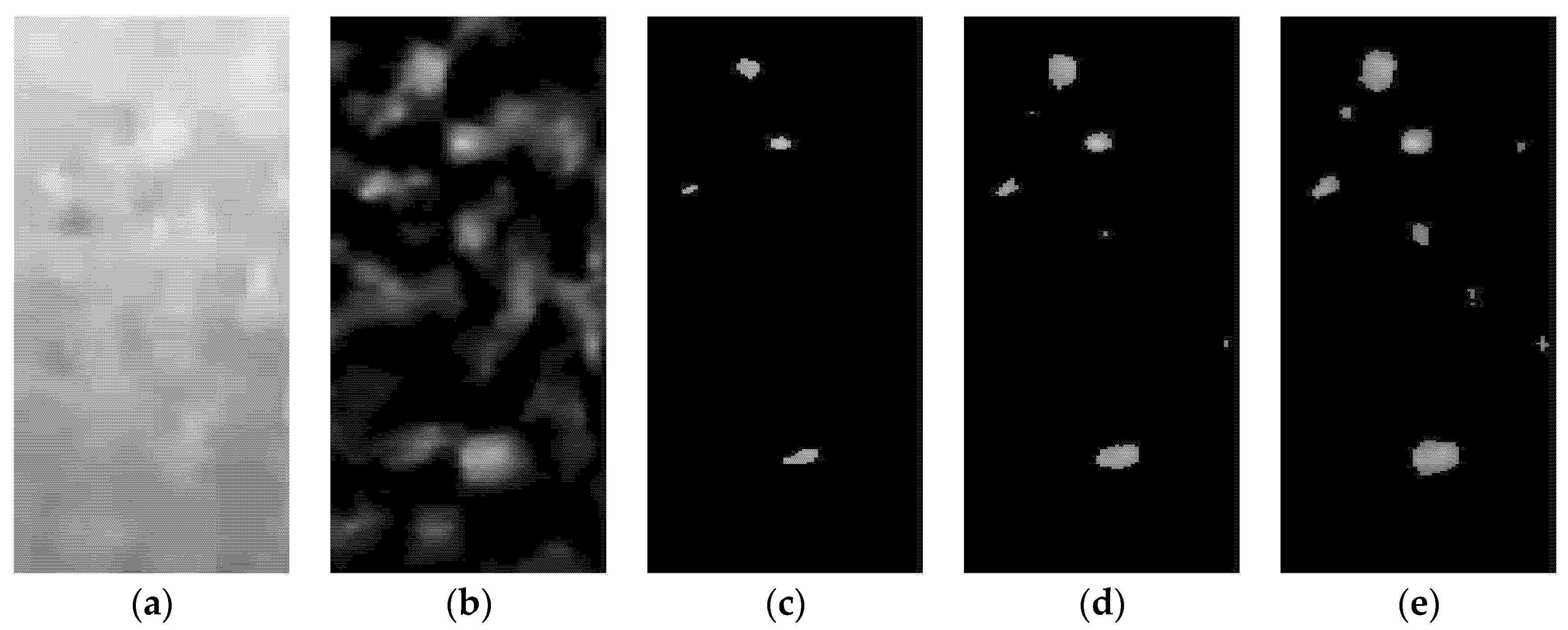
24] (see
Supplementary Materials). In order to improve the sharpness of the video frames, Free-LSPIV employs application of the Gaussian blur filter, image subtraction, conversion to greyscale, and contrast adjustment; the latter involves turning off all the pixels with brightness lower than a threshold. To define this threshold, the contrast adjustment parameter is employed. The threshold is the product of this parameter by the maximum brightness value of the processed area. A parameter value equal to 1 means all pixels, except for the brightest, are turned off. A value equal to 0 means none of the pixels are turned off. Any value between 0.3 and 0.9 can be considered a plausible value (see
Figure A1 in
Appendix A).
Free-LSPIV uses fast normalized cross-correlation [
25,
26] between the IA (taken from a video frame) and the search area (taken from the next video frame). The location of the maximum value in the resulting correlation matrix gives the most probable displacement between the two frames. In some cases, the maximum value of this matrix may correspond to irrelevant particles. For example, in the case where IA contains only one particle just about to exit the IA with the flow, and the search area contains only one particle just entering. To filter out these cases, a parameter that defines the minimum acceptable cross-correlation is used. The location of the maximum value in the correlation matrix is considered valid displacement only if this value is greater than the minimum acceptable cross-correlation. From a mathematical perspective, this parameter value can be between –1 and 1, but for this application, it is more reasonable to select a value for the parameter between 0.3 (a value equal to 0 would not filter noise) and 0.9 (a value equal to 1 would mean the IA remains unchanged between successive frames).
Therefore, any Free-LSPIV application requires defining three parameters: the contrast adjustment, the minimum acceptable cross-correlation, and the IA size. The search area size can be obtained by appropriately augmenting the IA size to ensure the capacity to capture any possible particle displacement of the studied flow conditions.
The influence of the aforementioned parameters on the accuracy of Free-LSPIV was studied by employing Monte Carlo simulations. This included multiple runs of Free-LSPIV with different sets of parameter values. It should be noted that the methodology is not specific to Free-LSPIV and can be applied to any image velocimetry method that requires a definition of IA and other parameters. In fact, Monte Carlo simulations were employed for a similar purpose by Keane and Adrian [
27,
28].
The standard approach in Monte Carlo simulations is to generate random numbers using the triangular distribution [
29,
30] for obtaining the values of the parameters. Since the CPU time required for the execution of image velocimetry algorithms is considerable, it is not feasible to employ a large number of iterations. For this reason, and to ensure that the spread of the values produced by the random number generator is as wide as possible (but always inside the prescribed limits), Equation (2) was used to produce the random numbers:
where
xi is the
ith value from the total
n values produced by the random number generator,
ΦTR is the inverse cumulative of the triangular distribution function, and,
a,
b, and
c (with
a <
c <
b) are the parameters of the triangular distribution.
The distribution parameters a, b, and c of the triangular distribution correspond to the plausible minimum, plausible maximum, and most likely values of the variable, respectively. The (a, b, c) values for the three studied parameters, i.e., the contrast adjustment parameter, the minimum acceptable cross-correlation, and the IA size were (0.3, 0.9, 0.7), (0.3, 0.9, 0.6), and (½L, 2L, L), respectively. In the last triplet, L is the mean IA side length in pixels (IAs are squares) of the n different IAs that were employed in the Monte Carlo simulations. Using Equation (2), n values were produced for each one of the three Free-LSPIV parameters. Then n3 sets of parameter values were formed employing the Cartesian product on the three sets of which each one has n generated parameter values. Free-LSPIV was run for each one of these n3 sets. This produced n3 velocity profiles along the cross-section from which the lower limit of the 90% confidence interval, the mean value, and the upper limit were derived.
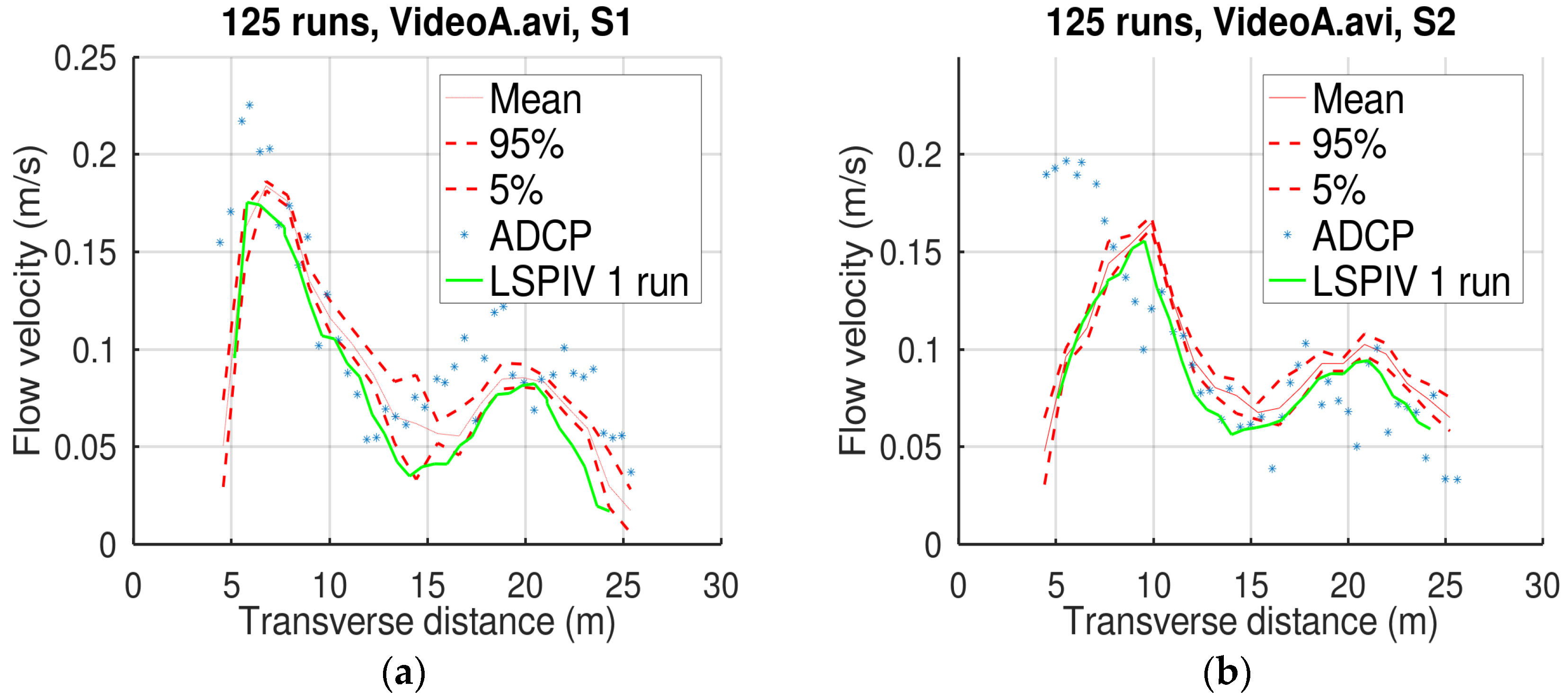
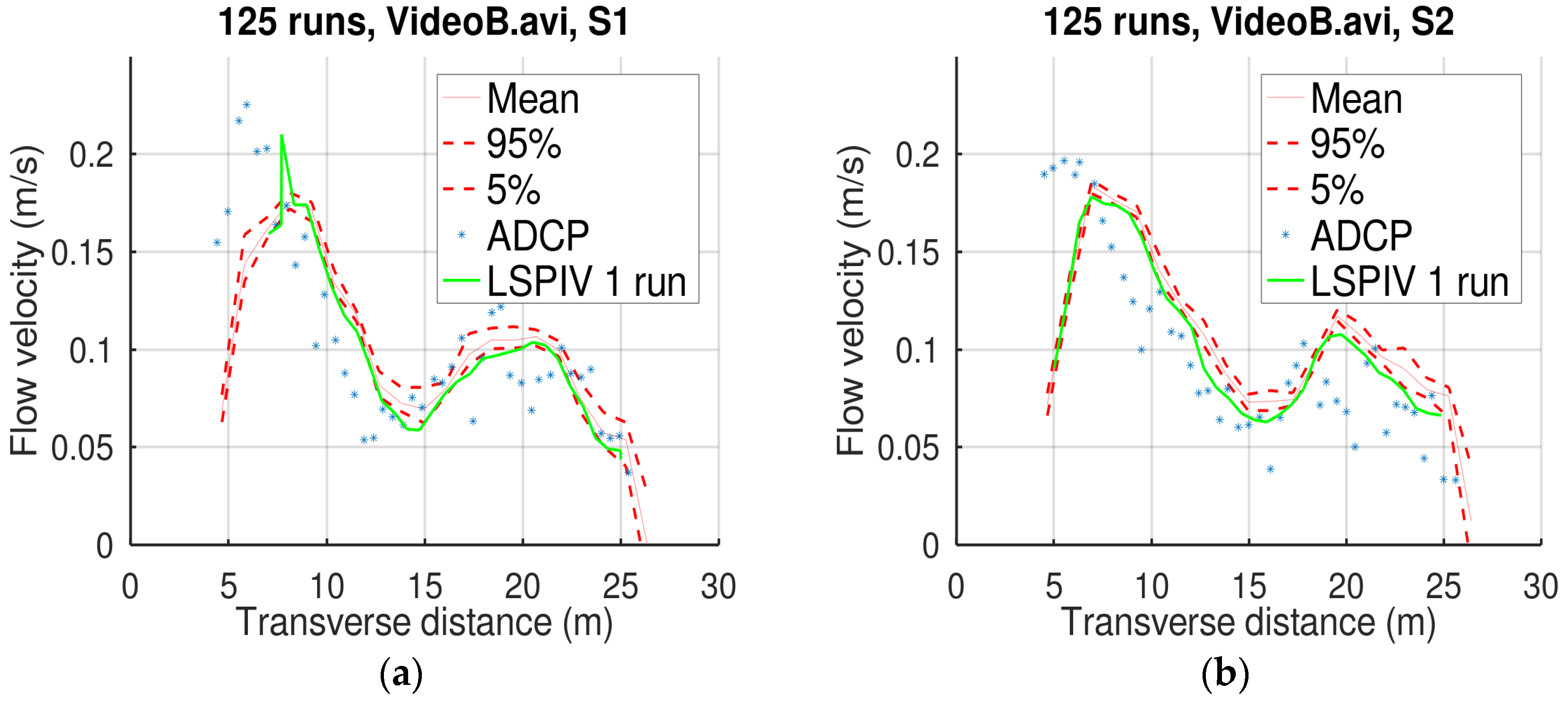
The video and measurements used in this study were obtained from the data made publicly available by Pearce et al. [
20]. Pearce et al. recorded two videos, Video A and Video B, of the flow of the Kolubara River near the city of Obrenovac in Central Serbia. The resolution of the videos is 3696 × 4994, their length is 25 and 21 s, respectively, and the frame rate is 23 fps. They also performed ADCP measurements along two cross-sections, named S1 and S2. The two videos combined with the two cross-sections resulted in four different datasets, which were used for testing the suggested methodology.
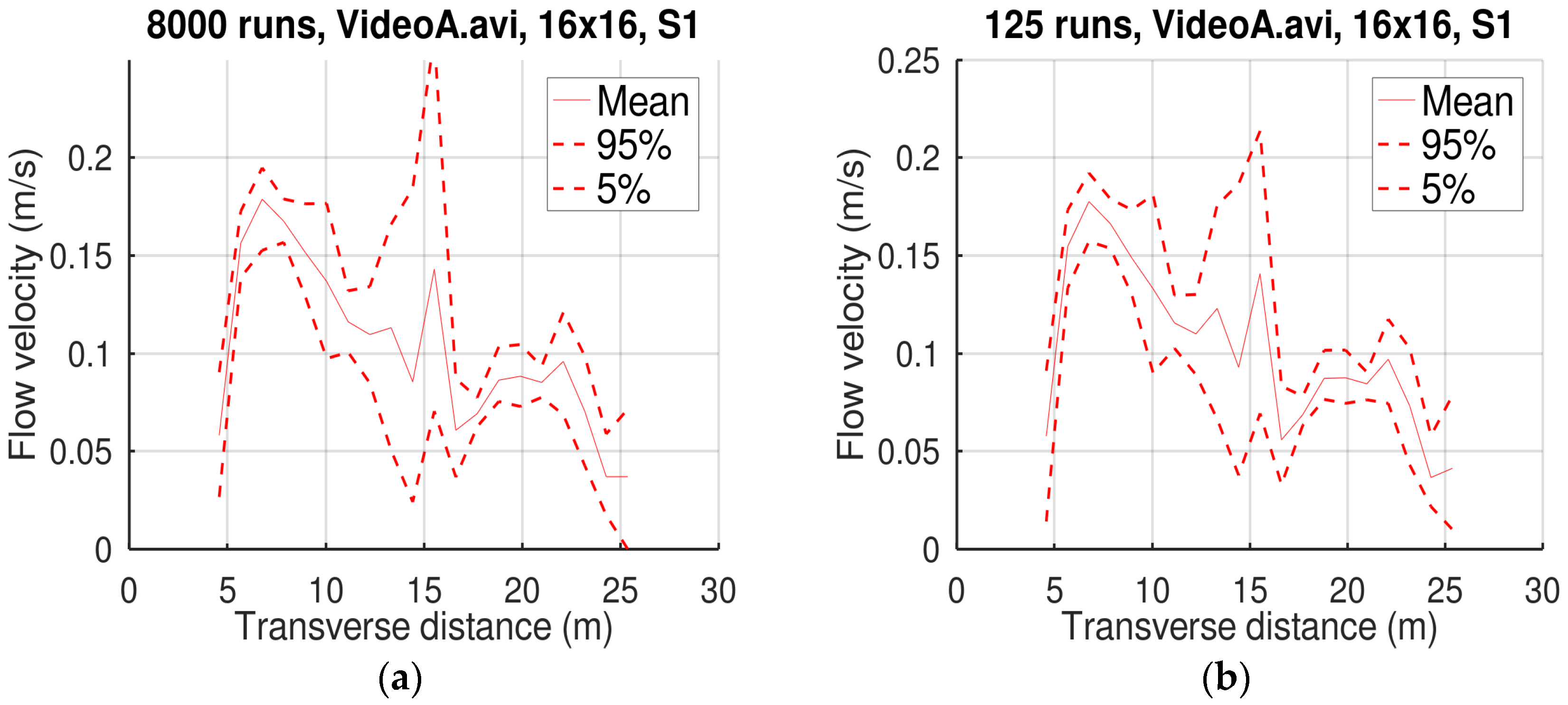
As mentioned previously, the CPU time of the image velocimetry methods is considerable. For this reason, it was initially investigated whether Equation (2) helps to obtain reliable estimations of the statistical profiles (lower limit, mean, and upper limit) with a limited number of iterations. For this reason, Monte Carlo simulations were applied to cross-section S1 of Video A with n = 20 (203 runs) and n = 5 (53 runs). The results of these simulations were compared to evaluate the sufficiency of a limited number of simulations to successfully capture the influence of uncertainty of parameters on the results.
Afterward, the information provided by the width of the zone between the lower and the upper limit of the 90% confidence interval was examined. It should be noted that this width represents only the uncertainty attributed to the parameters. The errors due to the intrinsic limitations of the image velocimetry methods were not captured. For example, in Pearce et al.’s study [
20], all tested methods failed to correctly estimate the velocities near the right bank ([
20], Figure 8) because surface features were sparse. This error cannot be avoided regardless of the selected parameter values.
It should be noted that
L is the only parameter of the suggested method. It defines the IA sizes, which, for the given (
a,
b,
c) values, range from
L/2 ×
L/2 to 2
L × 2
L. A similar choice of multiple IA sizes is employed in PIVlab. According to Thielicke [
31], PIVlab’s accuracy is improved by employing three passes with IA sizes that are consecutive multiples of two. The optimum value of
L depends on the density of the features captured by the video (more specifically the image density, i.e., the mean number of particle image pairs per interrogation volume [
32]), the flow conditions, and the camera position. An empirical rule was derived in order to select the optimum
L based on the confidence interval width. For this reason, the influence of
L on the confidence interval width and the relation of the confidence interval width to the model accuracy were investigated. To do so, various
L values were selected manually and then Monte Carlo simulations were executed (see
Figure 1). After a series of Monte Carlo simulations with different
L values, a group of results was compiled comprising the manually selected
L value, the corresponding confidence interval width, and the accuracy of the mean profile compared to the ADCP velocity profile.
As mentioned previously, the multi-pass approach has been suggested to improve the accuracy of the particle image velocimetry methods. In this approach, information exchange takes place between successive passes by using the results of a preceding pass to offset the IA of the following pass [
22]. This indicates that blending the information obtained with various IAs is advantageous. For this reason, the mean velocity profile produced by Monte Carlo simulations, which is an amalgamation of all simulation results, may be advantageous, in the same sense the multi-pass approach is advantageous over single runs.
4. Discussion
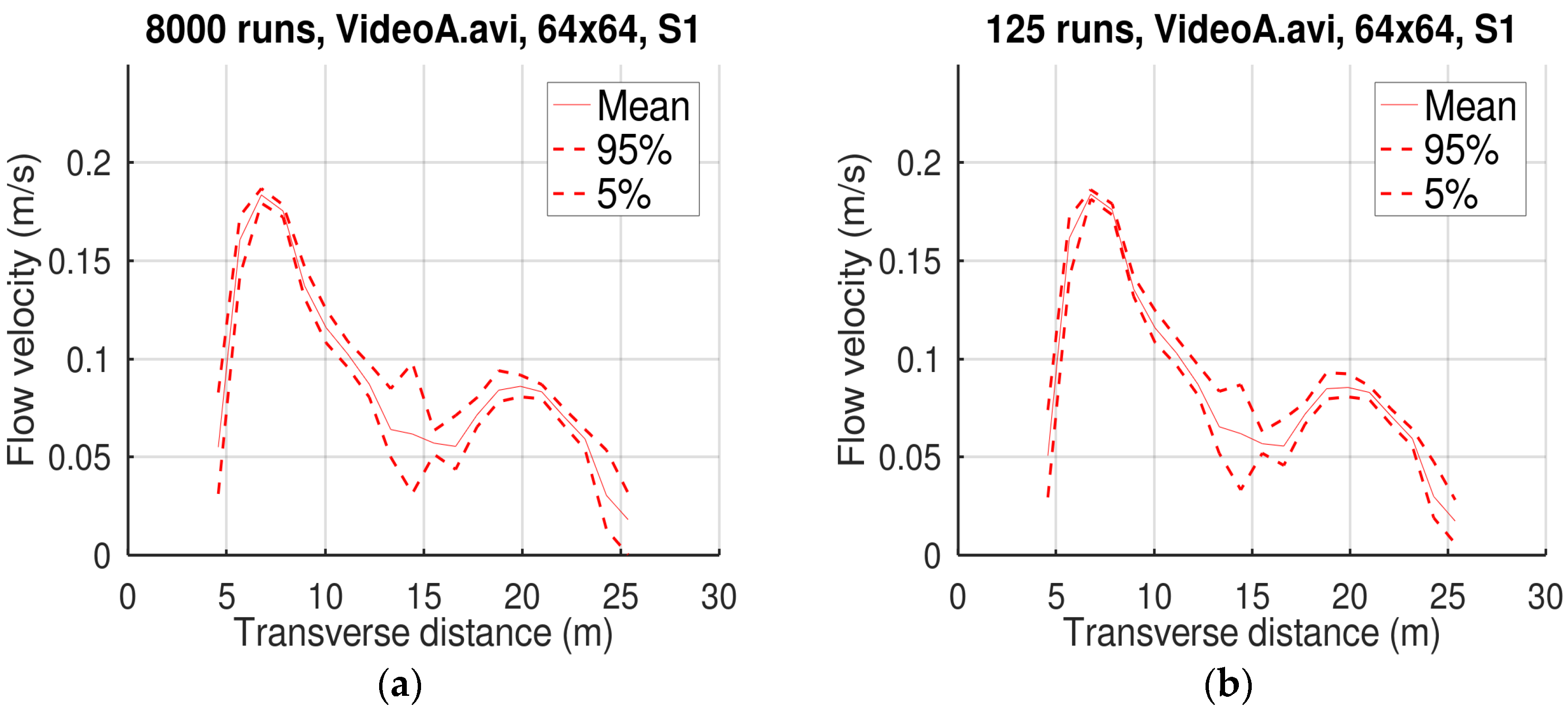
The comparisons of the Monte Carlo results with 20
3 and 5
3 runs displayed in
Figure 2,
Figure 3 and
Figure 4 and in
Table 2 suggest that the use of Equation (2) for generating random numbers helped reliably estimate the statistical profiles even with a limited number of simulations. This is very important taking into account the considerable CPU time required by image velocimetry methods.
Regarding the selection of the IA size, this remains a challenge despite techniques like the multi-pass approach or the Monte Carlo simulations used in this study. In both approaches, a mean IA size is defined and simulations with a range of IA sizes surrounding the mean value are performed.
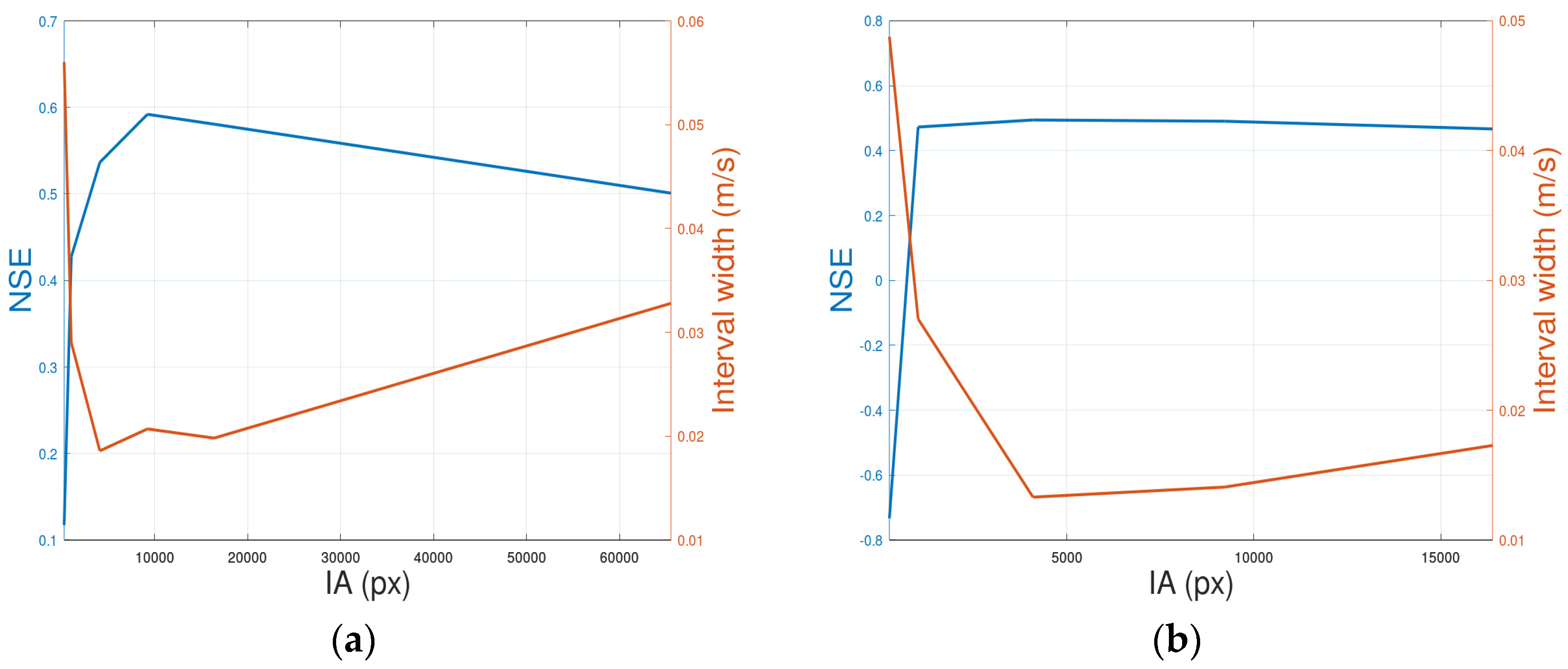
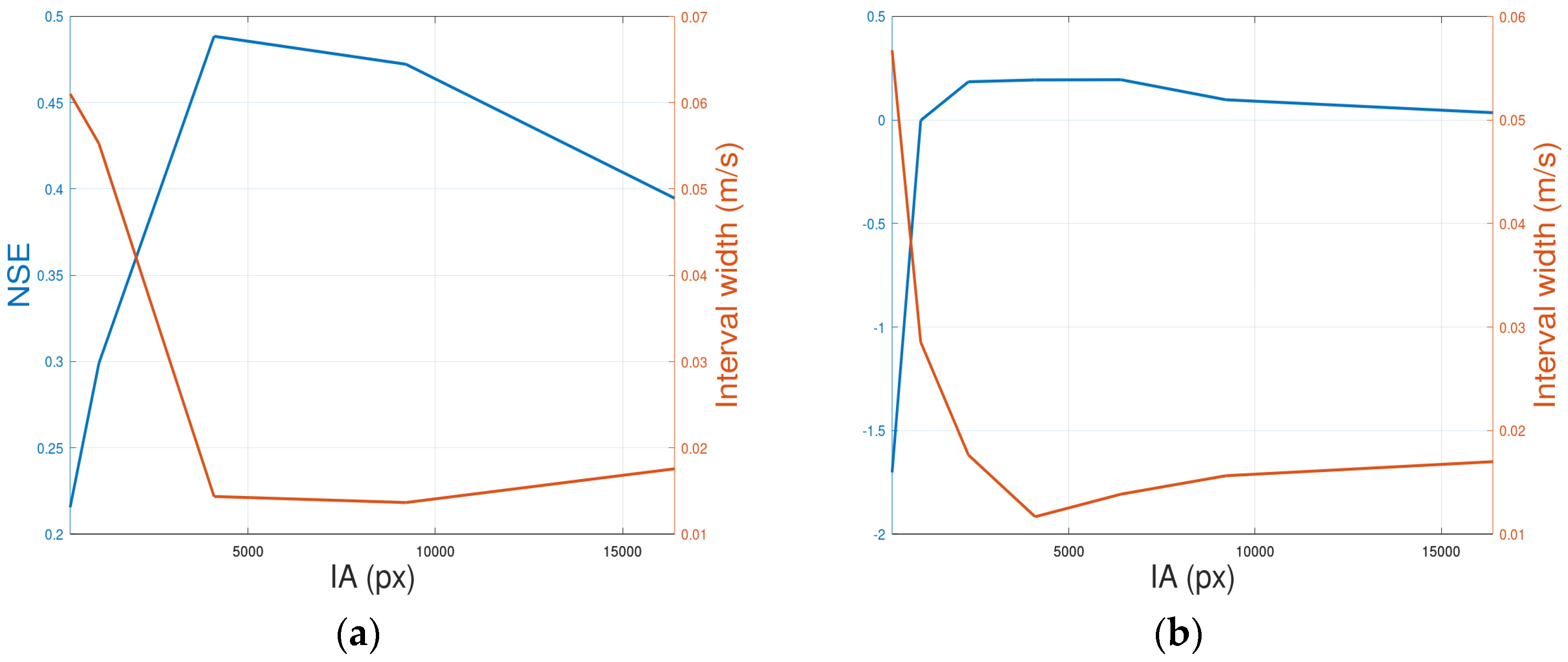
Figure 5 and
Figure 6 demonstrate the importance of the mean value. In all cases, the accuracy of the estimated velocities initially increased with the IA size, and then either stabilized or deteriorated. This is compatible with the findings of other researchers [
21] who observed that larger IA sizes allow to improve the signal-to-noise ratio, but at the same time result in lower cross-correlation peak values, which reduces the confidence on the detected velocity vectors. Additionally, larger IA sizes reduce the effective resolution [
33], which has a negative impact on the accuracy. Therefore, it is crucial to select the optimal IA size for each application.
Figure 5 and
Figure 6 give an interesting hint. The IA size that achieved the best accuracy was close to the IA size that achieved the narrowest confidence interval. Therefore, with a series of Monte Carlo simulations with various mean IA sizes (
Figure 1), one can obtain an indication of the optimum IA size.
The rest of the Free-LSPIV parameters do not vary greatly over different applications (always ranging between 0.3 and 0.9). These parameters do not require any handling. In single-run applications, one needs to subjectively select a value for these parameters. However, when Monte Carlo simulations are employed, there is no need for the selection of a specific value. The influence of uncertainty regarding the values of these parameters on the results is quantified by the confidence interval.
Figure 7 and
Figure 8 and
Table 3 suggest that the mean profile of the Monte Carlo simulations achieved better accuracy than the LSPIV with a single run. The suggested methodology exhibited a relative bias of 13.66% in this specific application (Kolubara River). The LSPIV with a single run exhibited a relative bias of −21.63% for the specific PIVlab parameters selected by Pearce et al. for this application. If Monte Carlo simulations were used with PIVlab, PIVlab could have exhibited lower bias that may be lower than that of Free-LSPIV.
Finally, a long-term benefit of using Monte Carlo simulations is the full exploration of the peculiarities of the employed image velocimetry algorithm. For example, if the mean profile consistently overestimates or underestimates the surface velocities in many different applications, then this would be an indication that the algorithm introduces a systematic bias. This would allow to fine-tune the algorithm to remove this bias or introduce correction coefficients.
The following steps are suggested to improve the accuracy of an image velocimetry method with Monte Carlo simulations:
Identify the parameters of the method and their plausible maximum/minimum and most likely values.
Employ Equation (2) to generate sets of random values for the parameters. A small number of values (e.g., n = 5) for each parameter is sufficient.
Start with a low value for mean IA size (e.g., L × L = 16 × 16 pixels) and produce a small number (e.g., n = 5) of IA sizes employing Equation (2) with (a, b, c) = (½L, 2L, L).
Run Monte Carlo simulations and obtain the mean and the lower and upper limits.
Increase L by a factor between 1 and 2. The confidence interval width will initially decrease with L. When the confidence interval stops decreasing with L, go to the next step, otherwise repeat steps 3 and 4.
Identify the Monte Carlo simulation with the lowest confidence interval width and use the mean velocity profile of this simulation as the best estimation of the surface velocities.
It should be noted that the confidence interval produced by the Monte Carlo simulations, as described above, does not consider the errors due to the intrinsic limitations of the image velocimetry methods. This type of error is currently under investigation. For example, Dal Sasso et al. [
34] introduced a metric to evaluate the density and characteristics of the features on the surface of flowing water, which helps obtain a prior estimation of the error of the image velocimetry method. Perks et al. [
35] recently made available a range of datasets that were compiled from across six countries. These data could serve as the test bed for deriving a method that would estimate the overall error from both sources.
Finally, it should be noted that repeated Monte Carlo applications with different
L values, instead of a single application of Monte Carlo with a very wide range of IA sizes, are recommended for various reasons. First, a very wide range would include large IA size values to Monte Carlo simulations, which, if far from the optimum
L value, would result in an unnecessary increase of CPU time (see
Table 1). Second, a low
n value with a large parameter space would result in a poor representation of this space by the
n generated random values. Finally, the confidence interval would be much wider than that of the previously described steps.


