Abstract
To properly manage the groundwater resources, it is necessary to analyze the impact of groundwater withdrawal on the groundwater level. In this study, a Long Short-Term Memory (LSTM) network was used to evaluate the groundwater level prediction performance and analyze the impact of the change in the amount of groundwater withdrawal from the pumping wells on the change in the groundwater level in the nearby monitoring wells located in Jeju Island, Korea. The Nash–Sutcliffe efficiency between the observed and simulated groundwater level was over 0.97. Therefore, the groundwater prediction performance of LSTM was remarkably high. If the groundwater level is simulated on the assumption that the future withdrawal amount is reduced by 1/3 of the current groundwater withdrawal, the range of the maximum rise of the groundwater level would be 0.06–0.13 m compared to the current condition. In addition, assuming that no groundwater is taken, the range of the maximum increase in the groundwater level would be 0.11–0.38 m more than the current condition. Therefore, the effect of groundwater withdrawal on the groundwater level in this area was exceedingly small. The method and results can be used to develop new groundwater withdrawal sources for the redistribution of groundwater withdrawals.
1. Introduction
Groundwater is an important water resource that can be used in tandem with surface water, and research on groundwater is especially important in island areas because it comprises most of the water for used living and agriculture. On Jeju Island in Korea, groundwater is an exceedingly important water resource that accounts for about 80% of the total water resource use. Therefore, research on the effects of withdrawals on groundwater levels is especially important for its continuous and stable use. The variability in the groundwater level is influenced by seasonal variations in precipitation, groundwater withdrawals, and river water level changes [1]. Jeju Island is a region with a high amount of precipitation, but most of its rivers are dry streams because of the soil’s high water permeability, so the water level of the rivers has a negligible impact on the groundwater level. Therefore, to provide information for the proper management of Jeju Island’s groundwater resources, it is necessary to analyze the effects of precipitation and withdrawals on the groundwater level.
Excessive withdrawals from a specific pumping well in an island region creates problems for sustainable groundwater yields, such as rapid decreases in groundwater levels and seawater intrusions [2]. To solve these problems, Oki [2,3] conducted a study to reduce groundwater level decreases by redistributing withdrawals using a numerical model and various withdrawal scenarios. As a result, groundwater level increased as the withdrawal amount decreased. Therefore, a direct relationship between the thickness of the aquifer and the groundwater withdrawal reduction amount as well as the effect of the withdrawal redistribution were confirmed. To analyze the impact of groundwater withdrawals using a numerical model, spatial data with various physical properties such as detailed land use maps and geological maps for the study area are required; however, in reality, these data are often insufficient. If an explicit model-driven approach cannot be used because of the difficulty of collecting these heterogeneous data, the explicit model-driven approach can be supplemented through an implicit data-driven approach, i.e., machine learning [4,5].
Various machine learning models can be used for groundwater analysis, from the traditional Artificial Neural Network (ANN) and Support Vector Machine (SVM) to novel deep learning methods such as Long Short-Term Memory (LSTM). ANN has been widely used in various research fields as a representative machine learning method [6]. However, ANN cannot learn long-term data (long-term dependency problem) [7,8], so the appropriate prediction period is not as long as 1 to 3 time steps (e.g., one- to three-day prediction) [9]. The SVM proposed by Vapnik [10] is more predictive than ANN [11] and is a data-driven model widely used in the field of machine learning [12]. A previous study analyzed the effect of changes in groundwater withdrawals on the extent of seawater intrusion into coastal aquifers using SVM [13], but SVM reportedly demonstrated a lower predictive capacity than LSTM [14].
The purpose of this study was to evaluate the groundwater prediction performance of the LSTM network [15], which comprises a novel recurrent neural network (RNN) that can remember input data over a long period [16] by solving the long-term dependency problem [17] of existing RNNs. Moreover, we analyzed the effects of changes in withdrawals from pumping wells on changes in the groundwater level of monitoring wells using LSTM to reduce decreases in groundwater supplies. LSTM is a deep learning model suitable for learning continuous data, such as time series data, and has recently been used in various groundwater analysis studies [18,19,20,21,22,23,24,25]. The details of the LSTM are described in Section 2.2.
2. Materials and Methods
2.1. Study Area and Data
The study area comprised of two groundwater monitoring well points located in the central mountainous region of Pyoseon watershed in the southeast portion of Jeju Island (Figure 1). This study used daily precipitation data from the Seongpanak and Gyorae rainfall stations in the vicinity of groundwater monitoring wells, daily groundwater withdrawal data from two groundwater pumping wells (pumping well 1 (PW1) and pumping well 2 (PW2)), and daily groundwater level data from two groundwater monitoring wells (monitoring well 1 (MW1) and monitoring well 2 (MW2)) (Table 1). Data from the Seongpanak rainfall station (automatic weather station), which is operated by the Korea Meteorological Administration (http://www.weather.go.kr/), and Gyorae rainfall station, which is operated by the Jeju Island Disaster and Safety Countermeasures Headquarters (http://bangjae.jeju119.go.kr/), are provided online. The withdrawal data of the pumping wells and the groundwater level data of the monitoring wells were observed and operated by the Jeju Province Development Corporation. The locations of rainfall stations, groundwater pumping wells, and groundwater monitoring wells in the study area are shown in a diagram (Figure 1). Precipitation at the rainfall stations and groundwater level in the monitoring wells are shown in Figure 2 and Figure 3, respectively. In Figure 2, the precipitation at the Seongpanak rainfall station is greater than that at the Gyorae rainfall station. Accordingly, the Seongpanak rainfall station (El. 763 m, Figure 1) is located at a higher elevation than the Gyorae rainfall station (El. 400 m, Figure 1), and the former is more affected by the orographic lift effect than the latter, resulting in greater precipitation. In Figure 3, the degrees in groundwater level variation of MW1 and MW2 are similar; however, the groundwater level of MW1 is higher than that of MW2.
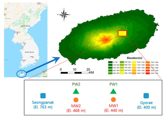
Figure 1.
Schematic of the positions of rainfall stations, groundwater pumping wells, and groundwater monitoring wells.

Table 1.
Data period of rainfall stations, groundwater pumping wells, and groundwater monitoring wells.
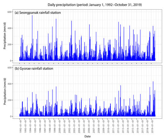
Figure 2.
Comparison of daily precipitation in Seongpanak and Gyorae rainfall stations.
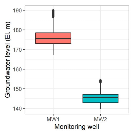
Figure 3.
Boxplot for the variability of groundwater level in monitoring wells.
2.2. Long Short-Term Memory (LSTM)
Long Short-Term Memory [15] is a modification of the RNN developed to solve the vanishing gradient problem [17], which makes it impossible for RNN to learn long-term dependencies. LSTM uses a conveyor belt (carry track, Figure 4) placed parallel to the sequence being processed so that the information from the sequence can be transported to the carry track at any point in time and then transported to a later time to be reused when needed. The information is stored in a carry track for later use, and therefore, there is no problem if the old signal gradually disappears during the calculation process [26]. LSTM was developed to remember long-term information and has a recurrent structure similar to the existing standard RNN, but the former differs from the latter in that it learns long-term information using four unique transformations. First, the output of the cell for time t () is calculated as follows:
where is the input data for time t;
is the state for time t, which is the state of output for time t−1; is the carry value for time t; , , and are the weight matrices of , , and , respectively, for output calculation; and is the dot product. The weights are the parameters of the LSTM and play the most important role in calculating the output. is the bias followed by the weight matrices, and is the activation function using the sigmoid () function and function.
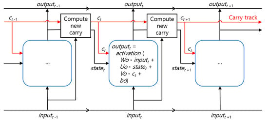
Figure 4.
LSTM architecture. Reproduced from Chollet and Allaire [26].
The carry value is updated using three separate transformations, and all three individual transformations take the form of a simple RNN cell. The three individual transformations are as follows, all of which have unique weight (parameter) matrices.
where is the newly added information (ranging from 0 to 1) through a sigmoid function (), is the deleted information (ranging from 0 to 1) through a sigmoid function, and is the importance of information (ranging from −1 to 1) through a function. LSTM multiplies and to obtain new information, and are multiplied to remove irrelevant carry information, and finally and are added to obtain a new carry value. Therefore, LSTM uses the carry track to modulate the next output and next state [26].
Figure 5 shows LSTM’s supervised learning procedure. The data input to the layer of the LSTM is converted by weights that are parameters of the layer. The groundwater level simulated by LSTM is compared with the observed groundwater level using the objective function (here loss function), and the weights are adjusted (updated) through the optimizer until the simulated groundwater level is closest to the observed groundwater level (i.e., until loss is minimized). The process of gradually adjusting the weights is called training, and LSTM is learned through training. Therefore, the weights contain the learned information, and the optimizer uses the backpropagation algorithm. In this study, LSTM included in the Keras package [27], which is an R language-based deep learning framework, was used.
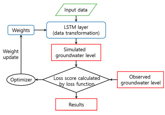
Figure 5.
LSTM modeling process. Reproduced from Chollet and Allaire [26].
2.3. Method
First, this study predicted the groundwater level for one day ahead via the LSTM for groundwater monitoring wells and evaluated the model’s predictive performance. The reason for selecting the one day ahead prediction was that the LSTM had the highest predictive performance with this prediction type, so the calibrated LSTM parameters best reflected the variation characteristics of the observed groundwater level. In addition, the reason that periods of more than one day ahead were not predicted is that the purpose of this study is not to predict long term future groundwater levels via LSTM, but to analyze the effect of changes in withdrawals on variations in groundwater levels. To prevent overfitting of LSTM parameters with respect to training period data among the entire period of observation data, the estimated parameters were validated using validation period data through a callback method. In addition, test periods were used to evaluate the predictive performance of the LSTM. Training, validation, and test periods were deemed independent, and each period is shown in Table 2.

Table 2.
Training, validation, and test periods for LSTM modeling.
For the training of LSTM, the values of hyper-parameters required for model building must be set, and there are no clear instructions on how to set them [26]. In this study, hyper-parameters were set as shown in Table 3. The n_timesteps denote the number of prediction days, and as described above, the number of prediction days was set to 1. The n_units represent the number of hidden units in the LSTM layer, i.e., the dimension of the layer, which denotes the degree of freedom a neural network can have for learning [26]. The larger the value of n_units, the more complicated the data that can be learned; thus, the convergence of the objective function values is faster, but the calculation time is longer and overfitting problems for training data can occur. In this study, dropout and callback methods were used to prevent overfitting, so sufficient n_units were used. As a result of trial and error, the n_units amount was set to 100. LSTM does not process the entire dataset during the training period at one time, thus dividing it into a small sample group, or a mini batch, to process the dataset during the training period. The batch_size refers to the number of data points in the mini batch to be processed once in the training dataset for training of LSTM. In this study, this amount was set to 50 considering the characteristics of daily training data and the duration of training data. A dropout was used to prevent overfitting during the training process by randomly removing multiple output features of the layer [28]; generally, dropouts use a value between 0.2 and 0.5. In this study, both the dropout and recurrent_dropout were set to 0.5 as a result of trial and error. For the optimization algorithm, Adam [29] was used, which is widely used for optimization in recent deep learning fields [30], and the mean absolute error was used for the objective function. Adam optimizer uses the stochastic gradient decent procedure. For the learning_rate, which denotes the learning rate of the Adam optimizer, the default value of 0.001 was used. For the optimization process, one iteration for the entire training dataset is called an epoch, and the n_epochs, which defines the maximum number of iterations, was set to 50 as a result of trial and error. The callback is a method of early termination when simulation results are no longer improved by repeating training as much as an arbitrarily selected threshold value. The patience, which is a hyper-parameter for the callback method, denotes this threshold, and the patience was set to 10 as a result of trial and error.

Table 3.
Setting values of hyper-parameters in LSTM.
The Nash–Sutcliffe efficiency (NSE) [31] and root mean square error (RMSE), which are widely used in the field of hydrology, were used to evaluate the simulation performance of LSTM by comparing the simulated groundwater level with the observed groundwater level. The NSE provides overall information on simulation results [32], and RMSE indicates how closely simulated values match observed values [30]. The NSE and RMSE are defined as follows:
where n is the number of time steps, and are the observed and simulated groundwater levels in time step i (daily here), respectively, and is the average value of the observed groundwater level. The range of NSE is −∞ to 1; 1 means that the simulated values exactly match the observed values, and 0 means that the simulated values are equal to the mean of the observed values. An RMSE of 0 means that the simulated values exactly match the observed values.
Second, the estimated parameter values and groundwater withdrawal scenarios were used to calculate the groundwater level of the monitoring wells and to analyze the effect of changes in withdrawals on the groundwater level variability. Withdrawal scenarios were set based on the assumption that a new groundwater pumping well will be constructed in the future to reduce the decrease in the groundwater level in the monitoring wells caused by the withdrawals from pumping wells. We assumed that the current withdrawal rate for both PW1 and PW2 was 2300 m3/d, and for the future scenario, we assumed that PW1 and PW2 would take as much as 2/3 of the current withdrawal rate considering the development of a new pumping well. Therefore, withdrawal Scenario1 is a case where no groundwater is taken, Scenario2 is a case where the groundwater of 1533 m3/d (2/3 of 2300 m3/d) is taken daily, and Scenario3 is a case where the groundwater of 2300 m3/d is taken daily. This study used these three withdrawal scenarios to analyze the effect of the amount of withdrawal reduction on the degree of groundwater level increase and the linearity or nonlinearity between the amount of withdrawal reduction and the groundwater level increase. In addition, this study analyzed the limitations of LSTM, a data-driven approach, for modeling groundwater levels.
3. Results
3.1. Analysis of the Prediction Performance of LSTM
Figure 6 and Figure 7 show the one-day prediction performance of the groundwater level by LSTM for the training, validation, and test periods of MW1 and MW2, respectively. In the figures, the horizontal axis represents the observed groundwater level, the vertical axis represents the simulated groundwater level, and the red dashed line represents the one-to-one line.
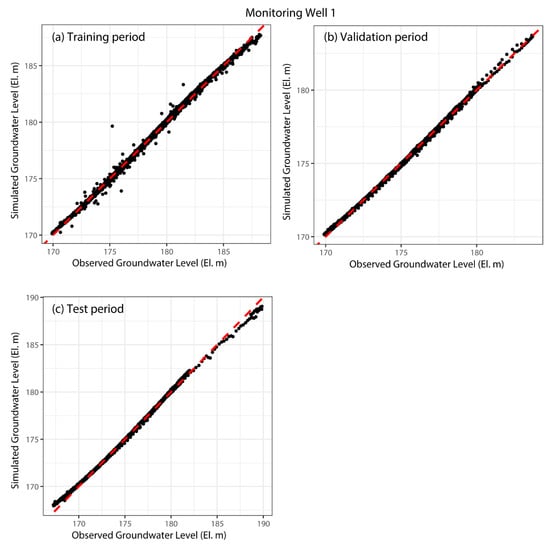
Figure 6.
Simulated and observed groundwater levels for monitoring well 1.
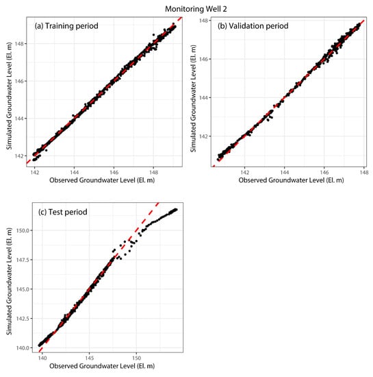
Figure 7.
Simulated and observed groundwater levels for monitoring well 2.
In the case of MW1 with a relatively long data period (approximately 19 years), the one-day prediction performances of groundwater level by LSTM for the training, validation, and test periods were exceedingly high, with NSE values of 0.99 or higher (Figure 6, Table 4). This was because the training period required for model calibration was sufficiently long (approximately 13 years), and the training period contained enough information to predict the groundwater level during the validation and test periods.

Table 4.
Modeling performance of LSTM for the one-day groundwater level prediction.
In the case of MW2 with a relatively short data period (approximately 6 years), the one-day groundwater level prediction performances by LSTM for training and validation periods were also high, with NSE values of 0.99 or higher (Figure 7, Table 4). However, the prediction performance for the test period was relatively low, with an NSE of 0.976, and the one-day prediction performance for relatively high groundwater levels above 150 m was relatively low (Figure 7, Table 4). This was because the training period required for model calibration was relatively short (approximately 2 years and 6 months), so the information designated for predicting the relatively high observed groundwater level included in the test period was not sufficient for the training period.
Although the groundwater level prediction performance during the test period of MW2 was relatively lower than that of MW1, the NSE was 0.97 or higher and the RMSE was 0.5 or lower, showing a sufficiently high prediction performance. In addition, the results of MW1 also showed a high prediction performance. Therefore, LSTM’s ability to predict groundwater levels was sufficiently high. This study analyzed the effect of changes in groundwater withdrawal on variations in groundwater level using estimated parameter values, as shown in Section 3.2.
3.2. Analysis of the Effect of Changes in Groundwater Withdrawals on the Variations in Groundwater Levels
Figure 8 shows the representative section (1–30 September 2018) of the simulated groundwater level variations according to the change in the withdrawal amounts for MW1 and MW2. As expected, the groundwater level was highest for Scenario1 with no withdrawal, followed by Scenario2 (withdrawal of 1533 m3/d) and Scenario3 (withdrawal of 2300 m3/d).
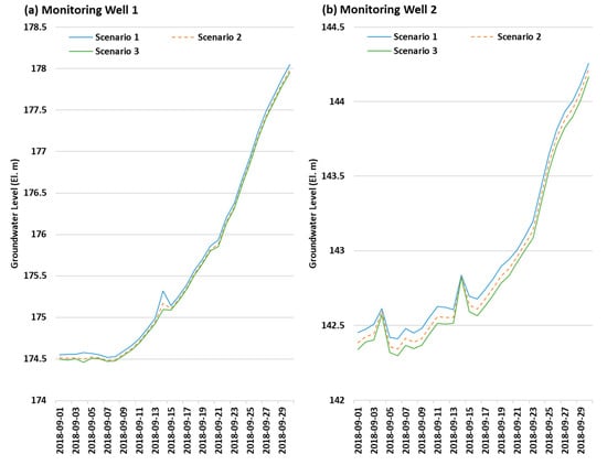
Figure 8.
Groundwater levels predicted using LSTM and groundwater withdrawal scenarios for MW1 and MW2.
Table 5 shows the differences between the simulated groundwater levels by withdrawal scenarios for the entire data period for each monitoring well. In the case of MW1, when the withdrawal amount was reduced by 1/3 through taking 1533 m3/d (Scenario2) from the withdrawal of 2300 m3/d (Scenario3), the increase in groundwater level was estimated to be up to 0.13 m and an average of 0.03 m. In addition, when the groundwater was not taken (Scenario1), the groundwater level rose to 0.38 m and an average of 0.09 m compared to the case where 2300 m3/d was withdrawn (Scenario3). Therefore, the increase in groundwater level between Scenario1 and Scenario3 was estimated to be approximately three times larger than that for Scenario2 and Scenario3. This linear relationship between the change in the withdrawal amount and the variation in the groundwater level indicates that the permeability of the subsurface geology and the groundwater yield around MW1 are high, so the groundwater level will increase as the withdrawal amount decreases. In addition, the maximum difference in groundwater level between Scenario1 and Scenario3 was 0.38 m, which means that in this area, the effect of the withdrawal on the groundwater level was small.

Table 5.
Differences between the simulated groundwater levels in groundwater withdrawal scenarios for the entire data period.
In the case of MW2, when the withdrawal amount was reduced by 1/3 from 2300 m3/d (Scenario2–Scenario3), the increase in groundwater level was estimated to be 0.06 m at the maximum and 0.05 m on average. In addition, when the groundwater was not taken (Scenario1), the groundwater level increased to 0.11 m and an average of 0.09 m compared to the case where the groundwater was taken at 2300 m3/d (Scenario3). Therefore, the increase in groundwater level between Scenario1 and Scenario3 was estimated to be twice that for Scenario2 and Scenario3. Therefore, given the uneven differences in reduction rates and groundwater level increases between scenarios, the change in groundwater withdrawal had a nonlinear relationship with the variation in groundwater level. This means that the geological properties around MW2 are different from those of MW1, and therefore, there is a difference in permeability and groundwater yield. In addition, in the case of MW2, the maximum difference in groundwater level between Scenario1 and Scenario3 was only 0.11 m, and hence, the effect of the withdrawal rate on the groundwater level in this area was exceedingly small.
However, in the case of MW2, the periods when the groundwater level simulated by Scenario1 was lower than the groundwater levels simulated by Scenario2 and Scenario3 (inversion phenomenon of simulated groundwater level) accounted for approximately 2.5% of the entire data period (Figure 9). Therefore, LSTM had limitations in its ability to simulate the groundwater level for the groundwater withdrawal scenarios. However, the period in which the inversion of the simulated groundwater level occurred was short, at approximately 2.5% of the entire simulation period. Hence, the effect of this inversion on calculating the difference in groundwater level for Scenario1–Scenario3 of MW2 was minor. Therefore, the statistical values for Scenario1–Scenario3 of MW2 in Table 5 represent the results of calculating the difference in groundwater level using simulated groundwater level data, excluding the inversion period.
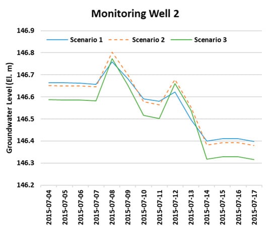
Figure 9.
Inversion of simulated groundwater levels using the groundwater withdrawal scenarios for MW2.
4. Discussion
The training period of LSTM affected the prediction performance of the groundwater level during the test period for two monitoring wells. The implicit data-driven approach, LSTM, is not a hydrological model with an explicit model-driven approach. However, as per the case of the split sample test for hydrological models by Klemeš [33], and as suggested in the study by Yapo et al. [34], when data of a sufficiently long period of 8 years or more are used for the training of the model, this is a sufficient condition for model validation and testing. Research on estimating a sufficient training period for LSTM is necessary to obtain a proper test result of the model, but this is outside the scope of this study and will be performed in the future.
The LSTM, a data-driven approach, does not use a hydrological process in the modeling process. Therefore, for some periods, a groundwater level inversion occurred, in which the groundwater level without withdrawal was lower than that with withdrawal. Because the analysis of the simulated groundwater level inversion problem by LSTM was outside the scope of this study, the cause of this phenomenon will be analyzed through an uncertainty analysis of machine learning [35] in the future.
In this study, the NSE of one-day prediction by LSTM for the validation period ranged from 0.999 to 0.998, and was therefore higher than the NSE of 0.977, which was the result of ANN [9]. Of course, the study of Hidayat et al. [9] predicted river runoff in Indonesia, and the target areas and types of data used were different from those of this study. In addition, the study of Gangwar et al. [14], which claimed that LSTM had higher predictive performance than SVM, was a study on wind speed prediction, so the prediction target is different from that of this study. Therefore, comparative analysis between LSTM and other machine learning methods using the same data will be performed in the future.
5. Conclusions
In this study, the results of one-day groundwater level predictions via LSTM were evaluated for two groundwater monitoring wells located in the central mountainous area of the Pyoseon watershed on Jeju Island, Korea. Moreover, the effects of changes in groundwater withdrawal rates through withdrawal scenarios on the variability of groundwater levels were analyzed.
As a result of the groundwater level predictions for training, validation, and test periods via LSTM, NSE values were 0.99 or higher for MW1, with a relatively long data period (approximately 19 years); NSE values were 0.97 or higher for MW2, with a relatively short data period (approximately 6 years). Therefore, the overall prediction performance of LSTM was sufficiently high.
As a result of analyzing the effect of changes in the amount of withdrawal rates on the variations in the groundwater level, the groundwater level was highest in the order of not withdrawing groundwater (Scenario1), withdrawing at 1533 m3/d (Scenario2), and withdrawing at 2300 m3/d (Scenario3). Therefore, LSTM properly simulated the variations in groundwater levels according to the change in the withdrawal amount.
When the withdrawal amount was reduced by 1/3 from 2300 m3/d to 1533 m3/d, the groundwater level increase for MW1 was 0.13 m maximum and 0.03 m on average, and that for MW2 was 0.06 m maximum and 0.05 m on average. In addition, when the withdrawal amount changed from 2300 m3/d to 0 m3/d, the groundwater level increase for MW1 was 0.38 m maximum and 0.09 m on average, and those for MW2 were 0.11 m and 0.09 m, respectively. Therefore, the variation in the groundwater level was within a maximum of 0.38 m, and therefore, the effect of the withdrawal rate in this area was exceedingly small.
In the case of MW1, there was a linear relationship between the change in the withdrawal rate and the variation in the groundwater level; however, in the case of MW2, there was a nonlinear relationship between them. Therefore, there was a difference in the permeability of the subsurface geology and the groundwater yield for the surrounding areas of MW1 and MW2.
However, in the case of MW2, the periods when the groundwater level simulated by Scenario1 was lower than the groundwater levels simulated by Scenario2 and Scenario3 accounted for approximately 2.5% of the entire simulation period. This means that LSTM, which is a data-driven approach, does not use a hydrological process when simulating groundwater levels, and thus it has limitations in simulating groundwater levels for withdrawal scenarios. The reversal of the simulated groundwater level via LSTM will be analyzed through an uncertainty analysis of machine learning in the future. The method and results of analyzing the impact of groundwater withdrawal by LSTM in this study can be useful in the development of new groundwater pumping wells for redistributing groundwater withdrawals in the future.
Author Contributions
Conceptualization, M.-J.S. and H.-J.K.; Methodology, M.-J.S.; Software, M.-J.S.; Validation, M.-J.S.; Formal Analysis, M.-J.S.; Investigation, M.-J.S.; Resources, M.-J.S. and D.-C.M.; Data Curation, M.-J.S. and D.-C.M.; Writing—Original Draft Preparation, M.-J.S.; Writing—Review and Editing, M.-J.S., S.-H.M., K.G.K., D.-C.M. and H.-J.K.; Visualization, M.-J.S.; Supervision, M.-J.S. and S.-H.M.; Project Administration, S.-H.M. and K.G.K. All authors have read and agreed to the published version of the manuscript.
Funding
This research received no external funding.
Acknowledgments
We would like to thank the researcher Hee-Joo Han of Jeju Province Development Corporation for helping us create a map of the location of the study area.
Conflicts of Interest
The authors declare no conflict of interest.
References
- Todd, D.K.; Larry, W.M. Groundwater Hydrology, 3rd ed.; John Wiley & Sons Inc.: Hoboken, NJ, USA, 2004; pp. 1–656. [Google Scholar]
- Oki, D.S. Numerical Simulation of the Effects of Low-Permeability Valley-Fill Barriers and the Redistribution of Ground-Water Withdrawals in the Pearl Harbor Area, Oahu, Hawaii: U.S. Geological Survey Scientific Investigations Report; 2005-5253; U.S. Department of the Interior: Washington, DC, USA, 2005; p. 111.
- Oki, D.S. Numerical Simulation of the Hydrologic Effects of Redistributed and Additional Ground-Water Withdrawal, Island of Molokai, Hawaii: U.S. Geological Survey Scientific Investigations Report; 2006–5177; U.S. Department of the Interior: Washington, DC, USA, 2006; p. 49.
- Marçais, J.; De Dreuzy, J.R. Prospective Interest of Deep Learning for Hydrological Inference. Ground Water 2017, 55, 688–692. [Google Scholar] [CrossRef]
- Siade, A.J.; Cui, T.; Karelse, R.N.; Hampton, C. Reduced-Dimensional Gaussian Process Machine Learning for Groundwater Allocation Planning Using Swarm Theory. Water Resour. Res. 2020, 56, e2019WR026061. [Google Scholar] [CrossRef]
- Nayak, P.C.; Satyaji Rao, Y.R.; Sudheer, K.P. Groundwater Level Forecasting in a Shallow Aquifer Using Artificial Neural Network Approach. Water Resour. Manag. 2006, 20, 77–90. [Google Scholar] [CrossRef]
- Fang, K.; Shen, C.; Kifer, D.; Yang, X. Prolongation of SMAP to Spatiotemporally Seamless Coverage of Continental U.S. Using a Deep Learning Neural Network. Geophys. Res. Lett. 2017, 44, 11–30. [Google Scholar] [CrossRef]
- Fan, H.; Jiang, M.; Xu, L.; Zhu, H.; Cheng, J.; Jiang, J. Comparison of Long Short Term Memory Networks and the Hydrological Model in Runoff Simulation. Water 2020, 12, 175. [Google Scholar] [CrossRef]
- Hidayat, H.; Hoitink, A.J.F.; Sassi, M.G.; Torfs, P.J.J.F. Prediction of Discharge in a Tidal River Using Artificial Neural Networks. J. Hydrol. Eng. 2014, 19, 04014006. [Google Scholar] [CrossRef]
- Vapnik, V.N. The Nature of Statistical Learning Theory; Springer: New York, NY, USA, 1995; p. 314. [Google Scholar]
- Liong, S.-Y.; Sivapragasam, C. Flood stage forecasting with support vector machines. JAWRA J. Am. Water Resour. Assoc. 2002, 38, 173–186. [Google Scholar] [CrossRef]
- Asefa, T.; Kemblowski, M.; McKee, M.; Khalil, A. Multi-Time scale stream flow predictions: The support vector machines approach. J. Hydrol. 2006, 318, 7–16. [Google Scholar] [CrossRef]
- Lal, A.; Datta, B. Development and Implementation of Support Vector Machine Regression Surrogate Models for Predicting Groundwater Pumping-Induced Saltwater Intrusion into Coastal Aquifers. Water Resour. Manag. 2018, 32, 2405–2419. [Google Scholar] [CrossRef]
- Gangwar, S.; Bali, V.; Kumar, A. Comparative Analysis of Wind Speed Forecasting Using LSTM and SVM. EAI Endorsed Trans. Scalable Inf. Syst. 2018, 7, 1–9. [Google Scholar] [CrossRef]
- Hochreiter, S.; Schmidhuber, J. Long Short-Term Memory. Neural Comput. 1997, 9, 1735–1780. [Google Scholar] [CrossRef] [PubMed]
- LeCun, Y.; Bengio, Y.; Hinton, G. Deep learning. Nature 2015, 521, 436. [Google Scholar] [CrossRef] [PubMed]
- Bengio, Y.; Simard, P.; Frasconi, P. Learning long-term dependencies with gradient descent is difficult. IEEE Trans. Neural Netw. 1994, 5, 157–166. [Google Scholar] [CrossRef] [PubMed]
- Zhang, J.; Zhu, Y.; Zhang, X.; Ye, M.; Yang, J. Developing a Long Short-Term Memory (LSTM) based model for predicting water table depth in agricultural areas. J. Hydrol. 2018, 561, 918–929. [Google Scholar] [CrossRef]
- Bowes, B.D.; Sadler, J.M.; Morsy, M.M.; Behl, M.; Goodall, J.L. Forecasting Groundwater Table in a Flood Prone Coastal City with Long Short-term Memory and Recurrent Neural Networks. Water 2019, 11, 1098. [Google Scholar] [CrossRef]
- Huang, X.; Gao, L.; Crosbie, R.S.; Zhang, N.; Fu, G.; Doble, R. Groundwater Recharge Prediction Using Linear Regression, Multi-Layer Perception Network, and Deep Learning. Water 2019, 11, 1879. [Google Scholar] [CrossRef]
- Jeong, J.; Park, E. Comparative applications of data-driven models representing water table fluctuations. J. Hydrol. 2019, 572, 261–273. [Google Scholar] [CrossRef]
- Afzaal, H.; Farooque, A.A.; Abbas, F.; Acharya, B.; Esau, A.T. Groundwater Estimation from Major Physical Hydrology Components Using Artificial Neural Networks and Deep Learning. Water 2020, 12, 5. [Google Scholar] [CrossRef]
- Jeong, J.; Park, E.; Chen, H.; Kim, K.-Y.; Han, W.S.; Suk, H. Estimation of groundwater level based on the robust training of recurrent neural networks using corrupted data. J. Hydrol. 2020, 582, 124512. [Google Scholar] [CrossRef]
- Manandhar, A.; Greeff, H.; Thomson, P.; Hope, R.; Clifton, D.A. Shallow aquifer monitoring using handpump vibration data. J. Hydrol. X 2020, 8, 100057. [Google Scholar] [CrossRef]
- Müller, J.; Park, J.; Sahu, R.; Varadharajan, C.; Arora, B.; Faybishenko, B.; Agarwal, D. Surrogate optimization of deep neural networks for groundwater predictions. J. Glob. Optim. 2020, 1–29. [Google Scholar] [CrossRef]
- Chollet, F.; Allaire, J.J. Deep Learning with R; Manning Publications: Shelter Island, NY, USA, 2018; p. 360. [Google Scholar]
- Falbel, D.; Allaire, J.J.; Chollet, F.; Tang, Y.; Van Der Bijl, W.; Studer, M.; Keydana, S. R Interface to ’Keras’ R. Package Version 2.2.4.1. 2019. Available online: https://CRAN.R-project.org/package=keras (accessed on 5 April 2019).
- Srivastava, N.; Hinton, G.; Krizhevsky, A.; Sutskever, I.; Salakhutdinov, R. Dropout: A simple way to prevent neural networks from overfitting. J. Mach. Learn. Res. 2014, 15, 1929–1958. [Google Scholar]
- Kingma, D.P.; Ba, J. Adam: A Method for Stochastic Optimization. arXiv preprint 2014, arXiv:1412.6980. [Google Scholar]
- Le, X.H.; Ho, H.V.; Lee, G.; Jung, S. Application of Long Short-Term Memory (LSTM) Neural Network for Flood Forecasting. Water 2019, 11, 1387. [Google Scholar] [CrossRef]
- Nash, J.E.; Sutcliffe, J.V. River Flow forecasting through conceptual models-Part I: A discussion of principles. J. Hydrol. 1970, 10, 282–290. [Google Scholar] [CrossRef]
- Moriasi, D.N.; Arnold, J.G.; Van Liew, M.W.; Bingner, R.L.; Harmel, R.D.; Veith, T.L. Model Evaluation Guidelines for Systematic Quantification of Accuracy in Watershed Simulations. Trans. ASABE 2007, 50, 885–900. [Google Scholar] [CrossRef]
- Klemeš, V. Operational testing of hydrological simulation models. Hydrol. Sci. J. 1986, 31, 13–24. [Google Scholar] [CrossRef]
- Yapo, P.O.; Gupta, H.V.; Sorooshian, S. Automatic calibration of conceptual rainfall-runoff models: Sensitivity to calibration data. J. Hydrol. 1996, 181, 23–48. [Google Scholar] [CrossRef]
- Sahoo, S.; Russo, T.A.; Elliott, J.; Foster, I.T. Machine learning algorithms for modeling groundwater level changes in agricultural regions of the U.S. Water Resour. Res. 2017, 53, 3878–3895. [Google Scholar] [CrossRef]
© 2020 by the authors. Licensee MDPI, Basel, Switzerland. This article is an open access article distributed under the terms and conditions of the Creative Commons Attribution (CC BY) license (http://creativecommons.org/licenses/by/4.0/).