Article

Variations in Canopy Cover and Its Relationship with Canopy Water and Temperature in the Miombo Woodland Based on Satellite Data

1
Building 23 (Faculty of Civil Engineering and Geosciences), Water Resources Section, Delft University of Technology, P.O Box 5048, 2600 GA Delft, The Netherlands
2
Ministry of Agriculture, Department of Agriculture, P.O Box 50595, Mulungushi House, Independence Avenue, Lusaka 10101, Zambia
3
Department of Geology, School of Mines, Great East Road Campus, University of Zambia, Integrated Water Resources Management Centre, Lusaka 10101, Zambia
4
Deltares, Boussinesqweg 1, 2629 HV Delft, The Netherlands
*
Author to whom correspondence should be addressed.
Hydrology 2020, 7(3), 58; https://doi.org/10.3390/hydrology7030058
Submission received: 28 June 2020 / Revised: 8 August 2020 / Accepted: 14 August 2020 / Published: 16 August 2020

Abstract

:
Understanding the canopy cover relationship with canopy water content and canopy temperature in the Miombo ecosystem is important for studying the consequences of climate change. To better understand these relationships, we studied the satellite data-based land surface temperature (LST) as proxy for canopy temperature, leaf area index (LAI), and the normalized difference vegetation index (NDVI) as proxies for canopy cover. Meanwhile, the normalized difference infrared index (NDII) was used as a proxy for canopy water content. We used several statistical approaches including the correlated component regression linear model (CCR.LM) to understand the relationships. Our results showed that the most determinant factor of variations in the canopy cover was the interaction between canopy water content (i.e., NDII) and canopy temperature (i.e., LST) with coefficients of determination (R2) ranging between 0.67 and 0.96. However, the coefficients of estimates showed the canopy water content (i.e., NDII) to have had the largest percentage of the interactive effect on the variations in canopy cover regardless of the proxy used i.e., LAI or NDVI. From 2009–2018, the NDII (proxy for canopy water content) showed no significant (at alpha level 0.05) trend. However, there was a significant upward trend in LST (proxy for canopy temperature) with a magnitude of 0.17 °C/year. Yet, the upward trend in LST did not result in significant (at alpha level 0.05) downward changes in canopy cover (i.e., proxied by LAI and NDVI). This result augments the observed least determinant factor characterization of temperature (i.e., LST) on the variations in canopy cover as compared to the vegetation water content (i.e., NDII).

1. Introduction

The Miombo Woodland is Africa’s largest tropical seasonal woodland and dry forest formation spread in 11 countries and covering an area between 2.7 and 3.6 million km2 [1,2]. The woodland forms the transition zone between the tropical rainforest and the African Savannah. Being a transition zone, it is sensitive to climate change where dry-out could possibly trigger ecosystem shifts. The word Miombo is used to describe Brachystegia, one of the many species found across the ecosystem. The Miombo ecoregion plays a crucial role in the food, water, and energy nexus in sub-Sahara Africa and maintain carbon stocks, thus regulating climate [1,3,4,5]. Furthermore, studies [6,7] have shown that forests, such as the Miombo Woodland, plays a critical role in the water balance by affecting the land surface water interaction such as precipitation canopy interception and extraction of soil water via the transpiration process. However, rising temperatures, changing precipitation regimes, and changes in the amount of carbon dioxide are expected to affect phenology, composition, structure, distribution, and succession processes of forests [1,8]. Thus, the relationships of canopy cover with variables such as canopy water and temperature must be well understood and consequently taken into account in climate and hydrological modelling [9] in the Miombo Woodland.
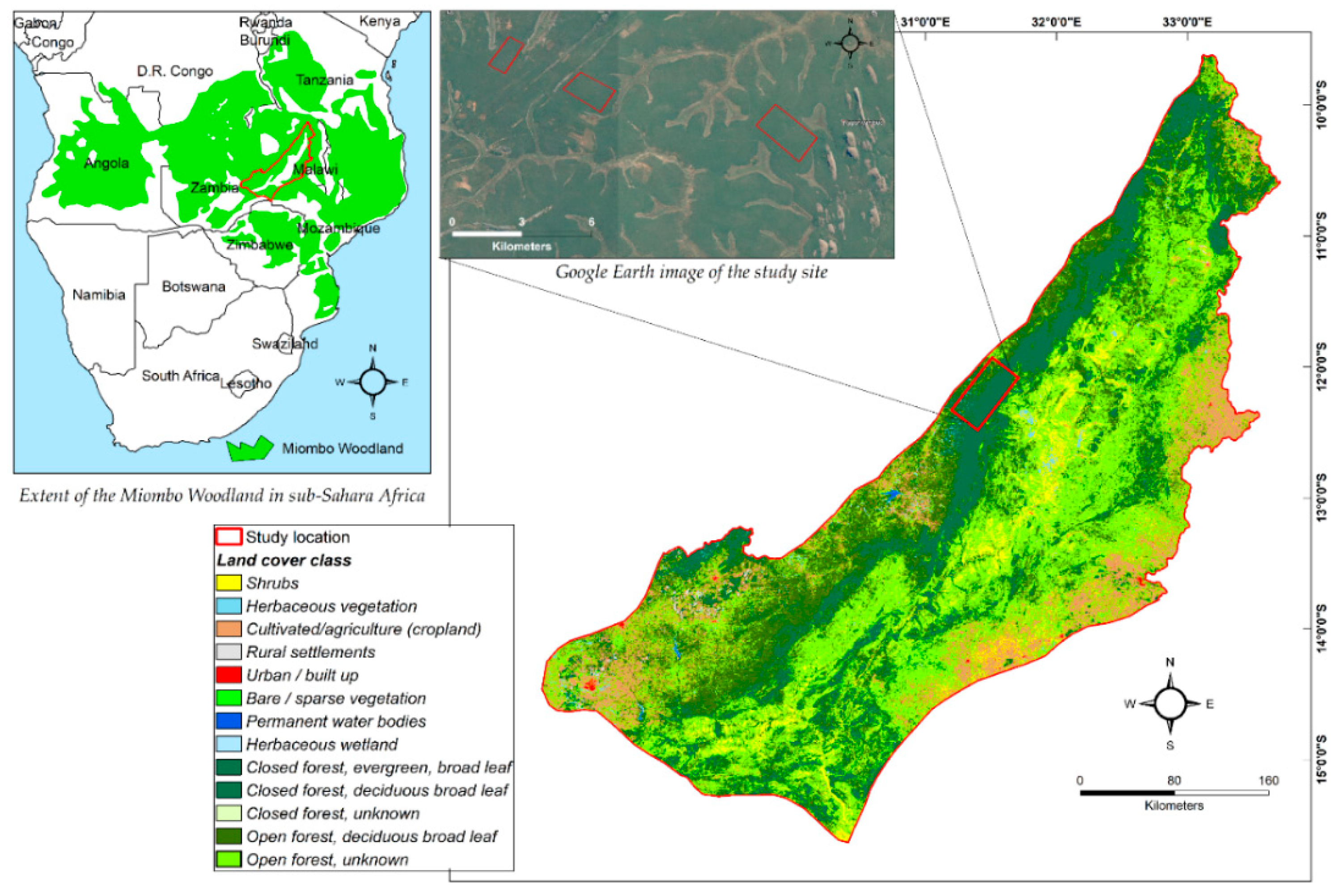
However, the species composition, richness, and heterogeneity (even at local forest level) [2,10,11,12] and the vastness of the Miombo ecosystem in sub-Sahara Africa makes it impossible to employ field observations at a scale capable of capturing an acceptable representation of, for instance, the various plant-water and plant-temperature dynamics of the ecosystem. For instance, field data-based studies like Vinya et al. [13] and Chidumayo [14] only considered a few Miombo species out of the many that exist in the Miombo ecosystem. Furthermore, in addition to financial limitations, field observations normally are spatially and temporally constrained. This has possibly contributed to the paucity of data on the various aspects of forest-climate interactions in the Miombo ecosystem. The application of satellite based remote sensing techniques in assessing forest-climate interaction provides a significant and expanded platform for data collection and monitoring of the dynamic state of forests, especially for vast transboundary woodlands like the Miombo Woodland where ground-based methods are virtually not feasible. This is because satellite remote sensing comes with the advantage of area coverage (spatial resolution), regular revisit time (temporal resolution), acquisition of data in a wide range of the electromagnetic spectrum (spectral resolution), and has a high degree of homogeneity. Furthermore, a large number of satellite sensors, with global coverage, are currently generating enormous amounts of data at various resolutions that form the base for both historical and continued monitoring of forest-climate interactions [15,16,17,18]. This is even more important for Africa with limited capacity to undertake field measurements.
Some studies, including satellite data-based ones, related to plant-water and plant-temperature interaction, have been done in the Savannah woodland, specifically in the Miombo Woodland [13,14,19,20,21,22]. However, the type of satellite data used and the climate variables considered leave room for further investigations using other freely available satellite data products such as the moderate resolution imaging spectroradiometer (MODIS). For instance, most previous studies used air temperature and rainfall to understand the plant water and plant-temperature relationships in the Miombo Woodland. These studies suggested that the Miombo Woodland was water controlled and that temperature could be a critical determinant of plant distribution [13,14,19,20,21,22]. The satellite data-based studies typically used air temperature and normalized difference vegetation index (NDVI) [23] (i.e., Chidumayo [14]), the leaf area index (LAI), transpiration and vegetation optical depth (VOD) (i.e., Tian et al. [19]) to understand the relationships. Chidumayo [14] analyzed the relationship between rainfall, minimum, and maximum air temperature with the NDVI. Chidumayo [14] observed that the combined minimum and maximum temperature accounted for the largest variation (R2 0.96) in NDVI values followed by rainfall (R2 = 0.35). Further, Chidumayo [14] observed a negative relationship between NDVI and maximum temperature. Tian et al. [19] studied seasonal variations in ecosystem-scale plant water storage and their relationship with leaf phenology. They found that in the Miombo Woodland transpiration co-varied with LAI seasonal variations. They further observed that plant water storage played a critical role in “buffering seasonal dynamics of water supply and demand, as well as sustaining fresh leaves formed before the rain”.
However, climate variables such as land surface temperature (LST), which is the radiative skin temperature of a surface derived from remotely sensed thermal radiation, is increasingly becoming more useful in hydrological modelling, vegetation monitoring, global circulation models (GCM), and many more applications [24,25,26,27,28,29,30,31]. The surface temperature is regarded as a direct representation of the canopy thermal status due to its interaction with radiation (long wave and short wave) and other biotic and abiotic processes [30]. The land surface temperature (LST) is considered as a significant variable in controlling several environmental factors including the hydrology, carbon cycle, and land surface energy budget [31]. In the case of the Miombo Woodland, Mildrexler et al. [32] showed that during the dry season, with reduced canopy cover, the LST is higher than air temperature in African Savannah woodland. Furthermore, during the period of high moisture (i.e., rainy season) and high canopy cover maximum LST is almost 1:1 ratio with the maximum air temperature. The surface in the case of the Miombo Woodland would largely be the forest canopy. The discrepancy between LST and air temperature in the dry season could possibly render different results from those observed with the use of air temperature. This makes it necessary to understand the LST (as proxy for canopy temperature) interaction with canopy cover proxies such as the LAI and NDVI. Based on increased application of LST in vegetation monitoring and climate and hydrological modelling the use of LST to understand the canopy cover and canopy temperature relationship in the Miombo woodland could be a significant addition to the body of knowledge on the Miombo ecosystem.
In the context of plant water assessment using satellite data, Mobasheri and Fatemi [33] showed that there exists strong correlation between equivalent water thickness (ETW) (defined as the weight of water per unit area of leaf) and the near infrared (NIR) and shortwave infrared (SWIR) wavelengths in the electromagnetic spectrum. Additionally, they showed that band combinations such as ratio and normalized difference had higher regressions with leaf water content. Some satellite data-based indices such as the normalized difference infrared index (NDII) [34], a normalized band ratio, have shown capacity as proxy for both the vegetation water content and root-zone storage and is, therefore, being used in hydrological modelling [35,36,37,38,39]. When plant water balance is considered, rainfall can generally be assumed as the gross water received in a forest [7,40]. The vegetation water content and root-zone storage (i.e., as proxied by NDII) can be considered more representative of the net water available for use by plants. What is also important is that the NDII can be derived from freely available optical satellite data from sensors such as the MODIS. Therefore, instead of the use of the VOD as proxy for vegetation water [19] or rainfall to indicate water availability [14] this study used the NDII as proxy for canopy water content.
When it comes to observing canopy display and vegetation density the LAI (i.e., the one-sided green leaf area per unit ground surface area in broadleaf canopies [41]) and the NDVI [23] (i.e., measure of density of vegetation) have been used to assess canopy cover in dry forests of Africa and the Miombo Woodland [14,19,42]. For instance, Fuller et al. [42] used the radiative transfer model to demonstrate the NDVI as a good predictor of canopy cover in the Miombo Woodland in Zambia. In this study MODIS based LAI and the NDVI were utilized as proxies for canopy cover.
The premise for the use of the MODIS data is that it is readily available for free, has a near-global spatial coverage (250 m–1 km) suitable for assessing vegetation dynamics in a vast forest like the Miombo Woodland, has a comparatively better temporal scale (1–2 times/day), and can easily be processed with most available imagery computing applications. Other than the availability of raw data MODIS also has several ready to use highly processed products including but not limited to vegetation indices, land surface temperature and evaporation [25,41,43,44,45,46,47,48,49]. These attributes make MODIS data suitable for application at local, catchment and regional scales in a cheaper and timely manner especially in the African context with limited capacity to deploy field-based assessments.
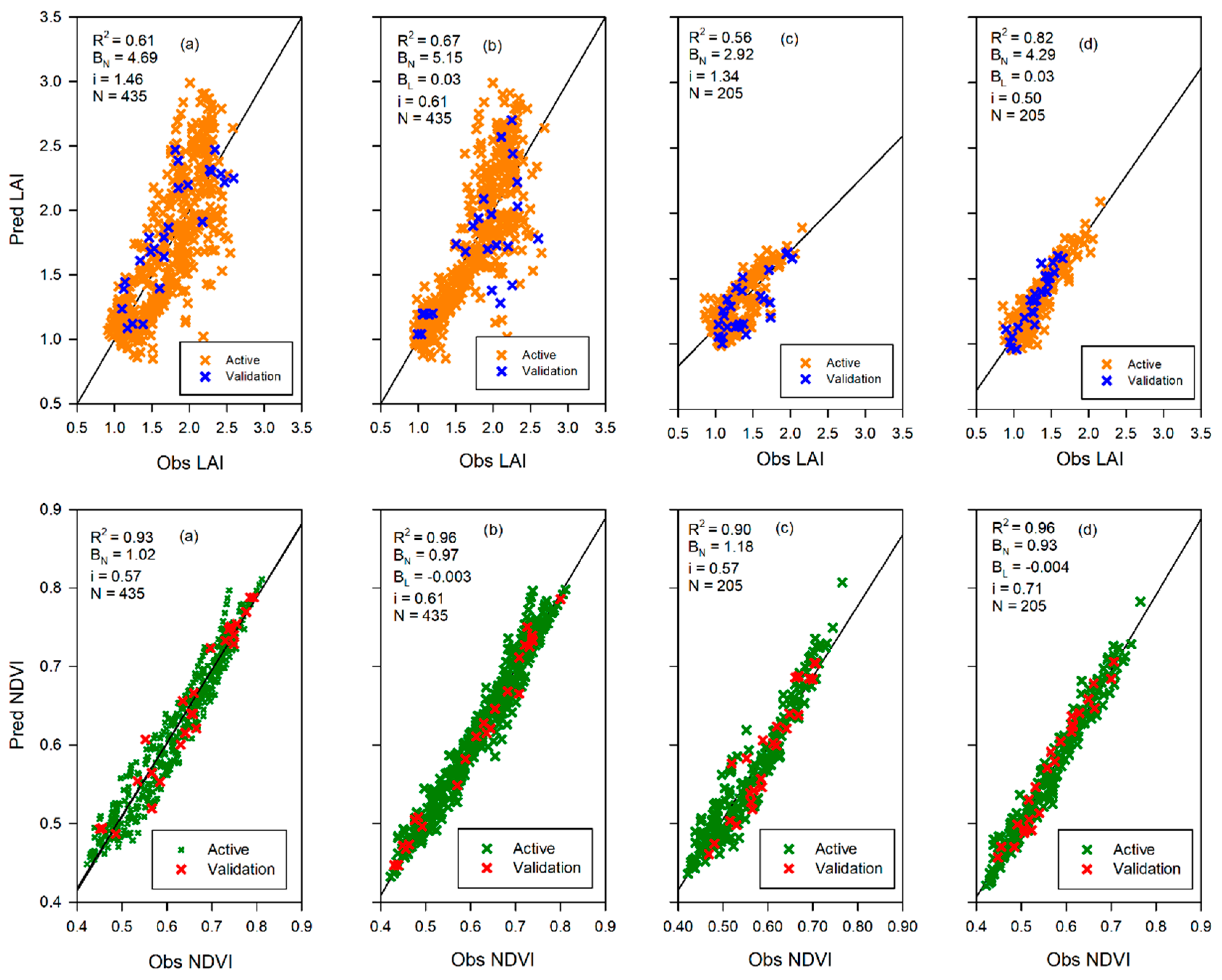
To better understand the interaction of canopy cover with canopy water content and canopy temperature this study used several statistical approaches. Key among the statistical analyses was the correlated component regression linear model (CCR.LM) [50]. The most significant attributes for selecting the CCR.LM were the capacity to account for multicollinearity in predictor variables and to eliminate less important predictor variables, using the step-down variable reduction approach, based on importance in affecting the response variable. By using the CCR.LM we sought to evaluate which of the two variables, i.e., canopy water content (proxied by NDII) and canopy temperature (proxied by LST), accounted for the most variations in the canopy cover at different time scales and seasons. This was important for comparison with the previous studies that used rainfall and air temperature to analyze the interactions with canopy cover.
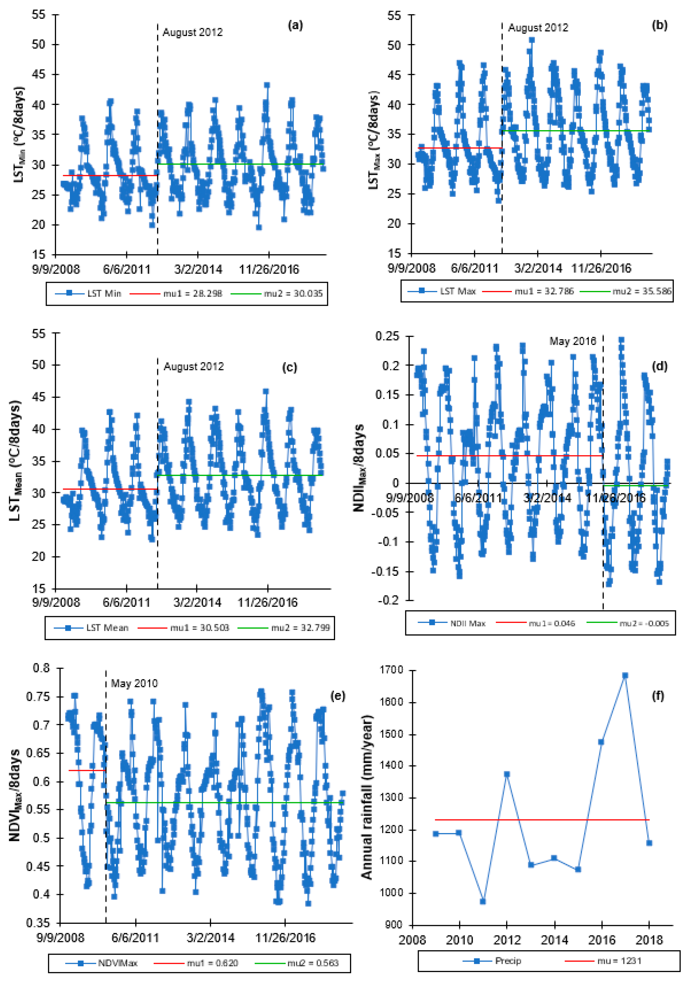
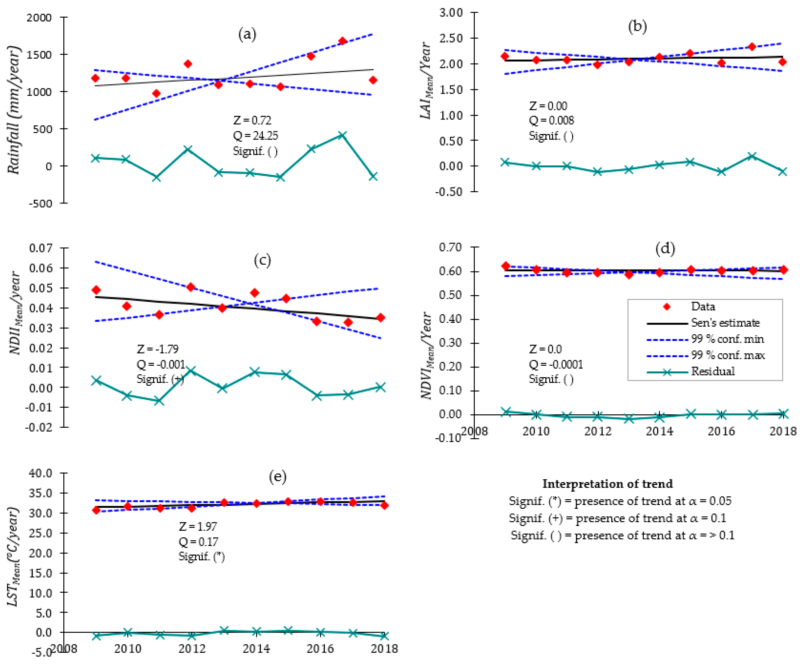
This paper, therefore, describes the results of the assessment of the variations in canopy cover (proxied by the LAI and the NDVI) and its relationship with canopy water content (proxied by the NDII) and temperature (proxied by the LST) in the Miombo Woodland using MODIS satellite based-data. The objectives of this study were to: (i) analyze the seasonal and inter-annual patterns in canopy cover, canopy water content, and canopy temperature; (ii) ascertain the correlation of canopy cover with canopy water content and canopy temperature; (iii) determine the most determinant factor of variations in the canopy cover between canopy water content and canopy temperature in the Miombo Woodland; and (iv) observe if any significant change points and historical trends in the means of the canopy cover, canopy water content, and canopy temperature occurred from 2009–2018. The analysis of change points and historical trends was meant to further understand the relationships between canopy cover, canopy water content, and canopy temperature in the Miombo Woodland. The results of the study could be useful in monitoring the impacts of climate change on the Miombo Woodland phenology.

2. Materials

2.1. Study Site

Miombo Woodland is situated within the southern sub-humid tropical zone of Africa with a mean annual precipitation and mean annual temperature in the range 710–1365 mm/year and 18.0–23.1 °C, respectively. In the Luangwa Basin, in Zambia, where the study was focused (Figure 1), the rainy season is between October and April of a hydrological year. The dry season, May to October, is split into the cool-dry (May to August) and hot-dry (August to October). The rainfall is a result of the movements of the inter-tropical convergence zone (ITCZ) over Zambia between October and April of a hydrological year [2,51,52]. The study was centered on Miombo forest at Nsansala and Mutinondo conservancy areas (Lat: −12.4, Long: 31.2) in the Mpika District, which falls in the central Zambezian Miombo, in the northwestern part of the Luangwa Basin (Figure 1). The location is a conservancy with extremely limited and controlled anthropogenic activities.
The forest is largely in its natural state. The central Zambezian Miombo is the largest of the four Miombo sub-groups the other three being the Angolan Miombo, Eastern Miombo, and the Southern Miombo [53]. According to Frost [2], Zambia has possibly the highest diversity of trees and is said to be the center of endemism for Brachystegia, with 17 species. The Miombo is a heterogeneous forest of the genus Brachystegia with the dominant species in the study location being Brachystegia longifolia, Brachystegia boehmii, Brachystegia speciformis, and Jubenerdia paninculata. Leaf fall and leaf flush occur in the dry season between May and October [2,10,13,52].

2.2. Description of Data Sets

Climate and hydrological data (i.e., modelled precipitation) were retrieved from the National Ocean and Atmospheric Administration (NOAA) Climate Forecast System Reanalysis (CFSR) model, which uses satellite data [54,55] at 19,200 m (1/5-deg) spatial and daily temporal resolution using the Climate Engine. The daily precipitation values were summed into 8-day values to match the temporal resolution of the rest of the data sets.
MODIS surface reflectance (MOD09A1/MYD09A1) [47] data used to compute the NDVI and NDII at 8-day temporal scale and 500 m spatial resolution was obtained using the MODIS global subset tool. MODIS surface reflectance (MOD09A1/MYD09A1) is a 7-band level 3 surface reflectance product with band characteristics as indicated in Table 1. Each product pixel contains the best possible level 2 gridded observation during an 8-day period as selected on the basis of high observation coverage, low view angle, absence of clouds or cloud shadow, and aerosol loading. The MOD09A1/MYD09A1 product has been corrected for the effects of atmospheric gases and aerosols [47].
The NDVI is estimated using the ratio based on the red (R) and near infrared (NIR) bands in Equation (1), while the NDII is estimated using ratios of different values of near infrared reflectance (NIR) and short-wave infrared reflectance (SWIR), as expressed in Equation (2).
NDVI =   ( NIR RED ) ( NIR   +   RED )
NDII =   ( NIR SWIR ) ( NIR + SWIR )
where, in the case of MODIS surface reflectance, Red is B01, NIR is B02, and SWIR is B06 (Table 1).
Satellite data-based LAI (MCD15A2H/MYD15A2H) [41] at an 8-day interval and 500 m spatial resolution were obtained using the MODIS global subset tool. The LAI algorithm consists of a main look-up table (LUT)-based procedure that exploits spectral information content of the MODIS red (648 nm) and NIR (858 nm) surface reflectance and the back-up algorithm that uses empirical relationships between the NDVI and canopy LAI and the fraction of absorbed photosynthetically active radiation (FPAR).The MODIS LAI algorithm accounts for sun-sensor geometry. To augment the observations from the LAI and NDVI the MODIS phenology data the collection 6 MCD12Q2 (C6 MCD12Q2) [56] was used. The C6 MCD12Q2 derives phenometrics from the 2-band enhanced vegetation index (EVI) calculated from MODIS nadir bidirectional reflectance distribution function adjusted surface reflectance time series (NBAR-EVI2). Valid vegetation cycles within the series are identified and records phenometrics for each vegetation cycle [56].
LST (MOD11A2 and MYD11A2) [29] day and night values at 8-day intervals and 1 km spatial resolution were obtained using the MODIS global subset tool. The LST and emissivity daily data are retrieved at 1 km pixels by the generalized split-window algorithm. There are uncertainties associated with satellite-based LST, especially during hot humid periods and for a cold and dry atmosphere [25]. During the rainy season (i.e., hot humid period) LST quality information showed that most pixels had a data quality pass below 80%. Data from pixels with below 100% quality pass was removed and gaps filled by interpolation. However, over 98% of the pixels from which data was retrieved in the dry season (i.e., including the cool-dry season) had 100% quality pass. The LST data was converted from Kelvin to degrees Celsius.
Actual evaporation (Ea) (MOD16A2/MYD16A2) [49] at 8-day interval and 500 m spatial resolution was also obtained using the MODIS global subset tool. The MOD16A2/MYD16A2 uses the Penman–Monteith equation [57,58] and is a sum of night-time and day-time actual evaporation. It is the sum of the evaporation from the wet canopy surface, the transpiration from the dry canopy surface, and the evaporation from the soil surface [49]. In this study, the term evaporation is used instead of evapotranspiration. This is based on the arguments by Miralles et al. [59] and Savenije [60] in which they showed that the term evapotranspiration has limitations and can even be considered as misleading.
All MODIS based data used in this study had quality reports. Based on the quality report all data from pixels with below 100% quality pass, especially during the rainy season, were removed and then the gaps were filled by interpolation. The data sets from the MODIS terra and MODIS aqua sensors (i.e., MOD16A2 and MYD16A2, MCD15A2H and MYD15A2H, MOD11A2 and MYD11A2) were summed up per variable and averaged to come up with Ea, LAI, and LST data sets. Polygons for each of the Miombo Woodland location(s) (Figure 1) were used to extract the required data sets from January 2009 to December 2018. Raw filtered data provided on the global subset tool was used to estimate the 5th and 95th percentiles for the variables. The focus of the study was the dry season and had most pixels with acceptable quality pass of 100%.

3. Methods

3.1. Study Approach

The study evaluated the canopy cover relationship with canopy water content and canopy temperature in the Miombo Woodland using satellite data. To track and evaluate changes in the forest canopy cover the LAI and NDVI were used as proxies for canopy cover [23,41,61,62,63], the NDII as a proxy for canopy water content [34,36,38] and the LST [28,29,64] as a proxy for canopy temperature [1]. The LAI, NDII, and NDVI make use of the NIR region of the electromagnetic spectrum. In addition, since actual evaporation (Ea) and rainfall are closely linked to the LAI, LST, NDII, and NDVI [30,31,32,36,65,66], they were used to augment the observations in the general patterns of the LAI, LST, NDII, and NDVI, but were not included in the statistical analyses as predictor or response variable. Furthermore, the phenology calendar was used to augment the LAI and NDVI observations.
We analyzed a 10-year period (2009–2018) in order to capture long term variations in the data. In the Luangwa Basin, hydrological year is categorized as the period from September to August. The rainy season is between November and April while the dry season is between May and October [51]. Three polygons were used to retrieve the data in a 30 km by 30 km (900 km2) area in the Miombo Woodland at Nsansala and Mutinondo conservancy areas (Figure 1). The conservancy areas were selected due to availability of a dense Miombo Woodland which is protected and is with minimal anthropogenic disturbances. The data for each variable from the three polygons was merged into one data set per variable and analyzed. To avoid mixing variables values from different land cover types (i.e., grassland, bare soil, and other forest types) with Miombo Woodland the assessment was restricted to a dense Miombo Woodland (Figure 1). Hence, the assessment was not done at the entire Miombo ecosystem level in Africa but restricted to this dense Miombo woodland in the Luangwa Basin in Zambia.
The statistical analyses included testing for outliers with the Dixon test and Z-score approach. We tested for homogeneity and monotonic trends with the Pettit test and the Mann–Kendall trends test. Analysis of variation was done with the analysis of variance (ANOVA) approach. Analysis of correlations was done with the Pearson r, while the CCR.LM was used to understand the influence of predictor variables on response variables. The methods are briefly explained in Section 3.2 below.

3.2. Statistical Approaches Used to Analyse the Data

3.2.1. Testing for Outliers with the Dixon Test

We used the Dixon test [67] to assess if the data sets contained outliers at either end points, i.e., highest and lowest values in the data sets. The Dixon test is a process developed to help ascertain if the greatest value or lowest value of a sample, or the two largest values, or if the two smallest ones can be considered as outliers. The test works based on the assumptions that the data corresponds to a sample extracted from a population that follows a normal distribution. The null hypothesis is that there are no outliers in the data. The outlier is said to be significant if the test statistic value is lower than the critical value from the Dixon test table. Further examination of data for outliers was done with the Z-score analysis approach. The Z-score defines the position of a raw score with reference to its distance from the mean when measured in standard deviation units. The Z-score is positive if the value lies above the mean, and negative if below.

3.2.2. Assessing Correlation of Variables with the Pearson R Approach

Pearson’s r [68] is the most commonly used measure of correlation [69]. It is sometimes referred to as the linear correlation coefficient because of its measure of linear association between two variables. Pearson’s r is a dimensionless property obtained by standardizing and dividing the distance from the mean by the sample standard deviation. The significance of r is determined by testing whether r differs from zero. The test statistic is compared to a table of the t distribution with n − 2 degree of freedom. The Pearson r value ranges between −1 and +1, with −1 indicating that the two variables are perfectly negatively linearly related, while +1 indicates that the two variables are perfectly positively related. The closer the Pearson r value to either −1 or +1 the stronger the correlation [69].

3.2.3. Assessing Variations in the Variables with the RM-ANOVA

The repeated measure analysis of variance (RM-ANOVA) [69] is a commonly used typical parametric test that helps ascertain whether samples in more than two groups have the same central value (mean or median) or whether one of the groups has the central value different from others. Reliability of the RM-ANOVA is dependent on the fulfilment of the assumptions that variables are independent and identically distributed, variable residuals are normally distributed (or approximately normally distributed), and the variances of populations are equal. The total variation of all the observations about the overall mean is measured by what is called the total sum of squares.
The null hypothesis is that there are no variations in the population means, while the alternative hypothesis is that there are variations in the population means. To test for the null hypothesis, the F statistic is used. The F statistic is compared with the F distribution with k 1 and N k degrees of freedom. The F statistic is approximately equal to 1 if the null hypothesis is true but will be larger than 1 if there are differences between the population means. Significance of the variations in the population means is ascertained by the p-value, which simply expresses the probability of having the means constant or not constant. If the means are constant or not further apart, the p-value is very large (no significant variations). If the means are wide or further apart (significant variation exists), the p-value is very small (<0.00001) [69].

3.2.4. Correlated Component Regression Linear Model (CCR.LM)

The correlated component regression (CCR), developed by Magidson [50], is an ensemble dimension reduction regression technique which utilizes the K correlated components to predict the dependent variable. It is equivalent to the corresponding Naïve Bayes solution for K = 1 and equivalent to traditional regression for K = P with P predictors. The application of the Naïve Bayes rule deals with the effects of multicollinearity among predictor variables. In the CCR-linear algorithm, the outcome variable Y is predicted by K correlated components, each a linear combination of the predictors X1, X2,……, XP. The CCR-linear algorithm is a generalization of the CCR-logistic and is generally performed in three steps. Step 1: the first component S1 captures the effects of prime predictors that have direct effects on the outcome. It is an average (ensemble) of all 1-predictor effects: Step 2: the second component S2 is correlated with S1 and captures the effects of suppressor variables (proxy predictors) that improve prediction by removing extraneous variation from S1. Step 3 estimates the 2-component model using S1 and S2 as predictors. The predictions (coefficients of estimates) for Y in the K-component CCR model are obtained from the ordinary least square regression of Y on S 1 ,……,   S k . The regression coefficient for predicting a variable is simply the weighted sum of loadings, where the weights are the regression coefficients for the components in the K-component model. The step-down variable reduction step for a given K-component model eliminates the least important predictor variable, where importance is quantified as the absolute value of the variable’s standardized coefficient. If a predictor variable is found to have the least absolute value of the standardized coefficient, the predictor is excluded and the steps of the CCR estimation algorithm repeated on the reduced set of predictors. The regression correlation coefficient of determination (R2) and the normalized mean square error (NMSE) [50,70] are used to assess the performance of the CCR.LM in predicting the response variable(s) with a given combination of predictor variables.

3.2.5. Testing for Homogeneity with Pettit Test

To observe if there were any significant abrupt changes (i.e., due to changes in climate, change in land cover type and other factors) in the means of the variables, we used the Pettit [71] homogeneity test. The Pettit homogeneity test approach is a common non-parametric application in change point detection studies involving hydrological or climate series which are known to be non-normal data [69,72]. The test statistic counts the number of times a member of the first sample exceeds a member of the second sample. The null hypothesis is that the data are homogenous, i.e., absence of a change point. The test statistic is said to indicate a significant change point when the associated probability ≤ 0.05. When a significant change point is found, the time series data are divided into two parts at the location of the change point. The Pettit test is then conducted on the time series from which the change was detected to see if any further changes occurred [69].

3.2.6. The Mann–Kendal Trends Test and the Sens’ Method

The Mann–Kendall test [67,73,74] used in this study was chosen premised on the advantages it possesses over other tests, such as being a non-parametric test that does not need the data to be normally distributed and its low sensitivity to abrupt changes due to inhomogeneity in time series data. In general terms, the Mann–Kendall test seeks to establish whether monotonic changes are present in a given set of random values. The test statistic represents the number of positive differences minus the number of negative differences for all the differences between adjacent points in the time series. Positive values indicate an upward trend while negative values indicate a downward trend. The test statistic is used to test the null hypothesis and is a measure of the strength of the trend. The null hypothesis is that there is no trend in the series, while the alternative hypothesis is that there is a trend in the series. If the computed p-value is greater than the chosen significance level (i.e., alpha level = 0.05 used in this study), the null hypothesis is accepted while the alternative hypothesis is accepted if p-value is less than the significance level.
The Sens’ method [75] is a non-parametric approach used to estimate magnitude of trends in data time series. The Sens’ method can be used in cases where the trend can be assumed to be linear. It estimates the slope of “n” pairs of data. The Sens’ estimator of slope is the median value of these N values of the slope estimate. To obtain the slope estimator the N values, the slope estimates were ranked from smallest to largest. Lastly, a two tailed test at 100 (1 − α) % confidence interval was used to test the slope estimate with a non-parametric technique based on the normal distribution [76].

4. Results

4.1. Assessment of Outliers with the Dixon Test and Z-Score Approach

Assessment for outliers in the data was done with the Dixon test. The data was first categorized into sample population of n ≤ 100 based on the seasons, i.e., rainy season and dry season (categorized into cool-dry and hot-dry). The data was then tested for outliers on each category. Table S1 gives some of the results for the Dixon test. Across seasons, no statistically significant (p-value > 0.05) outliers were detected. However, further analysis with the Z-score values showed that some variables had some outliers. These were removed and the gaps filled by interpolation. For instance, Z-score values showed some LAIMax values to be outliers. The LAIMax outliers were lowest values of 1.1 observed on the 7th and 20th of July 2009, 20th and 13th of August 2011, and also on the 13th and 19th July 2012. These observations can possibly be attributed to underestimation by the LAI algorithm as the observations were for shorter periods between two points with higher values on both ends (before and after). Furthermore, these outliers in LAIMax were not linked to any changes in the LST, NDII, or NDVI on the same dates or period. For the LST, some outliers were mostly flagged in the rainy season, which is possibly due to the associated challenges in assessing LST in hot-humid environments. The rainy season LST “outliers” could also indicate drought periods during the rainy season though this was discounted based on the counterchecking with rainfall, LAI, NDII, and NDVI values for the same dates/period(s). In general, the test for outliers showed that there were no extreme events in the variables examined for the period 2009–2018 in the study area.

4.2. Pattern Observed in Phenology, Canopy Cover, Water Content and Temperature

Based on the phenological observations by collection 6 MCD12Q2 data, shown in Figure 2, it was noticed that senescence (i.e., process of leaf aging) generally occurred between January and March in the rainy season. The green down (i.e., reduction in green color in leaves due to reduction in chlorophyll) was normally reached between March and May while the dormancy state (i.e., state of temporary metabolic inactivity or minimal activity) was mostly attained between May and July.
The green up (i.e., increase in green color in leaves due to increase in chlorophyll and metabolic activity) was noted to normally start around October in the dry season, reaching its peak between December and January. Figure 3 and Figure 4 illustrates the temporal patterns in variables. In the case of Figure 3 the period 2017 to 2019 was used to illustrate the temporal patterns in the variables. There seemed to be synchronism between the phenology calendar and the changes in canopy cover values (i.e., LAI and NDVI) and the canopy water content (i.e., NDII). Canopy cover peak was observed during the rainy season between January and February (Figure 3a and Figure 4), the same period when phenological maturity was attained (Figure 2). Minimum canopy cover was observed during the dry season between August and September during the dormancy state (Figure 2, Figure 3a, and Figure 4). During this period the canopy cover (proxied by LAI and NDVI) showed synchronism with the canopy water content and the actual evaporation (Figure 3). A sharp decline in the LAI, NDVI, and Ea were observed at the end of the rainy season in April.
The start in decline in variables in Figure 3 coincided with the green-down phenological phase in Figure 2. There appeared to be a time lag of about one to two months between the LAI and the NDVI as to the start in the rise in canopy cover (Figure 3a) in the dry season. Generally, the LAI begun to rise in mid-August while NDVI started at the beginning of October.
A start in steady decline in canopy cover (i.e., both LAI and NDVI) was observed in May, one month after the end of April’s rainy season (Figure 3a and Figure 4), which happens to be the same period when vegetation enters dormancy (Figure 2). However, there was a difference when canopy cover increased with maximum LAI values, indicating mid-August, while NDVI seemed to show at the end of October (Figure 4). Peak canopy water content (i.e., NDII) was observed in the rainy season between December and February, while the lowest values were observed in the dry season in September (Figure 4). The peak and lowest canopy water content corresponded with the peak and dormancy stages in the phenology. The canopy water content declined in May following the end of April’s rainy season. However, it was surprising that canopy water content (i.e., NDII) like canopy cover (i.e., NDVI) increased in the hot-dry season in October before the commencement of the summer rains (Figure 3a and Figure 4). However, like with canopy cover, canopy water content started to increase in October before the commencement of the summer rains (Figure 3a and Figure 4).
The periods for the lowest and highest canopy temperature (i.e., LST) values corresponded with the dormancy and green-up phenological stages (Figure 2 and Figure 3a). One important observation was that there seemed to be synchronism between the Ea and the canopy cover (i.e., LAI and NDVI) and the canopy water content (i.e., NDII) across seasons (Figure 3 and Figure 4).

4.3. Analysis of the Observed Patterns with the RM-ANOVA Test

The RM-ANOVA results for the comparison between the rainy and dry season values of variables and the inter-annual comparison of the dry season values of variables are shown in Table 2 and Table S2. The LAI, LST, NDII, and NDVI values for the rainy season significantly (p-value < 0.05) differed with the dry season values. Other than the LST high values of variables were observed in the rainy season, while the lowest values were observed in the dry season. The opposite was true for the LST with the high and lowest values both occurring in the dry season. The differences in terms of the means were 2.32, 2.48 °C, 0.15m and 0.13 for LAI, LST, NDII, and NDVI, respectively. The dry season values of LAI, NDII, and NDVI significantly (p-value < 0.05) differed across the years (2009–2018), while the LST values did not show significant (p-value = 0.805) differences. However, further analysis involving the all pairwise multiple comparison with the Holm–Sidak method showed that values of variables between some years were not significantly different (Table S3 in the supplementary data).

4.4. Pearsonr Correlation Analysis of the Relationship of Variables

Minimum, maximum, and mean values of variables were analyzed for correlation. Mean values were used to demonstrate the relationships among variables across seasons. Figure 5 shows the annual (January–December) correlation plots using mean values of variables. Table 3 gives the results of the correlation statistics of variables at annual scale. Detailed correlation statistics for the rainy and dry seasons are shown in the supplementary data (Tables S4–S7). In Figure 3 and Figure 5, there seemed to be hysteresis behavior between LAIMean and NDIIMean, as well as between LAIMean and LSTMean, indicating that changes in canopy cover (i.e., LAIMean) lagged behind changes in canopy water content (i.e., NDIIMean), as well as changes in canopy temperature (i.e., LSTMean). The changes in the canopy cover was not only affected by the canopy water (i.e., NDIIMean) and temperature (i.e., LSTMean) in a given day but by cumulative canopy water and temperature conditions. Generally, canopy cover (i.e., NDVIMean) showed synchronism with canopy water content (i.e., NDIIMean) throughout the year. Canopy cover (in the case of LAIMean) only showed strong correlation with canopy temperature during the hot-dry season. Statistically, at the annual scale, the canopy water content (i.e., NDIIMean) relationship with canopy cover (i.e., LAIMean and NDVIMean) was strongly positive with r = 0.78, 0.97 with p-value < 0.0001, respectively (Figure 5 and Table 3).
At rainy and dry season scales, the canopy water content (i.e., NDIIMean) versus canopy cover (i.e., LAIMean and NDVIMean) correlation was strongly positive except for the NDII-LAI relationship, which showed a low coefficient of correlation (i.e., r = 0.29 and p-value < 0.008) for the rainy season (Tables S4–S7 in the supplementary data). However, during the hot-dry season, strong NDII-LAI correlation was observed with r = 0.70 and p-value < 0.0001 (Table S7). Generally, NDII-NDVI correlations were stronger (i.e., r > 0.75) across all seasonal scales (Tables S4–S7 in the supplementary data). Table 3 and Tables S4–S7 in the supplementary data gives statistics of the Pearson r correlation analysis of the canopy temperature (i.e., LST) correlation with canopy cover (i.e., LAI and NDVI). At the annual scale, the canopy cover (i.e., LAIMean as a proxy) negatively covaried with canopy temperature with r = −0.11 and p-value < 0.83. When canopy cover was proxied by NDVI a negative covariation with canopy temperature of r = −0.41 and p-value < 0.0001 was observed. During the rainy season, the LST-NDVI relationship showed a correlation coefficient of r = −0.44; and p-value < 0.0001, while LST-LAI correlation had r = −0.52; and p-value < 0.001.During the dry season (May–October), the LAI-LST correlation was positive but weak and statistically insignificant with r = 0.04 and p-value = 0.56. The NDVI-LST correlation was negative but relatively stronger with r = −0.68 and p-value < 0.0001. During the cool-dry season (May–July) the NDVI-LST correlation was positive but relatively weak (r = 0.26, p-value < 0.0046), and was the same as the LAI-LST relationship (r = 0.26, p-value < 0.0044) (Tables S4–S7 in the supplementary). However, the hot-dry season (August–October) showed stronger positive LAI-LST correlation (r = 0.62, p-value < 0.0001), while the NDVI-LST relationship was negative (r = −0.25, p-value = 0.0097) (Tables S4–S7 in the supplementary). Generally, at the annual scale, LSTMin values showed relatively stronger correlation with LAIMin and NDVIMin compared to the LSTMax and LSTMean values (Table 3).

4.5. Regression of Canopy Cover Relationship with Canopy Water Content and Canopy Temperature Using the CCR.LM

Figure 6, Table 4 and Table 5, and Tables S8–S10 show results of the CCR.LM. First, regression was done with mean values of individual predictor variables and later inputted simultaneously. This was done to benchmark the relationship of LST and NDII with LAI and NDVI exclusive of the other predictor variable. The second part of the regression was the relationship of the canopy cover (i.e., LAI and NDVI) with both canopy water content (i.e., NDII) and canopy temperature (i.e., LST) used simultaneously as input variables. This enabled the assessment of the combined influence of the variables on the variations in the canopy cover. Figure 6 and Table 4 and Table 5 show the CCR.LM results during the annual and dry season scales. Tables S8–S10 (in the supplementary data) give the CCR.LM unstandardized coefficients of estimates and cross validated goodness of fit statistics for each regression for the rainy, cool-dry and hot-dry seasons. There was no collinearity between LST and NDII.
The NMSE and the coefficient of determination (R2) were used to assess the estimate of the overall deviations between predicted and “observed” values, thus ascertaining the performance of the model. The unstandardized coefficients ( ß ^ ) were used to analyze which of the input variables (i.e., LST or NDII), at each run, had a significant effect on each response variable (i.e., LAI and NDVI) at different time scales, i.e., annual and dry season
At the annual scale, the NDII as a single variable accounted for 61% (R2 = 0.61) of the variations in LAI and 93% (R2 = 0.93) in NDVI. LST as a single variable accounted for 13% in LAI variations and 17% in NDVI variations (Table 4). A combination of the LST with NDII accounted for about 67% (R2 = 0.67) of the variations in LAI and 96% (R2 = 0.96) in NDVI improvements of 9.83% and 3.22%, respectively. Further analysis of the coefficients of estimates showed that the NDII had the most influence on variations in canopy cover with coefficient estimates of ß ^ = 0.03, −0.003 and ß ^ = 5.15, 0.97 for LST and NDII on LAI and NDVI, respectively (Figure 6 and Table 4). When analyzed for the rainy season scale (November–April), the most determinant factor of variations in the canopy cover (i.e., LAI and NDVI) were by single variable interactions. For instance, LST as a single variable accounted for 21% of variations in the LAI while interaction between LST and NDII only accounted for 24%. Further, as single variables, the LST and NDII accounted for 50% and 91% of variations in the NDVI, respectively. LST and NDII interaction also accounted for 91% variations in NDVI, the same as the NDII as a single variable (Table S8 in the supplementary data). For the dry season, the NDII as a single variable accounted for 56% variations in LAI and 90% in NDVI. As a single variable, LST accounted for 21% (R2 = 0.21) variations in LAI and 56% (R2 = 0.56) of the variations in NDVI (Figure 6 and Table 5).
During the dry season the combination of LST and NDII as predictor variables accounted for 82% (R2 = 0.82) of the variations in LAI and 96% (R2 = 0.96) in the NDVI (Figure 6 and Table 5). Consequently, adding LST to the regression improved the outcomes by 46.43% and 6.67% in the case of LAI and NDVI, respectively (Table 5). During the annual time scale, the NDII had the most influence on the variations in the canopy cover, as indicated by the coefficients of estimates ß ^ = 0.03, −0.004 and ß ^ = 4.29, 0.93 for LST and NDII on LAI and NDVI, respectively (Figure 6 and Table 5). The interpretation of the coefficients (i.e., for the dry season), with LAI as a proxy for the canopy cover, is that the amount of change (i.e., ß ^ = 4.29) in the canopy cover (i.e., LAI) due to a 1-unit change of canopy water content (i.e., NDII) was higher than the change (i.e., ß ^ = 0.03) in the canopy cover (i.e., LAI) due to a 1-unit change in canopy temperature (i.e., LST) (Table 5 and Tables S8–S10). For every one-unit increment in LST during the hot-dry season, the NDVI was reduced by about 0.01, while for every increase in one-unit of NDII, the NDVI increased by about 1.1 (Table S10 in the supplementary data). The model outputs and overall interpretation for the cool- and hot-dry season analyses (Tables S8–S10) were different than the annual scale results. For the hot-dry season (August–October), the LST, as a single variable, accounted for most variations (35%) in the LAI, while the NDII accounted for most variations (47%) in the NDVI. Furthermore, combination of the LST and NDII as predictors improved accounting for variations in LAI from about 35% (with either LST or NDII) to 68% (with LST and NDII combined) and NDVI from 48% (with NDII only) to 79% (with LST and NDII combined). During the cool-dry season (May–July), LST, as a single variable, had insignificant influence on variations in both LAI and NDVI. On the other hand, the NDII as a single variable accounted for 87% variations in the LAI and 94% in the variations in the NDVI. Thus, a combination of LST and NDII in the cool-dry season did not improve accounting for variations in the LAI and NDVI (Table S9).
Overall, NDII seemed to account for the most variations in both the LAI and NDVI across seasons. However, during the dry season, the LST seemed to account for the most variations in the LAI. Further, despite LSTMin showing relatively stronger correlations with LAIMin and NDVIMin, there were no significant differences observed between the use of LSTMean, LSTMin, and LSTMax in the model.
Generally, for the annual (January–December), dry season (May–October), and cool-dry season (May–July) scales, adding LST to NDII improved accounting for variations in the canopy cover (i.e., LAI and NDVI as proxies) but at varying magnitudes with the most significant contribution noted in the dry season (Table 5 and Table S10 in the supplementary data). Based on the CCR.ML results (Figure 6, Table 4 and Table 5, and Tables S8–S10), changes in canopy water content accounted for the largest variations in canopy cover across seasons.

4.6. Assessment of Abrupt Change in Variables with the Pettit Test

Table 6 and Figure 7 shows results of the Pettit test at the annual scale (January–December), while Table S11a in the supplementary data provides the dry season Pettit test results. For the annual scale (January–December), the Pettit test on the 8-day values of variables indicated only three variables—LST (minimum, maximum, and mean), NDIIMax, and NDVIMax—to have had abrupt change in mean values between the period 2009 and 2018. Daily rainfall values also showed significant downward abrupt changes in 2012 and 2014, and an upward change was observed in 2016. The mean annual and monthly rainfall values, as well as the rest of the variables—i.e., LAIMin, LAIMax, LAIMean, NDVIMin, NDVIMean, NDIIMin, and NDIIMean—did not show any significant abrupt changes in the time space 2009–2018 (Table 6 and Table S11a). The LSTMin, LSTMax, and LSTMean values seemed to have had a significant (p-value < 0.05) abrupt upward change. The NDIIMax and NDVIMax seemed to have had a significant (p-value < 0.05) abrupt downward change in the mean values. At the 99% confidence level, the LSTMin mean value changed from about 28.30 °C between 2009 and 2012 to 30.04 °C between 2012 and 2018. For the same time steps, the LSTMax and LSTMean seemed to have changed from about 32.79 to 35.59 °C and from about 30.50 to 32.80 °C, respectively. The NDIIMax mean changed from 0.05 between 2009 and 2016 to 0.01 between 2016 and 2018. Except for the daily rainfall data none of the other variables showed further change points after the initial change points.
For the dry season scale, the Pettit test showed one-time abrupt change with upward change in LAIMean in September, 2013 from LAIMean value of 1.25 to 1.37, while the NDIIMax and NDVIMax changed downwards in July from −0.03 to −0.07 and 0.52 to 0.49, respectively. There was no change in LST.

4.7. Assessment of Trends in Values of Variables with Mann–Kendall Trends Test

To observe if trends existed in the variables, we performed the Mann–Kendall trends test on all variables. Table 7 and Table S11b shows the results of the Mann–Kendall test for the tested variables. From 2009 to 2018, the Mann–Kendall test revealed existence of significant (p-value < 0.05) trends in some variables with the LSTMin, LSTMax, and LSTMean, indicating an upward trend, while the NDIIMax and NDVIMax revealed significant downward trends with p-values of 0.0187 and 0.0022, respectively. At the alpha level = 0.05, there were significant trends in daily rainfall values (Table 7) but no significant trend in the mean monthly and annual values was observed. However, the negative sign in the S-statistic and the Kendall’s Tau for the mean monthly and annual rainfall data indicated a general downward movement. The direction of the trend is revealed by the S-statistic and the Kendall’s Tau with a positive value indicating an upward trend, and a negative value indicating a downward trend (Table 3).
Annual averages of rainfall, LAI, LST, NDII, and NDVI were analyzed with the Mann–Kendall and Sens’ slope estimate. This was done to find out the possible change in the variables per unit of time (i.e., per year) and if these changes showed any relationship(s). Figure 8 shows the results of the analyses of the annual average data of variables. The Q is the true slope of linear trend and the Z is the test statistic. It was observed that during the period 2009–2018, rainfall generally increased at a rate of 24.25 mm/year, which was significant at alpha level > 0.1. The LAI increased at the rate of 0.008/year at alpha level > 0.1. At alpha level 0.1, the NDII reduced at an annual rate of 0.001/year, while the NDVI reduced at −0.0001/year at alpha level > 0.1.
The most significant rate of change was with the LST, which increased at 0.17 °C/year at alpha level 0.05. In essence, at the alpha level of 0.05, only the LST showed a significant annual rate of change. In general, mean LSTMean and LAIMean increased while NDIIMean and NDVIMean reduced despite the insignificant (at alpha > 0.1) increase in rainfall.

5. Discussion

5.1. Variations in Canopy Cover, Canopy Water Content and Canopy Temperature

Water and temperature have already been advanced as key variables in the Miombo Woodland’s canopy display [2,13,14,19,77]. However, the studies that used remote sensing data such as Chidumayo [14] and Tian et al. [19] used air temperature, LAI, NDVI, rainfall, and the VOD to understand these relationships. In this study, satellite-based LST and NDII were used as proxies for canopy temperature and canopy water content, respectively. Like in other assessments (i.e., Chidumayo [14] and Tian et al. [19]), this study used the LAI and NDVI as proxies for the canopy cover. The observations made in this study in terms of the variations in the canopy cover across seasons were similar to those previously noted by Chidumayo [14] and Tian et al. [19]. The observed variations in canopy cover during the dry season could be attributed to climatic factors such as rainfall. According to Fuller [77] and Frost [2], depending on the amount of rainfall received in the preceding season, some Miombo species may shed leaves early at the commencement of the dry season, especially in the case of low rainfall, or they may keep leaves late into the dry season in the case of high rainfall. These observations are possibly affirmed by the phenology calendar (Figure 2), which shows differences in occurrence of phenological stages across the years. Further, ANOVA analyses in this study found statistically significant inter-annual variations in canopy water content (i.e., NDII) and canopy cover (i.e., LAI and NDVI). In this study, it was observed that canopy cover is highly correlated and in sync with canopy water content. These observations coupled with those by Fuller [77] and Frost [2] demonstrate water as a significant canopy display controlling factor. However, based on the observations in Figure 3 and Figure 4, significant canopy cover, as proxied by LAI and NDVI, decreased immediately following the end of the rainy season. A plausible explanation for the observed sharp decrease in LAI and NDVI in May could be that the remote sensing LAI and NDVI calculations are based on the 500 m by 500 m spatial resolution [41], which potentially includes under canopy grass and shrubs. Under canopy grass in the Miombo Woodland easily dry out at the end of the rainy season when soil moisture reduces [2]. Therefore, the observed sharp decrease in LAI and NDVI in May could be due to reduced canopy closure, wilting and drying of canopy undergrowth, grass, and shrubs [32], as rainfall would have stopped, and soil moisture reduced in the upper layers. Thus, little moisture could sustain grass and shrub turgidity and greenness.
In this study, there seemed to be a minimal discrepancy of about one to two months between when LAI and NDVI values rose in the dry season, with the LAI values appearing to rise in August during the dormant stage while the NDVI rose between the end of September and the beginning of October at the start of the green-up stage (Figure 2, Figure 3 and Figure 4). One plausible explanation for this observation could be that, in some Miombo species, new leaf color transitions during the dry season. Leaf flush in some Miombo species is followed with leaf color transitions from red to yellow to green and occurs at different times for different species with most species undergoing this process between August and October [13,78,79]. The NDVI is sensitive to green vegetation, thus the color transitions may affect the values and possibly results in the observed delay. The start in rise in NDVI values in September/October may suggest that this is when the leaf flush or growth of vegetation component occurs, which is contrary to the field observations [2,13,14]. The start in the rise in mean LAI values in August is likely to be more representative of the occurrence of leaf flush than that of the NDVI in September/October. However, the start in rise in NDVI values in the dry season corresponds with the collection 6 MCD12Q2 start in green-up (Figure 2, Figure 3 and Figure 4). This could suggest LAI as a better proxy for canopy cover during the dry season than the NDVI.
The observed high LST values (Figure 3) in the dry season can be attributed to reduction in canopy cover (i.e., LAI) and vegetation water content (i.e., NDII) (Figure 3 and Figure 4). This is because the increase in LST values in July when LAI values were low could indicate a reduced canopy closure, which exposes the forest floor (normally covered with dry leaves and exposed soil) to direct interaction with radiation resulting in increased surface temperature [30]. Furthermore, the NDII exhibited zero values in June (Figure 3 and Figure 4), which proved that plant water stress is normally attained around this period. LST is used as an indicator for plant water stress and drought [24,80,81]. Therefore, the rise in LST in July could be an indication of plant water stress due to limited water conditions. According to Baldocchi et al. [82] and Mildrexler et al. [32], in the dry season, stomata shut in the savannah trees and the sensible heat fluxes significantly increase. This observation is contrasted by the decline in LST values in October when canopy water content (i.e., NDII) rose (Figure 3 and Figure 4). Most importantly, by October, the canopy cover (i.e., LAI) and actual evaporation increased (Figure 3 and Figure 4), implying that there was an increase in energy demand (i.e., increase in latent heat fluxes) for evaporation, which resulted in a decline of canopy temperature (i.e., LST) [31].

5.2. Canopy Cover Relationship with Canopy Water Content and Canopy Temperature

Contrary to observations with air temperature by Chidumayo [14], this study found that LST, at annual scale, accounted for less variation (i.e., 13% and 17% in the LAI and NDVI, respectively) compared to the canopy water content (61% and 93% in the LAI and NDVI, respectively). For instance, at the Mpika Miombo Woodland site, Chidumayo [14] found that rainfall, as a single variable, accounted for 35% of the variations in NDVI while a combination of minimum and maximum air temperature accounted for 94% of the variations. However, this study revealed that canopy water content (i.e., NDII) and not canopy temperature, as a single variable, accounted for the largest (i.e., 93%) of variations in NDVI, annually. However, the combination of the canopy water content (i.e., NDII) and canopy temperature (i.e., LST) accounted for the largest variation in canopy cover proxies (i.e., 67% in LAI and 96% in NDVI) (Table 4 and Table 5). For the dry season, LST as a single variable accounted for 21% and 56% variations in LAI and NDVI, compared to NDII at 56% and 90% for LAI and NDVI, respectively. This observation highlights the significance of surface temperature in observing phenological responses during the seasonal drought in the Miombo Woodland. The observed strong positive correlation between canopy water content (i.e., NDII) and canopy cover (i.e., LAI and NDVI) across seasons, as well as the high percentage of accounting for variations in both the LAI and NDVI could go to augment the role of vegetation water content in canopy display in the Miombo Woodland. These observations agree with those of Tian et al. [19] findings who demonstrated that plant water storage, as proxied by the VOD, strongly covaried with LAI. Moreover, plant water storage played a critical role in “buffering seasonal dynamics of water supply and demand, as well as sustaining fresh leaves formed before the rain”. As demonstrated by Fuller et al. [42], the NDVI as a proxy for canopy cover seemed to have a better relationship (i.e., higher correlation coefficients) with both canopy water content and canopy temperature, compared to the LAI. Thus, MODIS NDVI can act as a better proxy for variations in the canopy cover in the Miombo Woodland in the Luangwa Basin, although it might be important to take into account the discrepancies observed in the start in rise of LAI and NDVI values in the dry season.
In previous studies [35,38,39], the NDII was found to be a good proxy for both vegetation water content and root zone storage. In this study, the NDII was used as a proxy for the canopy water content. We observed that, in the dry season, one to two months before commencement of rainfall, the NDII and Ea values increased (Figure 3 and Figure 4). This rise in the NDII and Ea cannot possibly be attributed to increased root zone storage but most likely the vegetation own water storage mechanism, as espoused by Tian et al. [19] and Vinya et al. [13,83].
Generally, the seasonal changes in the canopy cover (as proxied by the LAI and NDVI) seem to be in response to changes in vegetation water content and canopy temperature. This behavior could be a water conservation strategy to deal with stress conditions (i.e., reduced water availability and high temperature), as has been indicated by field observations by Vinya et al. [13].

5.3. Observed Abrupt Change Point(s) and the Trends in Variables during the 2009–2018 Period

The Pettit homogeneity test revealed significant upward abrupt change in the 8-day LSTMin, LSTMax, and LSTMean in August 2012. The NDVIMax and NDIIMax showed abrupt downward changes in May 2010 and May 2016, respectively. The change point in LST did not correspond with the change points in NDIIMax and NDVIMax (Figure 7). Therefore, from the homogeneity analysis of the 8-day values of variables the abrupt change in NDVIMax cannot be attributed to neither LST nor NDIIMax as the change occurred earlier (i.e., in 2010) than that of LST and NDII in 2012 and 2016 respectively (Table 6). The 8-day NDVIMax and NDIIMax showed downward trends while the LST showed an upward trend (Table 7). Based on the CCR.LM results (Table 4), which showed that the NDII accounted for the largest variations in NDVI, the downward trend in the NDVIMax can be attributed to the downward trend in the NDIIMax. Analysis of mean annual values, for the period 2009–2018, showed a significant (alpha = 0.05) upward trend in LST, increasing at an annual rate of 0.17 °C/year. The Sens’ slope showed the LAI and rainfall generally to have been in an upward trend (alpha level > 0.1), increasing at annual rates of 24.25 mm/year and 0.008/year, respectively, while the NDII and NDVI generally showed a downward trend at alpha levels 0.1 and >0.1, with annual rates of decrease at 0.001/year and 0.0001/year, respectively (Figure 8). The upward change in LST could be attributed to several factors, including but not limited to: the change in land cover (i.e., from forest to cropland or grassland), the uncertainties associated with the estimation of LST (especially during the hot-humid periods, i.e., in the rainy season), reduction in vegetation water content (as a result of a prolonged drought period or reduced rainfall), and data quality (i.e., several outliers in the data) [26,31,32,81,84]. However, in this study, it is more likely that the upward abrupt change in LST was a true change. This is because the LAI (i.e., a proxy for forest cover) showed a general upward trend, indicating that there were possibly no changes in land cover. The study site is also a conservancy with extremely limited anthropogenic activities that could result in an extensive change in land cover type. What is more probable, as could be “evidenced” by the general downward movement in NDII and NDVI (Figure 7 and Figure 8) and the daily rainfall values (i.e., as indicated by negative S and Kendall Tau values) (Table 7) is that the abrupt change and rising trend in LST may be an indication of the forest getting drier from 2009–2018 [81]. Thus, LST may be a good indicator of temporal changes in plant water status as a result of changing climatic factors in the Miombo ecosystem.
Furthermore, during the period of 2009–2018, the NDII (proxy for canopy water content), at annual scale values, did not show any significant (at alpha level 0.05) trend, but there was a significant upward trend in LST (proxy for canopy temperature) with a magnitude of 0.17 °C/year. Yet, the upward trend in LST did not result in significant (at alpha level 0.05) downward changes in canopy cover (i.e., proxied by LAI and NDVI). This result augments the observed least determinant factor characterization of temperature (i.e., LST) on the canopy cover as compared to the vegetation water content (i.e., NDII).

6. Limitations of the Study

The satellite-based observations (i.e., LAI, LST, NDII, and NDVI) used in the study were not validated with ground data in the Miombo Woodland. The Ea values were not direct observations, but model-based and not validated with ground data. The Ea values were based on MODIS MOD16A2, and MYD16A2, which also make use of the other indicators used (i.e., NDVI/LAI). Based on results of this study, further investigations should be made using field data to verify these satellite data-based observations.

7. Conclusions

The study sought to analyze the relationships between the variations in canopy cover and the changes in canopy water content and canopy temperature at a local Miombo woodland using satellite data and statistical methods. The study mainly focused on the dry season. The following conclusions can be drawn from the results.
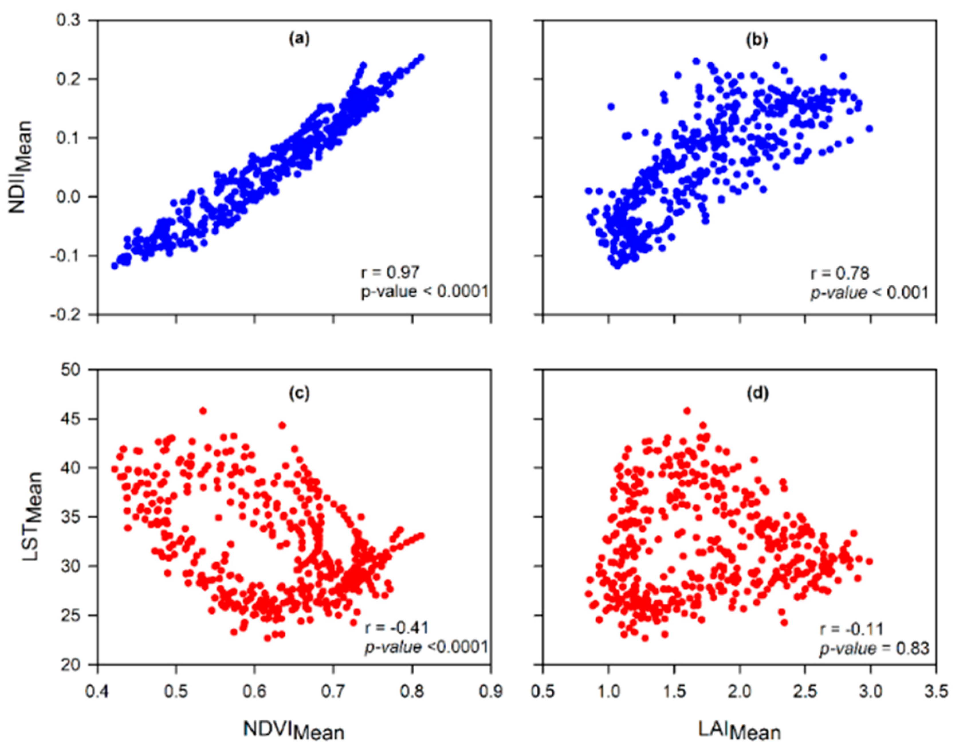
Canopy cover and water content were significantly higher during the rainy season, while canopy temperature was significantly higher during the dry season. Over the years, there appeared to be no significant difference in dry season canopy temperature. Across seasons, variations in canopy cover were more strongly associated with canopy water content than canopy temperature.
Plant water status (i.e., canopy water content), as a single variable, appeared to be a major determinant factor of the temporal variation in canopy cover across seasons, though combination with canopy temperature appeared to significantly improve accounting for variations in the canopy cover during the dry season. Based on the satellite data analyzed in this study, seasonal variations in canopy cover could be a water conservation strategy by Miombo plant species as a result of the changes in plant water availability and canopy temperature.
Type of variables used in assessing the most determinant factor of variations in canopy cover in the Miombo Woodland is important. This is because our results—based on the use of the satellite data LST and NDII as proxies for canopy temperature and canopy water content—suggest different outcomes in terms of which variable accounts for the most variations in canopy cover proxies (i.e., LAI and NDVI) compared to the studies that used air temperature and rainfall. This study found canopy water content and not temperature as the major determining factor in accounting for variations in canopy cover in the Miombo Woodland.
Satellite-based LST and NDII seem to have captured the seasonal variations in the Miombo Woodland and, therefore, they may be good indicators of plant water status in this ecosystem. However, field measurements are needed to determine the degree of correlation with actual physical conditions.

Supplementary Materials

The following are available online at https://www.mdpi.com/2306-5338/7/3/58/s1, Table S1: Dixon test results (a) cool-dry season, (b) hot-dry season, and (c) peak rainy season for the period 2009–2018, Table S2: (a–d). ANOVA statistics of variables, Table S3: (a–d). ANOVA statistics for inter-annual variations, Table S4: Pearson r correlation statistics of variables for the rainy season (November–April) for the period 2009–2018, Table S5: Pearson r correlation statistics of variables for the dry season (May–October) for the period 2009–2018, Table S6: Pearson r correlation statistics of variables for the cool-dry season (May–July) for the period 2009–2018, Table S7: Pearson r correlation statistics of variables for the hot-dry season (August–October) for the period 2009–2018, Table S8: CCR.LM coefficients of estimates and goodness of fit statistics (at 95% confidence level) during the rainy season (November–April). Combined NDII and LST interaction improved accounting for variations in LAI by 14.29% but zero% in the case of NDVI, Table S9: CCR.LM coefficients of estimates and goodness of fit statistics (at 95% confidence level) for the cool-dry season (May–July). The NDII and LST interaction did not improve accounting for variations in LAI and NDVI, Table S10: CCR.LM coefficients of estimates and goodness of fit statistics (at 95% confidence level) for the hot-dry season (August–October). The NDII and LST interaction significantly improved accounting for variations in LAI (112 percent) and NDVI (64.58 percent), Table S11: (a) Pettit homogeneity test results during the dry season for the period 2009–2018, (b). Mann–Kendall trends test results for the period 2009–2018, (c) Dry season Mann–Kendall trends test results for the period 2009–2018.

Author Contributions

Conceptualization, H.Z.; formal analysis, H.Z.; resources, H.S.; supervision, M.C.-G. and B.K.; writing—original draft, H.Z.; writing—review and editing, M.C.-G., B.K., H.S., I.N., and H.W. All authors have read and agree to the published version of the manuscript.

Funding

This research was funded by the Dutch Research Council (NWO) of the Netherlands under the project number W 07.303.102.

Acknowledgments

This study is part of the ZAMSECUR Project, whose focus is to observe and understand the remote water resources for enhancing water, food, and energy security in Lower Zambezi.

Conflicts of Interest

The authors declare no conflict of interest.

References

  1. Guumbo, J.D.; Dumas-Johansen, M.; Muir, G.; Boerstler, F.; Xia, Z. Sustainable Management of Miombo Woodlands—Food Security, Nutrition and Wood Energy; Food and Agriculture Organization of the United Nations: Rome, Italy, 2018. [Google Scholar]
  2. Frost, P. The ecology of miombo woodlands. In The Miombo in Transition: Woodlands and Welfare in Africa; Centre for International Forestry Research: Borgo, Indonesia, 1996; pp. 11–57. [Google Scholar]
  3. Pelletier, J.; Paquette, A.; Mbindo, K.; Zimba, N.; Siampale, A.; Chendauka, B.; Roberts, J.W. Carbon sink despite large deforestation in African tropical dry forests (miombo woodlands). Environ. Res. Lett. 2018, 13, 1–14. [Google Scholar] [CrossRef] [Green Version]
  4. Jew, E.K.; Dougill, A.J.; Sallu, S.M.; O’Connelle, J.; Benton, T.G. Miombo woodland under threat: Consequences for tree diversity andcarbon storage and carbon storage. For. Ecol. Manag. 2016, 361, 144–153. [Google Scholar] [CrossRef] [Green Version]
  5. Munishi, P.K.; Mringi, S.; Shirima, D.D.; Linda, K.S. The role of the Miombo Woodlands of the Southern Highlands of Tanzania as carbon sinks. J. Ecol. Nat. Environ. 2010, 2, 261–269. [Google Scholar]
  6. Sutanto, S.J.; Wenninger, J.; Coenders-Gerrits, A.M.J.; Uhlenbrook, S. Partitioning of evaporation into transpiration, soil evaporation and interception: A comparison between isotope measurements and a HYDRUS-1D model. Hydrol. Earth Syst. Sci. 2012, 16, 2605–2616. [Google Scholar] [CrossRef] [Green Version]
  7. Gerrits, A.M.J. The Role of Interception in the Hydrological Cycle; VSSD: Delft, The Netherlands, 2010. [Google Scholar]
  8. IPCC. Climate Change, Synthesis Report in Contribution of Working Groups I, II and III to the Fourth Assessment Report of the Intergovernmental Panel on Climate Change; IPCC: Geneva, Switzerland, 2007. [Google Scholar]
  9. Wegehenkel, M. Modeling of vegetation dynamics in hydrological models for the assessment of the effects of climate change on evapotranspiration and groundwater recharge. Adv. Geosci. 2009, 21, 109–115. [Google Scholar] [CrossRef] [Green Version]
  10. Chidumayo, E.N. Species structure in Zambian Miombo woodland. J. Trop. Ecol. 1987, 3, 109–118. [Google Scholar] [CrossRef]
  11. Giliba, R.A.; Boon, E.K.; Kayombo, C.J.; Musamba, E.B.; Kashindye, A.M.K.; Shayo, P.F. Species Composition, Richness and Diversity in Miombo Woodland of Bereku Forest Reserve, Tanzania. J. Biodivers. 2011, 2, 1–7. [Google Scholar] [CrossRef]
  12. Gonçalves, F.M.P.; Revermann, R.; Gomes, A.L.; Aidar, M.P.M.; Finckh, M.; Juergens, N. Tree Species Diversity and Composition of MiomboWoodlands in South-Central Angola: A Chronosequence ofForest Recovery after Shifting Cultivation. Int. J. For. Res. 2017, 2017, 6202093. [Google Scholar]
  13. Vinya, R.; Malhi, Y.; Brown, N.D.; Fisher, J.B.; Brodribb, T.; Aragão, L.E. Seasonal changes in plant–water relations influence patterns of leaf display in Miombo woodlands: Evidence of water conservative strategies. Tree Physiol. 2019, 39, 104–112. [Google Scholar] [CrossRef] [Green Version]
  14. Chidumayo, E. Climate and Phenology of Savanna Vegetation in Southern Africa. J. Veg. Sci. 2001, 12, 347–354. [Google Scholar] [CrossRef]
  15. Wulder, M.A.; Franklin, S.E. Remote Sensing of Forest Environments, Introduction. In Remote Sensing of Forest Environments; Wulder, M.A., Franklin, S.E., Eds.; Springer: Boston, MA, USA, 2003. [Google Scholar]
  16. Lechne, A.M.; Foody, G.M.; Boyd, D.S. Applications in Remote Sensingto Forest Ecology and Management. One Earth 2020, 2, 405–412. [Google Scholar] [CrossRef]
  17. Lausch, A.; Erasmi, S.; King, D.J.; Magdon, P.; Heurich, M. Understanding Forest Health with Remote Sensing—Part II—A Review of Approachesand Data Models. Remote Sens. 2017, 9, 129. [Google Scholar] [CrossRef] [Green Version]
  18. Wang, K.; Franklin, S.E.; Guo, X.; Cattet, M. Remote Sensing of Ecology, Biodiversity and Conservation: A Review from the Perspective of Remote Sensing Specialists. Sensors 2010, 10, 9647–9667. [Google Scholar] [CrossRef] [PubMed]
  19. Tian, F.; Wigneron, J.-P.; Ciais, P.; Chave, J.; Ogee, J.; Penuelas, J.; Raebild, A.; Domec, J.-C.; Tong, X.; Brandt, M.; et al. Fensholt, Coupling of ecosystem-scale plant water storage and leaf phenology observed by satellite. Nat. Ecol. Evol. 2018, 2, 1428–1435. [Google Scholar] [CrossRef] [Green Version]
  20. Botta, A.; Viory, N.; Ciais, P.; Friedlingstein, P.; Monfray, P. A global prognostic scheme of leaf onset satellite data. Glob. Chang. Biol. 2000, 6, 709–725. [Google Scholar] [CrossRef]
  21. Jeffers, J.N.R.; Boaler, S.B. Ecology of a miombo site. Lupa North Forest Reserve, Tanzania. I. Weather and plant growth, 1962-64. Ecology 1966, 54, 447–463. [Google Scholar] [CrossRef]
  22. Woodward, F.I. Temperature and the distribution of plant species. Symp. Soc. Exp. Ecol. 1988, 42, 59–75. [Google Scholar]
  23. Rouse, W.J.; Haas, R.H.; Schell, A.J.; Deering, D.W. Monitoring vegetation sytems in the great plains with ERTS. Remote Sens. Cent. 1973, 309–317. [Google Scholar]
  24. Cammalleri, C.; Vogt, J. On the Role of Land Surface Temperature as Proxy of Soil Moisture Status for Drought Monitoring in Europe. Remote Sens. 2005, 7, 16849–16864. [Google Scholar] [CrossRef] [Green Version]
  25. Dash, P.; Gottsche, F.M.; Olesen, F.S.; Fischer, H. Land surface temperature and emissivity estimation from passive sensor data: Theory and practice-current trends. Int. J. Remote Sens. 2002, 23, 2563–2594. [Google Scholar] [CrossRef]
  26. Li, Z.-L.; Tang, B.-H.; Wu, H.; Ren, H.; Yan, G.; Wan, Z.; Trigo, I.F.; Sobrino, J.A. Satellite-derived land surface temperature: Current status and perspectives. Remote Sens. Environ. 2013, 131, 14–37. [Google Scholar] [CrossRef] [Green Version]
  27. Avdan, U.; Jovanovska, G. Algorithm for Automated Mapping of Land Surface Temperature Using LANDSAT 8 Satellite Data. J. Sens. 2016, 2016, 1480307. [Google Scholar] [CrossRef] [Green Version]
  28. García-Santos, V.; Cuxart, J.; Martínez-Villagrasa, D.; Jiménez, M.A.; Simó, G. Comparison of Three Methods for Estimating Land Surface Temperature from Landsat 8-TIRS Sensor Data. Remote Sens. 2018, 10, 1450. [Google Scholar] [CrossRef] [Green Version]
  29. Hulley, G. MYD21A2 MODIS/Aqua Land Surface Temperature/3-Band Emissivity 8-Day L3 Global 1km SIN Grid V006; NASA EOSDIS Land Processes DAAC: Pasadena, CA, USA, 2017. [Google Scholar]
  30. Jones, H.G.; Rotenberg, E. Energy, Radiation and Temperature Regulation in Plants; Encyclopedia of Life Sciences; John Wiley & Sons, Ltd.: Chichester, UK, 2001; pp. 1–7. [Google Scholar]
  31. Sun, Z.; Wang, Q.; Batkhishig, O.; Relationship, Z.O. between Evapotranspiration and Land Surface Temperature under Energy- and Water-Limited Conditions in Dry and Cold Climates. Adv. Meteorol. 2016, 2016, 1–9. [Google Scholar] [CrossRef] [Green Version]
  32. Mildrexler, D.J.; Zhao, M.; Running, S.W. Aglobal comparison between station air temperatures and MODIS land surface temperatures reveals the cooling role of forests. Geophys. Res. 2011, 116, 1–15. [Google Scholar] [CrossRef]
  33. Mobasheri, M.R.; Fatemi, S.B. Leaf Equivalent Water Thickness assessment using reflectance at optimum wavelengths. Theor. Exp. Plant. Physiol. 2013, 25, 196–202. [Google Scholar] [CrossRef] [Green Version]
  34. Fensholt, R.; Sandholt, I. Derivation of a shortwave infrared stress index from MODIS near- and shortwave infrared data in a semiarid environment. Remote Sens. Environ. 2003, 87, 111–121. [Google Scholar] [CrossRef]
  35. Hardisky, M.A.; Klemas, V.; Smart, R.M. The Influence of Soil Salinity, Growth Form, and Leaf Moisture on the Spectral Radiance of Spartina alterniflora Canopies. Photogramm. Eng. Remote Sens. 1988, 49, 77–83. [Google Scholar]
  36. Hunt, J.E.R.; Rock, B.N. Detection of changes in leaf water content using near and middle-infrared reflectances. Remote Sens. Environ. 1989, 30, 43–54. [Google Scholar]
  37. Gao, B.C. NDWI—A normalized difference water index for remote sensing of vegetation liquid water from space. Remote Sens. Environ. 1996, 58, 257–266. [Google Scholar] [CrossRef]
  38. Sriwongsitanon, N.; Gao, H.; Savenije, H.H.G.; Maekan, E.; Saengsawang, S.; Thianpopirug, S. The Normalized Difference Infrared Index (NDII) as a proxy for soil moisture storage in hydrological modelling. Hydrol. Earth Syst. Sci. 2015, 12, 8419–8457. [Google Scholar] [CrossRef]
  39. Yilmaz, M.T.; Hunt, E.R., Jr.; Jackson, T.J. Remote sensing of vegetation water content from equivalent water thickness using satellite imagery. Remote Sens. Environ. 2008, 112, 2514–2522. [Google Scholar] [CrossRef]
  40. Marin, C.T.; Bouten, W.; Sevink, J. Gross rainfall and its partitioning into throughfall, stemflow andevaporation of intercepted water in four forest ecosystems inwestern Amazonia. J. Hydrol. 2000, 237, 40–57. [Google Scholar] [CrossRef]
  41. Myneni, R.; Knyazikhin, Y.; Park, T. MCD15A2H MODIS/Terra+Aqua Leaf Area Index/FPAR 8-day L4 Global 500m SIN Grid V006; NASA EOSDIS Land Processes DAAC: Missoula, MT, USA, 2015. [Google Scholar] [CrossRef]
  42. Fuller, D.O.; Prince, S.D.; Astle, W.L. The influence of canopy strata on remotely sensed observation of savannah woodlands. Int. J. Remote Sens. 1997, 18, 2985–3009. [Google Scholar] [CrossRef]
  43. Cano, E.; Denux, J.-P.; Bisquert, M.; Hubert-Moy, L.; Chéret, V. Improved forest-cover mapping based on MODIStime series and landscape stratification. Int. J. Remote Sens. 2017, 38, 1865–1888. [Google Scholar] [CrossRef] [Green Version]
  44. Reeves, M.C.; Zhao, M.; Running, S.W. Applying improved estimates of MODIS productivity of characterize grassland vegetation dynamics. Rangel. Ecol. Manag. 2006, 59, 1–10. [Google Scholar] [CrossRef]
  45. Ticehurst, C.; Guerschman, P.J.; Yun, C. The Strengths and Limitations in Using the Daily MODIS Open Water Likelihood Algorithm for Identifying Flood Events. Remote Sens. 2014, 6, 11791–11809. [Google Scholar] [CrossRef] [Green Version]
  46. García-Mora, T.J.; Mas, J.-F.; Hinkley, E.A. Land cover mapping applications with MODIS: A literature review. Int. J. Digit. Earth 2012, 5, 63–87. [Google Scholar] [CrossRef]
  47. Vermote, E.F.; Kotchenova, S.Y.; Ray, J.P. MODIS Surface Reflectance User’s Guide. Available online: http://modis-sr.ltdri.org (accessed on 11 February 2011).
  48. Didan, K.; Munoz, A.B.; Solano, R.; Huete, A. MODIS Vegetation Index User’s Guide; MOD 13 Series; The University of Arizona: Tucson, AZ, USA, 2015. [Google Scholar]
  49. Running, S.Q. MOD16A2 MODIS/Terra Net Evapotranspiration 8-Day L4 Global 500m SIN Grid V006; NASA EOSDIS Land Processes DAAC: Missoula, MT, USA, 2017. [Google Scholar]
  50. Magidson, J. Correlated Component Regression: Re-thinking Regression in the Presence of Near Collinearity. In New Perspectives in Partial Least Squares and Related Methods; Abdi, H., Chin, W., Esposito Vinzi, V., Russolillo, G., Trinchera, L., Eds.; Springer: New York, NY, USA, 2013; Volume 56. [Google Scholar]
  51. Beilfus, R.; Risky, A. Climate for Southern African Hydro: Assessing Hydrological Risks and Consequences for the Zambezi River Basin Dams; International Rivers: Berkeley, CA, USA, 2012. [Google Scholar]
  52. Timberlake, J.; Chidumayo, E. Miombo Eco-Region Vision Report; Biodiversity Foundation for Africa: Bulawayo, Zimbabwe, 2001. [Google Scholar]
  53. Miombo Network. Available online: http://www.miombonetwork.org (accessed on 30 January 2020).
  54. Saha, S.; Moorthi, S.; Wu, X.; Wang, J.; Nadiga, S.; Tripp, P.; Behringer, D.; Hou, Y.; Chuang, H.; Iredell, M.; et al. The NCEP Climate Forecast System Version 2. J. Clim. 2014, 27, 2185–2208. [Google Scholar] [CrossRef]
  55. Saha, S.; Moorthi, S.; Pan, H.; Wu, X.; Wang, J.; Nadiga, S.; Tripp, P.; Kistler, R.; Woollen, J.; Behringer, D.; et al. The NCEP Climate Forecast System Reanalysis. Bull. Am. Meteorol. Soc. 2010, 91, 1015–1057. [Google Scholar] [CrossRef]
  56. Gray, J.; Sulla-Menashe, D.; Friedl, M.A. User Guide to Collection 6 MODIS Land Cover Dynamics (MCD12Q2) Product; NASA EOSDIS Land Processes DAAC: Missoula, MT, USA, 2019. [Google Scholar]
  57. Penman, H.L. Natural evaporation from open water, bare soil, and grass. Proc. R. Soc. A Math. Phys. Eng. Sci. 1948, 193, 120–146. [Google Scholar]
  58. Monteith, J.L. Evaporation and environment. Symp. Soc. Exp. Biol. 1965, 19, 205–234. [Google Scholar] [PubMed]
  59. Miralles, D.G.; Brutsaert, W.; Dolman, A.J.; Gash, J.H. On the use of the term ‘Evapotranspiration’. Water Resour. Res. 2020, 1–8. [Google Scholar]
  60. Savenije, H.H.G. The importance of interception and why we should delete the term evapotranspiration from our vocabulary. Hydrol. Process. 2004, 18, 1507–1511. [Google Scholar] [CrossRef]
  61. Tucker, C.J. Red and Photographic Infrared Linear Combination for Monitoring Vegetation. Remote Sens. Environ. 1979, 8, 127–150. [Google Scholar] [CrossRef] [Green Version]
  62. Nielsen, D.; Miceli-Garcia, J.J.; Lyon, D.J. Canopy cover and Leaf Area Index Relationships. Agron. J. 2012, 104, 1569–1573. [Google Scholar] [CrossRef] [Green Version]
  63. Knyazikhin, Y.; Glassy, J.; Privette, L.J.; Tian, Y.; Lotsch, A.; Zhang, Y.; Wang, Y.; Morisette, T.J.; Votava, P.; Myneni, B.R.; et al. MODIS Leaf Area Index (LAI) and Fraction of Photosynthetically Active RadiationAbsorbed by Vegetation (FPAR) Product (MOD15) Algorithm Theoretical Basis Document. 1999. Available online: http://eospso.gsfc.nasa.gov/atbd/modistables.html (accessed on 30 January 2020).
  64. Wan, Z.; Hulley, S.H.G. MYD11A2 MODIS/Aqua Land Surface Temperature/Emissivity 8-Day L3 Global 1km SIN Grid V006; NASA EOSDIS Land Processes DAAC: Missoula, MT, USA, 2015. [Google Scholar]
  65. Simic, A.; Fernandes, R.; Wang, S. Assessing the Impact of Leaf Area Index on Evapotranspiration and Groundwater Recharge across a Shallow Water Region for Diverse Land Cover and Soil Properties. J. Water Resour. Hydraul. Eng. 2014, 3, 60–73. [Google Scholar]
  66. Yu, L.; Zeng, Y.; Su, Z.; Cai, H.; Zheng, Z. The effect of different evapotranspiration methods on portraying soil water dynamics and ET partitioning in a semi-arid environment in Northwest China. Hydrol. Earth Syst. Sci. 2016, 1, 975–990. [Google Scholar] [CrossRef] [Green Version]
  67. Dixon, W.J. Analysis of extreme values. Ann. Math. Stat. 1950, 21, 488–506. [Google Scholar] [CrossRef]
  68. Pearson, K. Notes on regression and inheritance in the case of two parents. Proc. R. Soc. Lond. 1895, 58, 240–242. [Google Scholar]
  69. Helsel, D.R.; Hirsch, R.M. Statistical Methods in Water Resources. In Hydrologic Analysis and Interpretation; U.S. Geological Survey: Washington, WA, USA, 2002; pp. 1–524. [Google Scholar]
  70. Cirillo, M.; Poli, A.A. On the use of the Normalised Mean Square Error in evaluating dispersion model performance. Atmos. Environ. 1993, 27, 2427–2434. [Google Scholar]
  71. Pettit, A.N. A non-Parametric approach to the change-point problem. J. R. Stat. Soc. Ser. C Appl. Stat. 1979, 28, 126–135. [Google Scholar] [CrossRef]
  72. Zimba, H.; Banda, K.; Anthony, C.; Wilson, P.; Peter, S.; Markus, M.; Imasiku, N. Assessment of trends in inundation extent in the Barotse Floodplain, upper Zambezi River Basin: A remote sensing-based approach. J. Hydrol. Reg. Stud. 2018, 15, 149–170. [Google Scholar] [CrossRef]
  73. Kendall, M.G. Rank Correlation Measures; Charles Griffin: London, UK, 1975. [Google Scholar]
  74. Mann, H.B. Nonparametric test against trend. Econometrica 1945, 13, 245–259. [Google Scholar] [CrossRef]
  75. Sens, P.K. Estimates of the regression coefficient based on Kendall’ Tau. Am. Stat. Assoc. 1968, 63, 1379–1389. [Google Scholar]
  76. Salmi, T.; Määttä, A.; Anttila, P.; Ruoho-Airola, T.; Amnell, T. Detecting Trends of Annual Values of Atmospheric Pollutants by the Mann-Kendall Test and the Sens’ Slope Estimates: The Excel Template Application Makesens; Finnish Meteorological Institute: Helsinki, Finland, 2002. [Google Scholar]
  77. Fuller, D.O. Folia Phenology of Vegetation in South Central Africa and Its Relevance to Climate Change. Ph.D. Thesis, The University of Maryland, College Park, MD, USA, 1994. [Google Scholar]
  78. Ernst, W. Variation in the mineral content of leaves of trees in miombo woodland in South Central Africa. J. Ecol. 1975, 63, 801–807. [Google Scholar] [CrossRef]
  79. Johnson, J.M.; Choinski, J.S. The spring flush in Zimbabwe’s miombo woodland. Zimb. Sci. News 1993, 27, 3–6. [Google Scholar]
  80. Delogu, E.; Boulet, G.; Olioso, A.; Garrigues, S.; Brut, A.; Tallec, T.; Demarty, J.; Soudani, K.; Lagouarde, J.-P. Evaluation of the SPARSE Dual-Source Model for PredictingWater Stress and Evapotranspiration from Thermal Infrared Data over Multiple Crops and Climates. Remote Sens. 2018, 10, 806. [Google Scholar] [CrossRef] [Green Version]
  81. Karnieli, A.; Agam, N.; Pinker, R.T.; Anderson, M.; Imhoff, M.L.; Gutman, G.G.; Panov, N.; Goldberg, A. Use of NDVI and Land Surface Temperature for Drought Assessment: Merits and Limitations. J. Clim. 2010, 23, 618–633. [Google Scholar] [CrossRef]
  82. Baldocchi, D.D.; Xu, L.; Kiang, N. How plant functional-type, weather, seasonal drought, and soil physical properties alter water and energy fluxes of an oak-grass savanah and annual grassland. Agric. For. Meteorol. 2004, 123, 13–39. [Google Scholar] [CrossRef] [Green Version]
  83. Vinya, R.; Malhi, Y.; Fisher, J.B.; Brown, N.; Brodribb, T.J.; Aragao, L.E. Xylem cavitation vulnerability influences tree species’ habitat preferences in Miombo woodlands. Oecologia 2013, 173, 711–720. [Google Scholar] [CrossRef] [PubMed]
  84. Jaafar, S.W.M.W.; Maulud, K.N.A.; Kamarulzaman, M.A.M.; Raihan, A.; Sah, S.M.; Ahmad, A.; Saad, M.S.N.; Azmi, A.T.M.; Syukri, N.K.A.J.; Khan, W.R. The Influence of Deforestation on Land Surface Temperature—A Case Study of Perak and Kedah, Malaysia. Forests 2020, 11, 670. [Google Scholar] [CrossRef]
Figure 1. Extent of the Miombo Woodland in sub-Sahara Africa and the Luangwa sub-basin of the Zambezi River Basin showing the Miombo Woodland study location in Zambia. The studied Miombo Woodland is located within the central Zambezian Miombo Woodland, which is the largest Miombo subgroup. Map of Miombo Woodland adapted from the Miombo network [53]. Land cover map was adapted/based on the 2018 Copernicus global land cover map for Africa.
Hydrology 07 00058 g001
Figure 2. Phenology calendar at the Miombo Woodland site in Mpika, Zambia based on the data for the period 2009 to 2017. Shaded box indicates the dry season.
Hydrology 07 00058 g002
Figure 3. Illustration of (a) seasonal pattern in 8-day mean values of canopy cover (i.e., LAI and NDVI), canopy water content (i.e., NDII), and canopy temperature (i.e., LST). (b) Seasonal pattern in 8-day mean values of actual evaporation (Ea). Shaded area for variables is the 5th and 95th percentiles. The shaded area (grey) is the dry season. The rainy and dry season seasons are clearly delineated with peak values in Ea, LAI, NDII, and NDVI observed during the rainy season while lowest values were observed in the dry season. Peak canopy temperature (i.e., LST) value(s) were observed during the dry season. Ea = Actual evaporation, LAI = Leaf area index, LST = Land surface temperature, NDII = Normalised difference infrared index and NDVI = Normalised difference vegetation index.
Hydrology 07 00058 g003
Figure 4. 2009–2018 January to December minimum (a) and maximum (b) values of Ea, LAI, NDII, and NDVI. Lowest values were seen during the dry season while peak values were observed in the rainy season. Shaded areas represent the rainy season: November–December indicate start of the rainfall, January–February is the peak rainfall period, while March–April is the end of the rainfall season.
Hydrology 07 00058 g004
Figure 5. Correlation of mean values for the 8-day NDVIMean and LAIMean with NDIIMean (a,b), as well as with LSTMean (c,d) at the annual scale. The NDVIMean shows stronger correlation with canopy water content (i.e., NDII) and canopy temperature (i.e., LST) compared to the LAIMean when used as proxies for canopy cover. LSTMean shows hysteresis with NDVIMean and LAIMean while NDIIMean shows hysteresis with LAIMean.
Hydrology 07 00058 g005
Figure 6. First row: Plots of the CCR.LM results at annual scale (January–December) (a,b) and dry season (May–October) (c,d): LAI regression graphs at annual scale (a) with NDII as only predictor variable and (b) with LST and NDII used simultaneously as predictors. LAI regression graphs during the dry season (c) with NDII as only predictor variable and (d) with LST and NDII combined as predictor variables. Second row: Plots of the CCR.LM results at annual scale (January–December) (a,b) and dry season (May–October) (c,d): NDVI regression graphs at annual scale (a) with NDII as only predictor variable and (b) with LST and NDII combined as predictors. NDVI regression graphs during the dry season (c) with NDII as only predictor variable and (d) with LST and NDII used simultaneously as predictor variables. R2 = coefficient of determination, BN = unstandardized coefficient of estimate with the NDII, BL = unstandardized coefficient of estimate with the LST, i = intercept, N = number of observations.
Hydrology 07 00058 g006
Figure 7. Plots of the Pettit test for the 8-day LSTMin (a), LSTMax (b), LSTMean (c), NDIIMax (d), NDVImax (e), and mean annual rainfall (f) for the period of 2009 to 2018 in the Miombo Woodland in the Luangwa Basin. Significant upward change in the LST means seemed to have occurred in August 2012. Significant abrupt changes in NDIIMax and NDVIMax seem to have occurred in May at the start of the dry season.
Hydrology 07 00058 g007
Figure 8. Mann–Kendall trends test and the Sens’ slope estimates for mean annual rainfall (a), mean annual LAIMean (b), mean annual NDIIMean (c), mean annual NDVIMean (d), and mean annual LSTMean (e) for the period of 2009 to 2018. Years with relatively high LST values seem to correspond to years with relatively low rainfall and NDII values.
Hydrology 07 00058 g008
Table 1. Characteristics of the moderate resolution imaging spectroradiometer (MODIS) terra/aqua surface reflectance data [47]. NIR = Near infrared and SWIR = Shortwave infrared.
Band No.Visible RangeBand Centre (nm)Wavelength Range (nm)Resolution (m)Key Applications
B01Red648620–670500Absolute land cover transformation, vegetation chlorophyll
B02NIR-1858841–876500Cloud amount, vegetation, land cover transformation
B03Blue470459–479500Soil/vegetation differences
B04Green555545–565500Green vegetation
B05NIR-212401230–1250500Leaf/canopy differences
B06SWIR-116401628–1652500Snow/cloud differences
B07SWIR-221302105–2155500Cloud properties, land properties
Table 2. Repeated measure-analysis of variance(RM-ANOVA) test results for variables.
Rainy Season vs. Dry SeasonDry Season Inter-Annual Variations
VariableMean DiffDFFp-ValueDFFp-Value
LAIMean2.32(1,454)596.62<0.001(9,198)9.41<0.001
LSTMean2.48(1,438)20.87<0.001(9,197)0.590.805
NDIIMean0.15(1,458)485.12<0.001(9,192)11.27<0.001
NDVIMean0.13(1,454)306.70<0.001(9,192)7.96<0.001
Mean Diff = Mean difference, DF = Degree of freedom, F = Test statistic.
Table 3. Pearson (r) correlation statistics of the minimum, maximum, and mean values of LAI, LST, NDII, and NDVI at an annual scale. The LST minimum values showed relatively stronger correlation with minimum values of LAI, NDII, and NDVI compared to the maximum and mean values.
VariableLSTMinLSTMaxLSTMeanNDVIMinNDVIMaxNDVIMeanNDIIMinNDIIMaxNDIIMeanLAIMinLAIMaxLAIMean
LSTMin1.000.940.97−0.51−0.38−0.50−0.42−0.24−0.37−0.12−0.02−0.08
LSTMax 1.000.99−0.43−0.31−0.41−0.33−0.14−0.26−0.110.100.01
LSTMean 1.00−0.43−0.31−0.41−0.33−0.15−0.27−0.110.090.01
NDVIMin 1.000.900.980.970.860.940.350.580.69
NDVIMax 1.000.940.920.930.940.360.620.72
NDVIMean 1.000.960.890.970.350.610.71
NDIIMin 1.000.920.970.340.650.75
NDIIMax 1.000.960.360.700.78
NDIIMean 1.000.350.690.78
LAIMin 1.000.200.51
LAIMax 1.000.79
LAIMean 1.00
Interpretation: Min = Minimum, Max = Maximum. Values in bold are different from 0 with a significance level alpha = 0.05.
Table 4. CCR.LM coefficients of estimates and goodness of fit statistics (at 95% confidence level) at annual scale with NDII and LST as predictors. Accounting for variations in LAI was improved by about 9.83% when LST and NDII were simultaneously inputted as predictors. Accounting for variations in NDVI improved by 3.22% when LST and NDII were simultaneously used as predictors.
LSTNDIIPredictors—NDII and LST
Model
ModelGFS CvModelGFS CVLSTNDIIGoodness of Fit Statistics CVChange
Variable β ^ iR2NMSE β ^ iR2NMSEN β ^ β ^ iR2NMSENDiff. R2(%)
LAI−0.0011.690.130.874.691.460.610.394350.035.150.610.670.334350.069.83
NDVI−0.010.870.170.831.020.570.930.07435−0.0030.970.670.960.044350.093.22
Table 5. CCR.LM coefficients of estimates and goodness of fit statistics (at 95% confidence level) during the dry season with NDII and LST as predictors. Accounting for variations in LAI was improved by about 46% when LST and NDII were simultaneously used as predictor variable.
LSTNDIIPredictors—NDII and LST
Model
ModelGFS CvModelGFS CVLSTNDIIGoodness of Fit Statistics CVChange
Variable β ^ iR2NMSE β ^ iR2NMSEN β ^ β ^ iR2NMSENDiff. R2(%)
LAI0.0011.280.210.792.921.340.560.442050.034.290.50.820.182050.2646.43
NDVI−0.010.890.560.441.180.570.900.16205−0.0040.930.710.960.042050.116.67
Interpretation (Table 2 and Table 3): GFS Cv = Goodness of fit statistics cross validated, i = intercept, N = number of observations, NDVI = Normalized difference vegetation index, LST = Land surface temperature, LAI = Leaf area index, NMSE = Normalized mean square error, R2 = coefficient of determination, and β ^ = unstandardized coefficient of estimate.
Table 6. Pettit test results for LAI, LST, NDII, and NDVI for the period 2009–2018 for study area.
VariablePeriodChange TimeYearp-ValueAlpha LevelConf. LevelMean fromMean toTest Decision
LAIMin2009–2018 0.54630.0599% p > α, H0 accepted
LAIMax2009–2018 0.61270.0599% p > α, H0 accepted
LAIMean2009–2018 0.54200.0599% p > α, H0 accepted
LSTMin2009–20184th August20120.00270.0599%28.330.04p < α, H0 rejected
LSTMax2009–201812th August2012<0.00010.0599%32.7935.59p < α, H0 rejected
LSTMean2009–201812th August2012<0.00010.0599%30.532.8p < α, H0 rejected
NDIIMin2009–2018 0.07980.0599% p > α, H0 accepted
NDIIMax2009–201816th May20160.00040.0599%0.050.01p < α, H0 rejected
NDIIMean2009–2018 0.09420.0599% p > α, H0 accepted
NDVIMin2009–2018 0.05730.0599% p > α, H0 accepted
NDVIMax2009–20189th May20100.02870.0599%0.620.56p < α, H0 rejected
NDVIMean2009–2018 0.14960.0599% p > α, H0 accepted
Annual *R2009–2018 0.31620.0599% p > α, H0 accepted
Monthly *R2009–2018 0.82830.0599% p > α, H0 accepted
Daily *R2009–20124th April20120.00350.0599%4.983.90p < α, H0 rejected
Daily *R2012–201422nd April2014<0.00010.0599%6.143.65p < α, H0 rejected
Daily *R2014–201615th November2016<0.00010.0599%2.485.07p < α, H0 rejected
* R = rainfall.
Table 7. Mann–Kendall trends test results for variables with abrupt change points.
VariableMann–Kendall Statistic (S)Kendall’s TauVar (S)p-ValueAlphaTest InterpretationNature of Trend
LSTMin86420.081910,850,159.330.00870.05Reject H0Upward
LSTMax93050.088210,850,163.670.00470.05Reject H0Upward
LSTMean97090.09210,850,179.670.00320.05Reject H0Upward
NDIIMax−10,094−0.095610,850,248.000.00220.05Reject H0Downward
NDVIMax−7748−0.073410,850,248.000.01870.05Reject H0Downward
* Rainfall 2009–2018−86,112−0.01474,830,751,280.000.21540.05Accept H0No trend
* Rainfall 2012–2018−86,394−0.03851,143,571,362.000.01060.05Reject H0Downward
* Rainfall 2014–201878,2360.0614492,345,124.000.00040.05Reject H0Upward
* Rainfall 2016–201877,7110.0609493,326,659.670.00050.05Reject H0Upward
Annual rainfall9.00000.2000125.00000.47430.05Accept H0No trend
Monthly rainfall1820.0263191,454.670.67910.05Accept H0No trend
* Rainfall = daily rainfall values used.

