Long-Term Groundwater Level Prediction Model Based on Hybrid KNN-RF Technique

Abstract

Reliable seasonal prediction of groundwater levels is not always possible when the quality and the amount of available on-site groundwater data are limited. In the present work, a hybrid K-Nearest Neighbor-Random Forest (KNN-RF) is used for the prediction of variations in groundwater levels (L) of an aquifer with the groundwater relatively close to the surface (<10 m) is proposed. First, the time-series smoothing methods are applied to improve the quality of groundwater data. Then, the ensemble K-Nearest Neighbor-Random Forest (KNN-RF) model is treated using hydro-climatic data for the prediction of variations in the levels of the groundwater tables up to three months ahead. Climatic and groundwater data collected from eastern Rwanda were used for validation of the model on a rolling window basis. Potential predictors were: the observed daily mean temperature (T), precipitation (P), and daily maximum solar radiation (S). Previous day’s precipitation P (t − 1), solar radiation S (t), temperature T (t), and groundwater level L (t) showed the highest variation in the fluctuations of the groundwater tables. The KNN-RF model presents its results in an intelligible manner. Experimental results have confirmed the high performance of the proposed model in terms of root mean square error (RMSE), mean absolute error (MAE), Nash–Sutcliffe (NSE), and coefficient of determination (R²).

1. Introduction

Groundwater is the most critical source of fresh water that serves about one-third of the world’s water demands. Socio-economic development is closely linked with the availability and accessibility of groundwater resources [1]. For instance, 36% of the domestic freshwater supply, 42% of water for agriculture, and 27% of the industrial water demand come from groundwater [2,3,4,5]. While the world’s water demand is expected to rise significantly in the future [6], recent studies report an intensive drop in groundwater levels in many parts of the world [7,8,9,10]. Human behavior and the impact of climate change are considered to be the root cause of this [11,12,13]. Nevertheless, the levels of the water tables may also fluctuate seasonally due to the amount of evapotranspiration extracts, hydraulic properties, and other natural events [14,15,16]. Also, diminished precipitation and high temperature can also lead to reduced groundwater levels during dry periods [15]. The increased dependence on groundwater, spatial-temporal variation, and discrepancies of groundwater resources have also impacted ground water levels [6,12,17,18]. This is more evident in sub-Saharan Africa (SSA) where the hydroclimate variability and droughts pose a real challenge to scientists [19]. The intense droughts are having a long-lasting economic impact on the livelihoods of people in sub-Saharan Africa [20].

Despite the high potential of groundwater for socio-economic development in sub-Saharan Africa, there has been little attention paid to this precious resource [21,22,23]. There has been limited data and groundwater research done in sub-Saharan Africa [21], and it is, therefore, very important to increase research on SSA groundwater [21,23]. Rwanda, an East African country, has been experiencing seasonal groundwater scarcity [24,25,26,27], with the eastern province the most susceptible to drought due to their reliance on groundwater as the main source of fresh water [26,27]. It is also projected that eastern Rwanda will probably face prolonged droughts in the future [26]. Little is known about the situation of groundwater resources in Rwanda [24,26,27]. Sensible decision making for water management requires timely, reliable, and actionable information. Improving methods for a precise seasonal forecast of the changing groundwater levels is a strategy towards improving the management of groundwater resources [6,15,28,29,30].

Advancements in computer modeling, computing power, and information processing have resulted in improved and practical tools for better understanding highly complex natural systems. A large amount of work has been focused on the applicability of machine learning methods to the science of hydrology. Machine learning methods have been proven in their relevance to groundwater studies [31]; however, no single technique is utilized as the available data and scenario will determine the most suitable method for a problem at hand [32]. Many of the methods described in the literature are not suited for sparse and noisy samples [33,34]. Therefore, this study intends to examine the capacity of the KNN-RF ensemble model for the characterization of seasonal responses of the groundwater levels of a permeable fractured aquifer in eastern Rwanda utilizing limited site-data. The remainder of this article is organized as follows: Section 2 elucidates related research, and Section 3 explains the study area and data preparation. The research methodology is outlined in Section 4, while research results and discussion and conclusions are provided in Section 5 and Section 6, respectively.

2. Related Work

Machine learning (ML) based approaches to hydrological modeling are an important area of research. These models are more suited to water resources studies than physical models [30,31]. The simplicity and accuracy of ML is by far better than other models [31,35,36,37]. The most common methods for prediction of groundwater resources are the artificial neural network (ANN) [35,36,38,39,40,41,42], the support vector machine (SVM) [43,44,45,46,47], and feature similarity-based approaches such as K-nearest neighbor (KNN) [48]. Nearest neighbor can also be applied with noisy samples [49]. A broad analysis of the application of ANN to the modeling of water resources is presented in the report shared by the ASCE Task force committee [37]. Zhou et al. [50] report a comparative study on ANN and SVM for the modeling of water table depths. The scholars employed discrete wavelets in data preparation, and their results suggest that SVM has higher accuracy scores than the ANN model. Similarly, the SVM method is reported to have a relatively higher score than the adaptive neuro-fuzzy inference system and the ANN [51,52]. Additionally, Natarajan et al. [53] assessed the accuracy of SVM, extreme learning (ELM), genetical programming (GP), and ANN in the simulation of groundwater levels. Their finding suggests that ELM achieves higher precision than GP, SVM, and ANN. A thorough elucidation of the usage of SVM in hydrology can be found in [54,55,56]. The most recent research examines the efficiency of a non-linear auto-regressive network with exogenous input (NARX) in modeling variations of the heights of the water table using precipitation and temperature data [57,58,59]. Wunsch et al. [57] and Guzman et al. [58] reported a high performance of NARX in seasonal predictions of groundwater depths for different types of aquifers, whilst Guzman et al. [59] recommend SVM over NARX for the forecast of daily levels.

Random forest (RF) is another ensemble method for the efficient and effective representation of variations in groundwater levels. RF can efficiently handle both small as well as big datasets [60,61,62]. It is one of the most effective data-driven supervised simulation methods that does not overfit the datasets for the modeling of hydrology systems [63,64,65,66]. RF has a small number of parameters to tune; this decreases the pre-processing effort and results in faster computation, which is potent in the water resources application [65,67]. Wang et al. [60] performed short-term forecasting of groundwater levels in data-scarce areas using enhanced random forest. The scholars infused random features with RF to promote the forecasting skill of the model based on temperature and precipitation data. An enlightening discussion of the application of random forest in hydrology is found in a study by Tyralis et al. [66]. In an effort to boost the accuracy of ML models, some studies have attempted to combine multiple techniques. For example, a hybrid method combining ANN, SVM, and adaptive fuzzy inference for the simulation of groundwater levels is discussed in [51,52]. Combining multiple techniques can also boost the predictive competence of ML methods in the presence of limited input data [68,69]. A review of the literature indicates that little research has been done on the seasonal prediction of fluctuations of the groundwater tables. Most studies on the prediction of groundwater levels have focused their attention on short-term predictions. It is more important to deal with acute groundwater periods rather than focusing on annual averages [15]. A small number of studies that have examined the seasonal forecast of groundwater table variations are not designed nor suitable for the SSA environment. Many of the approaches discussed in the literature require extensive and noise-free data for reliable predictions [33]. More effective data-driven forecasting models are crucial for the quantification of groundwater resources [51].

In the study, we employ ensemble KNN-RF with time series preprocessing to predict seasonal variations of the levels of groundwater tables in a data-scarce environment. RF and KNN are non-complex, powerful methods that work efficiently in regression problems when trained using a sufficient number of training examples [65,67,70]. The nearest neighbor technique competently identifies decisive areas in the input data, but with limited training examples, the model may underperform on unseen data. While the greediness nature of RF might cause sub-optimal results for some types of data (i.e., sparse data) [70], randomized trees enhance generalization and overcome the over-fitting issue in the small datasets [71,72]. Provided with limited and noisy examples, we harness the merits of both techniques by combining them in a hybrid manner. By combining approaches the research: (1) Devises and examines the performance of the KNN-RF ensemble scheme under a limited data setting, (2) Characterizes the seasonal response of the permeable fractured aquifer in a temperate region with limited groundwater studies, and (3) Contrasts the proposed KNN-RF model with conventional groundwater modeling techniques (SVM, RF, KNN, and ANN). This study will offer the first ML-based seasonal approximation of groundwater level in Rwanda. The study will also provide new insights about the capacity of the novel KNN-RF approach for sub-Saharan semi-arid conditions.

3. Case Study and Data Processing

This section discusses the characteristics of the area under investigation, the sources, the nature of the research data, the preparation of the data, and the evaluation metrics used for the current exploration.

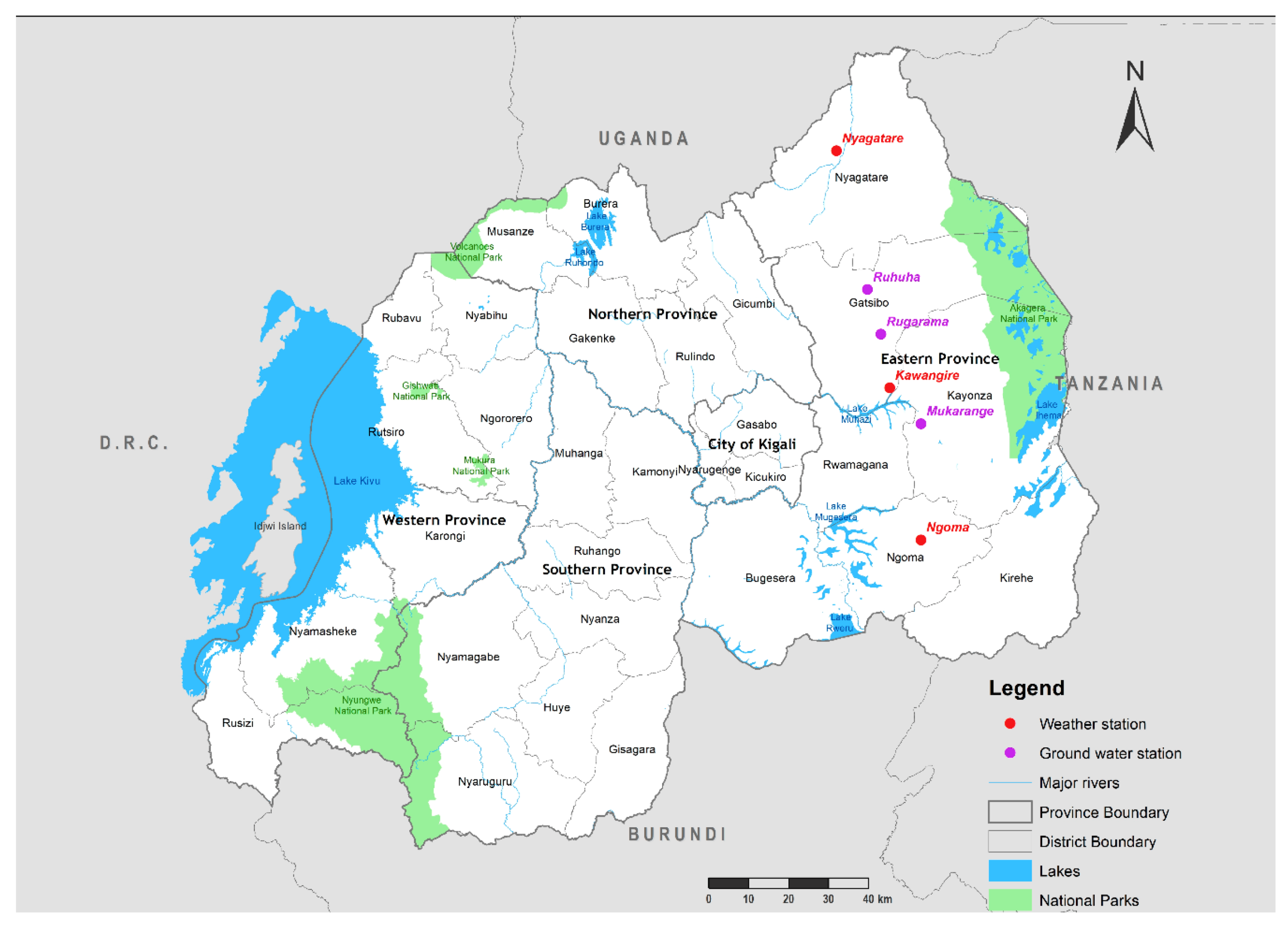
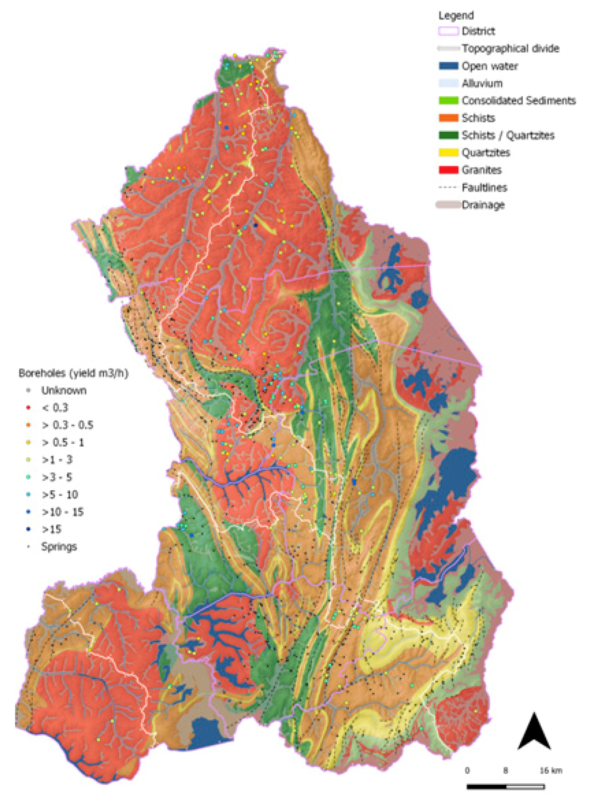
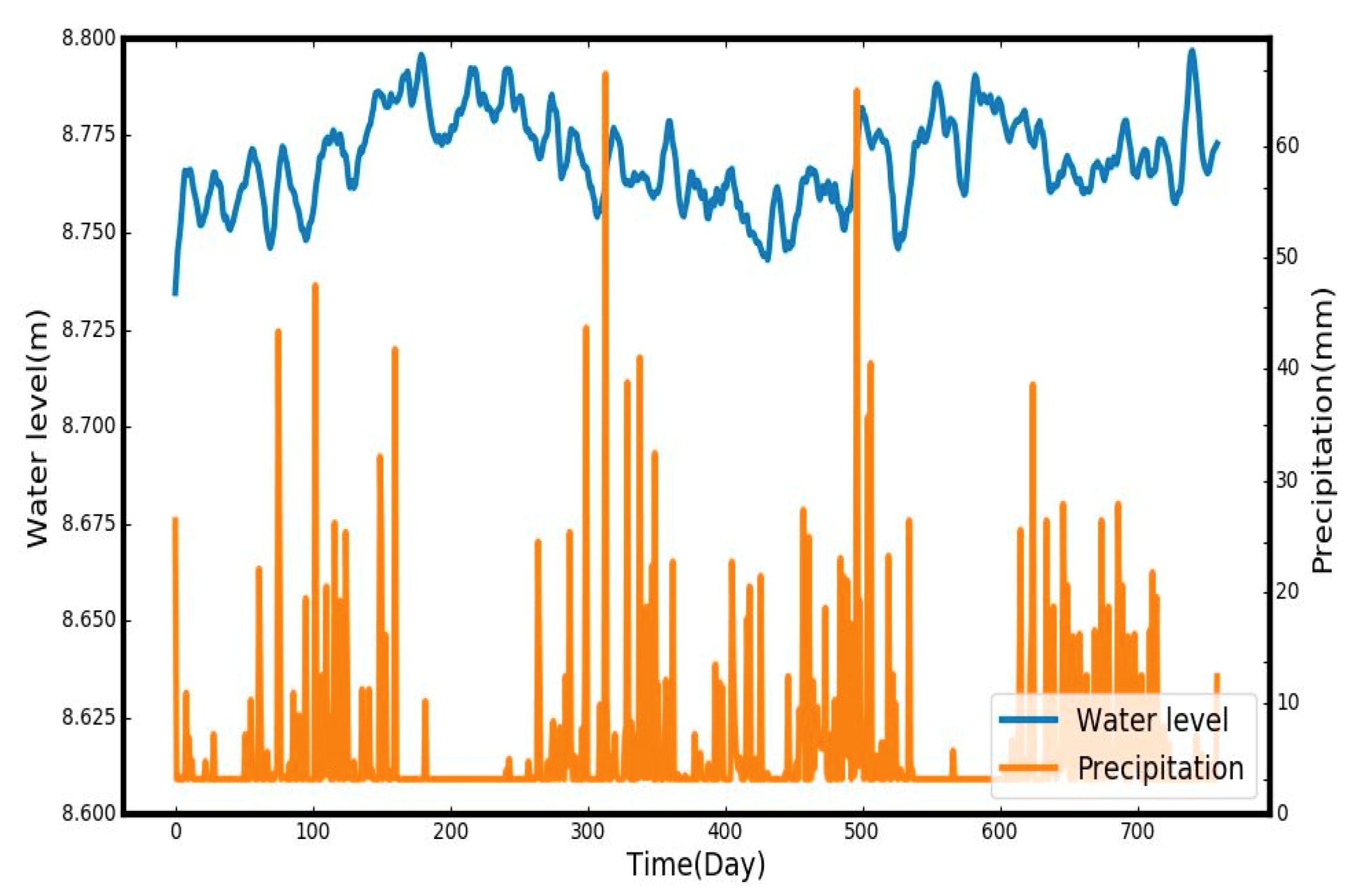
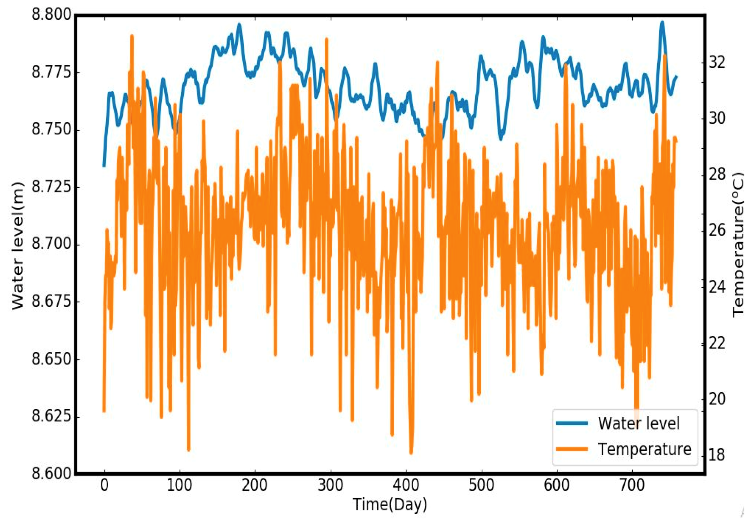
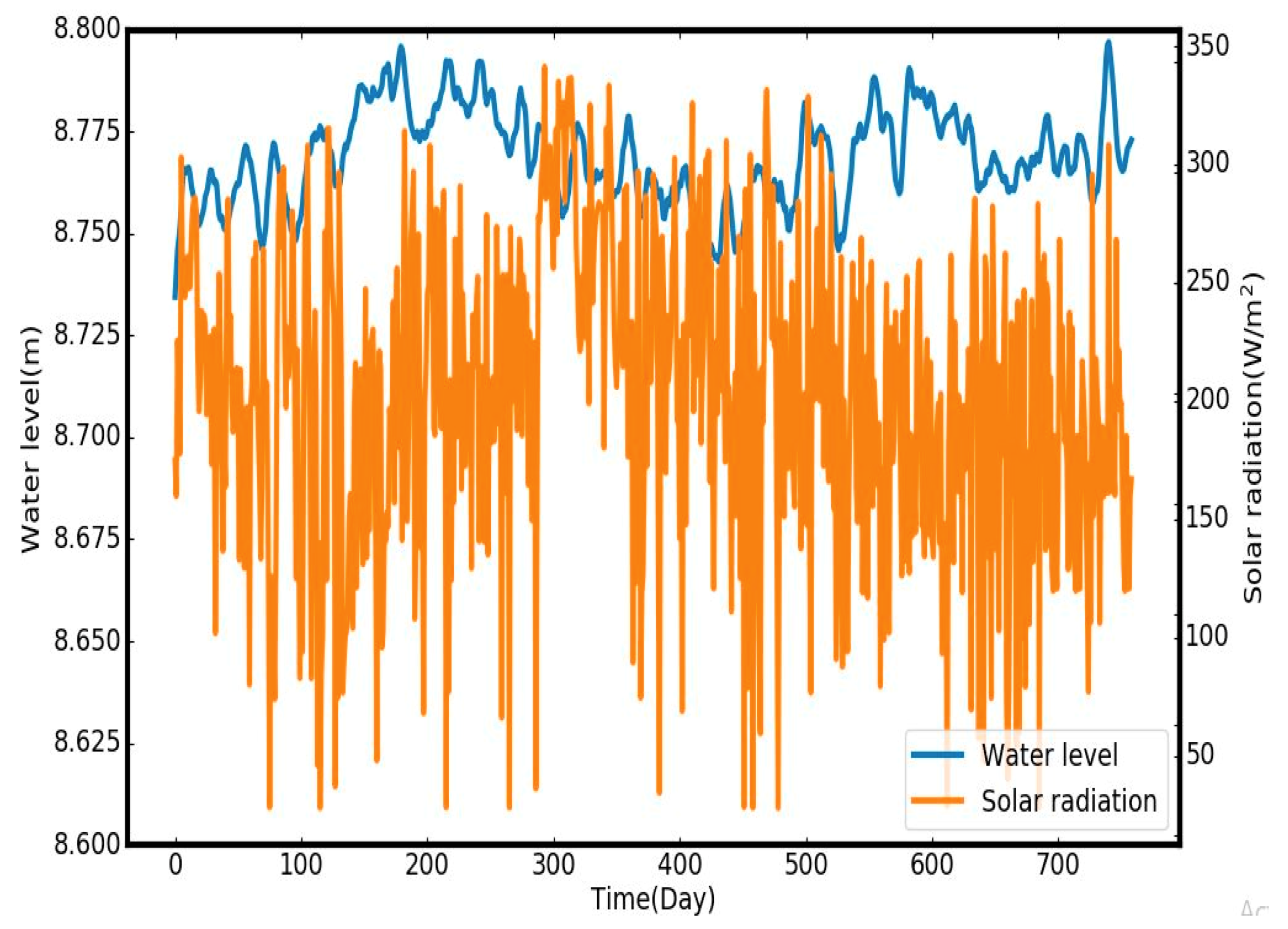
3.1. Study Area and Data

The investigated well is found in eastern Rwanda, which lies between 29.86875E–29.90625E and 2.30625S–2.26875S with a total area of 9813 ${\mathrm{km}}^2$ (3789 sq mi). This region is relatively flat with the altitude ranging between 1000 and 1500 m [73]. During the study period between December 2016 and December 2018, the majority of the rain showered in the wet season between March and May (90%), with rainfall ranges between 450 mm and 500 mm. This is less than when compared to other parts of the country, that receive on average between 600 mm and 800 mm annually [74]. The eastern province is characterized by the highest evapotranspiration rate in Rwanda. The average annual temperature varies between $15.70 °\mathrm{C}$ and $24.20 °\mathrm{C}$. The average minimum temperatures ($13 °\mathrm{C}$–$16.65 °\mathrm{C}$) are recorded in May and June, while the maximum average temperatures ($24.3 °\mathrm{C}$–$30.3 °\mathrm{C}$) are recorded in July and September [74]. The eastern province is the most populated area in Rwanda [75], and is heavily reliant on groundwater as a source of fresh water. The groundwater abstraction rate is $742{ \mathrm{m}}^3$/h, while the demand is estimated to be between 3069 and $7672{ \mathrm{m}}^3$/h [76]. This area has highly heterogeneous types of aquifers. Those aquifers range from low permeable fractured (schist), which is located in Rugarama; permeable fractured (quartzite) located in Mukarange; and fractured (granite), which is found in Ruhuha. The Rwanda Water and Forestry Authority (RWFA) has groundwater stations in each of those three aforementioned areas. A summary of the monitoring well and its features are shown in Table 1.

Table 1. Summary of the selected monitoring well and its main features.

Station ID	Name	Latitude	Longitude	Aquifer	Availability of Data	Data Time Resolution
F6	Kayonza-Mukarange	1.89874154	30.5065299	Permeable Fractured	3 December 2016–30 December 2018	Daily

Groundwater data for 2016, 2017, and 2018 were gathered from the Rwanda Water and Forestry Authority (RWFA). Weather records (precipitation, solar radiation, and temperature) are available for a longer period, and researchers decided to use only data matching to the observational period of the groundwater level. Weather data (precipitation, solar radiation, and temperature) for the period of two years, from 3 December 2016, to 30 December 2018, were obtained from nearby weather stations (Kawangire, Kibungo, and Nyagatare) that are operated by the Rwanda meteorological agency (Meteo-Rwanda). Temperature is a daily minimum and maximum observed metric measured in Celsius, daily precipitation is recorded in millimeters, while groundwater level is measured in centimeters obtained from two measurements of groundwater depth per day. For consistency reasons, the groundwater unit was converted into meters. Solar radiation is measured in watt per meter square ($W/m$) and is included in the study because it influences the evaporation and evapotranspiration [77]. The locations of the groundwater and weather stations in the case study are depicted in Figure 1.

Figure 1. Map of Rwanda shows the location of the groundwater monitoring wells and weather stations in the eastern province.

The eastern province has the highest number of boreholes and shallow wells in Rwanda. Generally, the eastern part has high-localized fractured aquifers with moderate groundwater yields, as represented in Figure 2. Alluvium based aquifers are mostly connected to fast-flowing rivers. These aquifers exhibit high groundwater potential in the eastern province [76]. The studied aquifer (Mukarange) is made of quartzite rocks fused on a schist base with a relatively high yield.

Figure 2. Eastern Province, Rwanda. Map shows hydrogeological features of the study area [76].

3.2. Data Preparation

The state of the input data is one of the key factors that determines the level of accuracy of ML-based predictions. Preprocessing and rectification of the variables ensure that all features receive equal attention throughout the training process [17,59,78]. A total of 759 daily observations from each of the above-mentioned stations were analyzed and prepared before application to the designated task [79]. Water level data were available on 12 h intervals and precipitation and temperature data were on a 24 h basis. In order to set common time intervals, we converted temperature and levels to daily averages. Data preparation was carried out with Python (3.6.6) programming language using Pandas, Numpy, Matplotlib, and SciPy data analysis libraries [80]. The RF, SVR, ANN, KNN, and KNN-RF models for prediction of groundwater levels were also realized in Python using the Scikit-Learn machine learning library (version 0.20) [81].

Water level data were available between 3 December 2016, and 30 December 2018. Weather data, including precipitation, temperature, and solar radiation data between 2010 and 2018 were acquired, and weather data between December 2016 and December 2018 that correlated to the water level data were utilized in the experiment. Evapotranspiration is one of the key factors that influence groundwater level oscillations [17]. Since evapotranspiration data were not available, solar radiation data were successfully substituted instead, as suggested in [82,83]. Temperature and groundwater level (GWL) data were converted to mean values to reduce variance among data points as recommended by [84,85]. During the analysis of the data, it was discovered that groundwater data had irregular patterns. Then, the time-series data filtering method was also used to improve the quality of that data. The exponential weighted moving average (rolling mean) produced a superior output of the groundwater level samples. This not only filtered the data, but also revealed long term trends from the data. The exponential rolling mean of a sequence $S=\left(x_1,x_2,\dots ,x_k\right)$, is:

$$S_k=a\sum _{j=1}^k{\left(1-\alpha \right)}^{j}x\left[k-j\right],$$

(1)

$$\alpha =1/\left(1+idc\right),idc\ge 0,$$

(2)

where $S_k$ is the filtered data, $k$ is the size of $S$, $\alpha$ is the decay in the interval $\left[0,1\right]$, $idc$ is the initial value of the decay, and $x$ is the input data. As the exponential weighted average is enumerated, the decay $\alpha$ value decreases exponentially in such a way the most recent observations are assigned higher weights than the old ones. For a proper scaling of the time-series data, for each stage, the features ($X_j$) were converted in the range between −1 and 1 with the formula:

$$X_s=\frac{X_j-X_{mean}}{2X_{max}}$$

(3)

where $X_s$ stands for standardized value, and $X_{max}$ and $X_{min}$ are the maximum value and minimum value of the features to be scaled, respectively. Despite the effort made to improve the samples, data from two of the observation boreholes (Ruhuha and Rugarama) were found to be unusable. Only data from one borehole (Mukarange) with 759 observations was considered for the current investigation. The groundwater level data were matched with weather data recorded in the same time period (2016–2018) from the nearby station located between −1.81 latitude and 30.43 longitude in Kawangire. The useful preprocessed dataset is shown in the pair-wise plots in Figure 3, Figure 4 and Figure 5. The time lagged water table predictors have great positive effects on the estimated levels [86]. Therefore, smoothed Mukarange data were then converted into four day time lags ($t-1$, $t-2$, $t-3$, and $t-4$) for better comparison of all the models. More details are provided in the methodology section.

Figure 3. Time series plot of precipitation and groundwater level collected from the Mukarange monitoring borehole.

Figure 4. Time series plot of temperature and groundwater level collected from the Mukarange monitoring borehole.

Figure 5. Time series plot of solar radiation and groundwater level collected from the Mukarange monitoring borehole.

From Figure 3, Figure 4 and Figure 5, it is quite clear that in dry periods (June–August and January–February) there are noticeable declines in groundwater level (GWL), during the study interval (December 2016 to December 2018). This could be connected to the higher evaporation rate, reduced replenishment, and increased groundwater withdrawals due to excessive temperatures in the studied area. Conversely, higher GWLs are observed during wet periods (March–May and September–December), which can be attributed to increased groundwater restoration and reduced abstractions.

Model Performance and Evaluation Measures

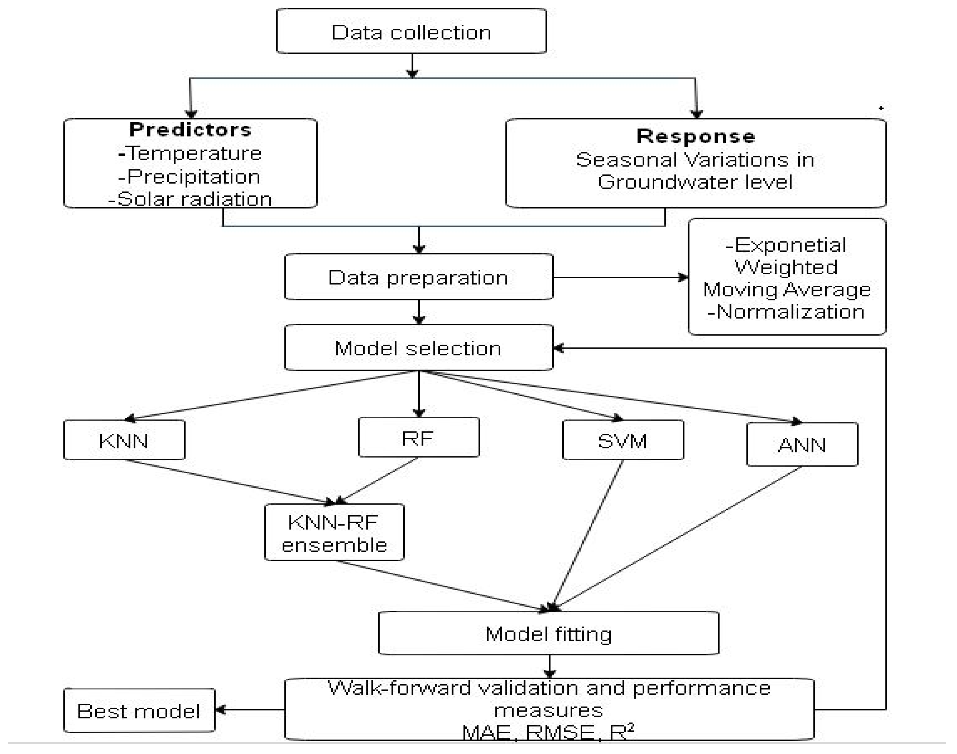
It is important that the prediction model is properly evaluated to assess its performance [87,88]. We estimated the predictive ability of the KNN-RF ensemble model on groundwater levels and evaluated it against SVM, KNN, RF, and ANN models based on mean absolute error (MAE), root mean square error (RMSE), the Nash–Sutcliffe efficiency coefficient (NSE), and the coefficient of determination ($R^2$). MAE, RMSE, and $R^2$ were selected because they limit the bias of models against acute events [88]. In addition, MAE and RMSE provide a finer comparison between models, especially in data-scarce situations [88]. NSE is another efficient coefficient used to gauge the relative magnitude of residual variance against the variance of observational data [46,88,89]. MAE, RMSE, and $R^2$ range between 0 and 1, while NSE is between −$\alpha$ and 1. The highest agreement between the estimated and observed values is reached when MAE = 0, RMSE = 0, NSE = 1, and $R^2$ =1. All measurements of the performance of the models were conducted using the hydrostats library (a Python package designed distinctively for hydrology studies) [90]. MAE, RMSE, NSE, and $R^2$ are defined as:

$$MAE=\frac{1}{n}{\displaystyle \sum _{i=1}^n\left|Q_i^E-Q_i^A\right|},$$

(4)

$$RMSE=\sqrt{{\displaystyle \sum _{i=1}^n{\left(Q_i^E-Q_i^A\right)}^2}},$$

(5)

$$R^2=\frac{{{\displaystyle {\sum }_{i=1}^n\left[\left(Q_i^E-{\overline{Q}}_i^E\right)\left(Q_i^A-{\overline{Q}}_i^A\right)\right]}}^2}{{\displaystyle {\sum }_{i=1}^n{\left(Q_i^E-{\overline{Q}}_i^E\right)}^2{\displaystyle {\sum }_{i=1}^n{\left(Q_i^A-{\overline{Q}}_i^A\right)}^2}}},$$

(6)

$$NSE=1-{\frac{{\displaystyle {\sum }_{i=1}^n\left[\left(Q_i^E-Q_i^A\right)\right]}}{{\displaystyle {\sum }_{i=1}^n{\left(Q_i^A-{\overline{Q}}_i^A\right)}^2}}}^2,$$

(7)

where $Q^E$ is the estimated change in groundwater level, $Q^A$ is the actual or observed groundwater level, and $n$ is the total number of input data points.

4. Methodology

The principal ambition of this study was to propose a decisive model to characterize the seasonal response of the fractured aquifer in eastern Rwanda, through quantification of seasonal deviations in water table depths in data-scarce situations. There is a requirement [19,24,26] for accessible and simple tools that offer actionable insights for the adaptive management of groundwater resources on a seasonal basis. With that requirement in mind, we propose to estimate seasonal groundwater levels using an innovative ensemble KNN-RF model with an exponentially weighted average preprocess of three predictors (solar radiation, precipitation, and temperature). The workflow of predictive modeling and validation setup is illustrated in Figure 6.

Figure 6. Flow chart of the KNN-RF method.

Potential features are selected from the collected data. Solar radiation, precipitation, temperature, and GWL data are refined and scaled for proper format and, subsequently, the candidate machine learning models are chosen. The two models (RF and KNN), both of which are non-complex and capable of working with both small and big datasets [66,70,91], are combined to overcome the disadvantages of small datasets as well as enhance predictive accuracy. In the final step, the models are tested and compared against NSE, MAE, RMSE, and $R^2$ using both estimated and observed groundwater data. A rolling window testing and validation method is employed and the most effective and useful model is determined based on the performance contrasts. This is most suited for the temporal nature of time series data [92], since the size of training and validation sets are sampled with respect to the desired forecast length (corresponding to 15, 30, 60, and 90 days) at the end of the series. A model that can be easily adopted using the available information, particularly in resource scarce areas, will be most feasible and practical for sensible decision making on groundwater resources.

4.1. K-Nearest Neighbor

K-Nearest Neighbor is a simple and robust method for regression and classification. Based on the proximity to the training data points, untrained data point(s) can be approximated utilizing the KNN method [91,93]. While attained observations are incomplete and noisy, the KNN technique is one of the best methods for ML-based forecasting [33,34]. Using this method, the most influential areas can also be identified from noisy samples. For continuous data, matching of points is done with respect to the distance measured using either Minkowski, Euclidean, Chebyshev, or Manhattan metrics. Suppose, there are two sets, $X$ and $Y$, and each of them has $t$ number of items, such that $X=\left(x_1,x_2,\dots ,x_t\right)$, and $Y=\left(y_1,y_2,\dots ,y_t\right)$ so long as ($j=1,2,3,\dots ,t$). Then the distance between the desired data point and the nearby points can be enumerated. The distance between the desired point to the closest points is then defined as:

$$\widehat{D}\left(X,Y\right)={{\displaystyle \sum _{j=1}^t\left[\left({\left|x_j-y_j\right|}^r\right)\right]}}^{1/r}$$

(8)

where $r$ is a positive real number, and $\widehat{D}$ is the calculated distance.

• To anticipate the target value, we perform the following steps:
• Use Equation (8) to calculate the distance between a new sample and each of the adjacent points.
• Sort all values calculated in step 1 by increasing order.
• Utilize the greedy search technique to determine the optimal value of K, based on RMSE.
• Enumerate an inverse distance weighted mean using K neighboring examples.
• Return average as the approximated value.

In the above scheme, K is a user-configurable parameter that represents the number of contiguous features to be included in the calculation of average votes. The prediction of variations in groundwater levels is obtained as the average weighted distance between samples.

4.2. Artificial Neural Network

The artificial neural network is a combination of multiple interconnected neurons that learn cardinal relationships in a set of data in the same way as the human brain operates [37,94,95]. Interconnected neurons make an input layer, one or more hidden layers, and an output layer. As input data are fed through the input layer, neurons in the hidden layer(s) compute the output using connection weights and bias. One of the two stages in which ANNs are used is in the training phase. In this phase, a training algorithm such as conjugate gradient momentum, Levenberg–Marqardt, backpropagation, Adam, gradient-descent, or Bayesian regularization is selected and the suitable connection weights are determined. The feed-forward network was trained using the back-propagation method to avoid an over-fitting issue. Another stage is the real application of the trained neural network. The estimated value(s) is then obtained as:

$$Y_e=f{\displaystyle \sum _{j=1}^k\left(x_i{w}_{ij}+b\right)}$$

(9)

where $x_i$ is the input examples, $Y_e$ is the approximated output, $b$ is bias term, $f$ is an activation function, and $w_i$ is the weight of the vertices. In a three-layered multilayer perceptron network, the transformation of the weighted inputs is accomplished using a rectifier linear unit (ReLU), which is defined as:

$$x_r=\max \left(0,x_i\right)$$

(10)

where $x_r$ symbolizes the transformed input passing in the hidden layer, and $x_i$ is the raw input. All $x_i$ values greater than zero are mapped to their respective y-values, while all $x_i$ values less than zero are assigned to zero. This makes the ReLU computational modest and able to efficiently handle negative inputs, and also offers smoother optimization [96].

4.3. Support Vector Machine

The support vector machine for regression problems is termed as a support vector regression (SVR). SVRs are supervised learning techniques introduced by Cortes and Vapnik [97]. These are powerful methods that utilize structural risk minimization to obtain optimal solutions [97,98]. SVR accomplishes risk minimization measures using a set of several input vectors while conducting an estimation of non-linear targets through regression processes [98,99]. Based on the assumption that, there is a relationship between the dependent variable $y$ and independent variables $\left(X_1,X_2,X_3,\dots ,X_t\right)$, the SVR model estimates a function $f\left(x\right),$ which determines the target values $y_i$ plus the admissible error $ϵ$. In an SVR model, data processing is conducted in a hyperplane and it starts as a linear transformation of the time-series. The linear representation of an SVR algebraic function is given by:

$$F=⟨w,x⟩+b,$$

(11)

$$Y=f\left(x\right)+ϵ,$$

(12)

where $bϵR$, $x$, $wϵx$, and $⟨w.x⟩$ are the bias, inputs signals, weight vector, and the dot product between $x$ and $w,$ respectively. Then to minimize the norm $\parallel w{\parallel }^2=⟨w.x⟩,$ we need to find the smallest possible value of $w$ as:

$$minimize\frac{1}{2}\parallel w{\parallel }^2,$$

(13)

subject to:

$$⟨w,x⟩+b-Y_i\le ϵ;Y_i-⟨w,x⟩-b\le ϵ;ϵ\ge 0;i=1,2,\dots ,t.$$

(14)

As the primary goal is to get a function f(x) that can be used to calculate a set of the observed $x_i$ and the estimated $y_i$ values with the level of accuracy bounded by $ϵ,$ this is realized by minimizing a regularized risk function in $(\mathrm{Equation} (13$)$)$ with constraints stipulated in inequalities given below (Equation (14)). Two relaxed variables ($\xi$, ${\xi }^{*}$) are incorporated in (Equation (15)) to allow for some error tolerance.

$$\frac{1}{2}{‖w‖}^2+C\left({\displaystyle \sum _{i=1}^t\left(\xi +{\xi }^{*}\right)}\right)$$

(15)

subject to:

$$⟨w,x⟩+b-Y_i\le ϵ+{\xi }^{*};Y_i-⟨w,x⟩-b\le ϵ+\xi ;{\xi }^{*}+\xi \ge 0;i=1,2,\dots ,t$$

(16)

where $t$ is the total number of model input features, and C is a user-configurable parameter that manages the influence of each supporting vector in the generalization and stability of the SVR model. Ultimately, Equation (12) can be reformulated as:

$$F\left(x,{\alpha }_i,{\alpha }_i{}^{*}\right)={\displaystyle \sum _{i=1}^t\left({\alpha }_i-{\alpha }_i{}^{*}\right)}k⟨x,x_i⟩+b$$

(17)

where $k⟨x,x_i⟩$ is the kernel, and ${\alpha }_i,{\alpha }_i{}^{*}$ are Lagrangian multipliers. Before applying SVR in data processing, the appropriate kernel and support vectors should be determined. The SVR kernel provides mapping of the non-linear features in a high dimensional space while converting it into a normal linear format. Thus, SVR suits well for complex interrelationship among features in environmental modeling [59]. There are several types of kernels, such as polynomial, multi-layer perceptron, exponential, and Gaussian radial basis function. Radial basis essence has shown a commended performance in hydrologic studies [99,100]. The exponential radial bias function is given by:

$$k\left(x_i,x\right)=\exp \left(-\parallel \left(x_i-x_t\right){\parallel }^2\right)÷2{\sigma }^2.$$

(18)

4.4. Random Forest

Based on decision trees with the application of bootstrap aggregation, random forests (RF) for regression problems and classification were introduced by Breiman [101]. A forest of diverse trees is developed using randomly chosen features selected from random subsets of the original training data. As a large number of trees is produced, classification results are obtained from the popular class, while in regression problems, the result is computed as the average value obtained from all the individual regression trees [102,103]. In the current study, we focus on the regression type of RF. A forest may contain several trees as specified by the user. Suppose the number of trees in the forest is denoted by $M$. The random forest method works in the following manner:

• Randomly fetch different subsets $x_i$ from a given dataset $X$.
• Use sampled data to create $M$ decision trees.
• Enumerate average of the votes from the decision trees.
• Return the average as the final approximated value.

Randomness is applied at two levels of the random forests: during data selection and in attribute selection. Since the regression trees are created from random vectors selected from training dataset $X$, each leaf-node contains a constant estimate of $Y$. As an example, the data points $\left\{\left(x_1,y_1\right),\left(x_2,y_2\right),\dots ,\left(x_M,y_M\right)\right\}$ are selected as samples for the leaf-nodes, and the anticipated data can be modeled as the averaged predictions from all the individual regression trees as:

$$\widehat{y}\left(x_j\right)=\frac{1}{M}{\displaystyle \sum _{m=1}^M{y}_m\left(x_j\right)},$$

(19)

such that $j=1,2,\dots ,M$, and where $\widehat{y}\left(x_j\right)$ is the estimated result. In RF, tuning-parameters have a great effect on the ability of the model [78]. The most important tuning parameters for RF in Scikit-Learn are n_estimators, random_state, n_jobs, min_sample_leaf, and max_features [78].

4.5. KNN-RF Ensemble

Focusing on the improvement of seasonal predictions, a hybrid KNN-RF technique is developed and validated. As indicated in the Introduction section, the RF and KNN methods have good data-representation ability; however, these methods do not perform optimally when fed with tiny datasets. To overcome this limitation, we merge the above models in a hybrid manner. The two base regressors, KNN, and RF are fitted on the whole training set and, using the test set, the models yield predictions individually. The results are then averaged to produce the final result. The final result of the KNN-RF ensemble is given by:

$$\mu (x)=\frac{1}{N}{\displaystyle \sum _{n=1}^N{\omega }_n{p}_n}(x)$$

(20)

where $\mu \left(x\right)$ is the final weighted average result of the ensemble model, ${\omega }_n$ is the weight allocated to the $n^{th}$ regressor, which is based on the $MSE$ performance; $p_n$ is the prediction from $n^{th}$ model; $x$ is the sample data points. The ensemble based on the KNN-RF method enhances predictive performance in the following aspects [104].

• Supports using fewer samples to adequately represent data distribution.
• Limits the generalization error.
• Controls variance in a small dataset.
• Relieves the processing burden for model selection.

Uniform weights are assigned to all estimators in the KNN-RF model. The base RF model is set to perform bootstrapping on the training subset, which reduces similarities in the trees. This, therefore, benefits the performance of the model provided that a small number of training examples are accessible. The KNN base model is set to use the distance between data points as the proximity criterion. Tuning parameters for KNN-RF are leaf_size, metric, random_ state, n_jobs, n_neighbors, $p$, and weights.

4.6. Tuning Parameter and Input Selection

Based on the performance gains of the models, the appropriate tuning parameters are selected to establish the proper architecture for each of the model during the training phase. Each input arrangement was assessed for the following parameters in Scikit-Learn. For KNN, the Chebyshev, Minkowski, Euclidean, and Manhattan length metrics were tested. The Minkowski measure emerged as the best choice. [105]. The ideal value of K was found using a grid-search procedure [106], and it varied with the sample size, which was determined by the prediction range (more details about the portions of the sample used for the adjustments and testing of the models are given in the next subsection). For ANN, the trial-and-error technique was used to determine the finest number of hidden layer neurons based on the least RMSE [53,107,108]. Fourteen hidden neurons produce the best output. The adaptive learning (Adam) optimization scheme was found to be the most suitable for the dataset used in the current investigation [109]. The ReLU, linear, and tanh activation functions were tested and resulted in ReLU enumerating the most precise results [96,110].

Considering the SVR, the most appropriate values of the epsilon, cost, gamma, and the kernel (rbf, poly, sigmoid) were verified using the trial-and-error technique [53] producing the best factors of 0.01, 1.0, scale, and RBF, respectively [111]. For RF and KNN-RF, the ideal number of estimators is enumerated using the grid search procedure [112]. The number of learners affects the processing speed of the model. Whilst a large number of learners improves the reliability of the model, it also slows down processing speed [78]. The ideal number of estimators is 200, max_depth of the trees is 15, leaf_size is 30, max_feature is n _feature, min_sample_leaf is 1, random_state is none, n_jobs is 1, and min_split is 2. Similarly, the n_neighbors is 3 when the prediction period is 15 or 30 days, and 2 when the prediction period is 60 or 90 days, $p$ is 2, metric is Minkowski, random _ state is 0, and weights is distance.

For proper and comparable evaluation of the models, the input series of the time lagged precipitation, groundwater level, temperature, and solar radiation were arranged in twelve combinations: P (t − 1) L (t) T (t) S (t), P (t − 2) L (t) T (t) S (t), P (t − 3) L (t) T (t) S (t), P (t − 4) L (t) T (t) S (t), P (t) L (t) T (t) S (t − 1), P (t) L (t) T (t) S (t − 2), P (t) L (t) T (t) S (t − 3), P (t) L (t) T (t) S (t − 4), P (t) L (t) T (t − 1) S (t), P (t) L (t) T (t − 2) S (t), P (t) L (t) T (t − 3) S (t), and P (t) L (t) T (t − 4) S (t). Once the best parameters and input arrangements were established, the KNN − RF, SVM, ANN, RF, and KNN models were trained as described in the next subsection.

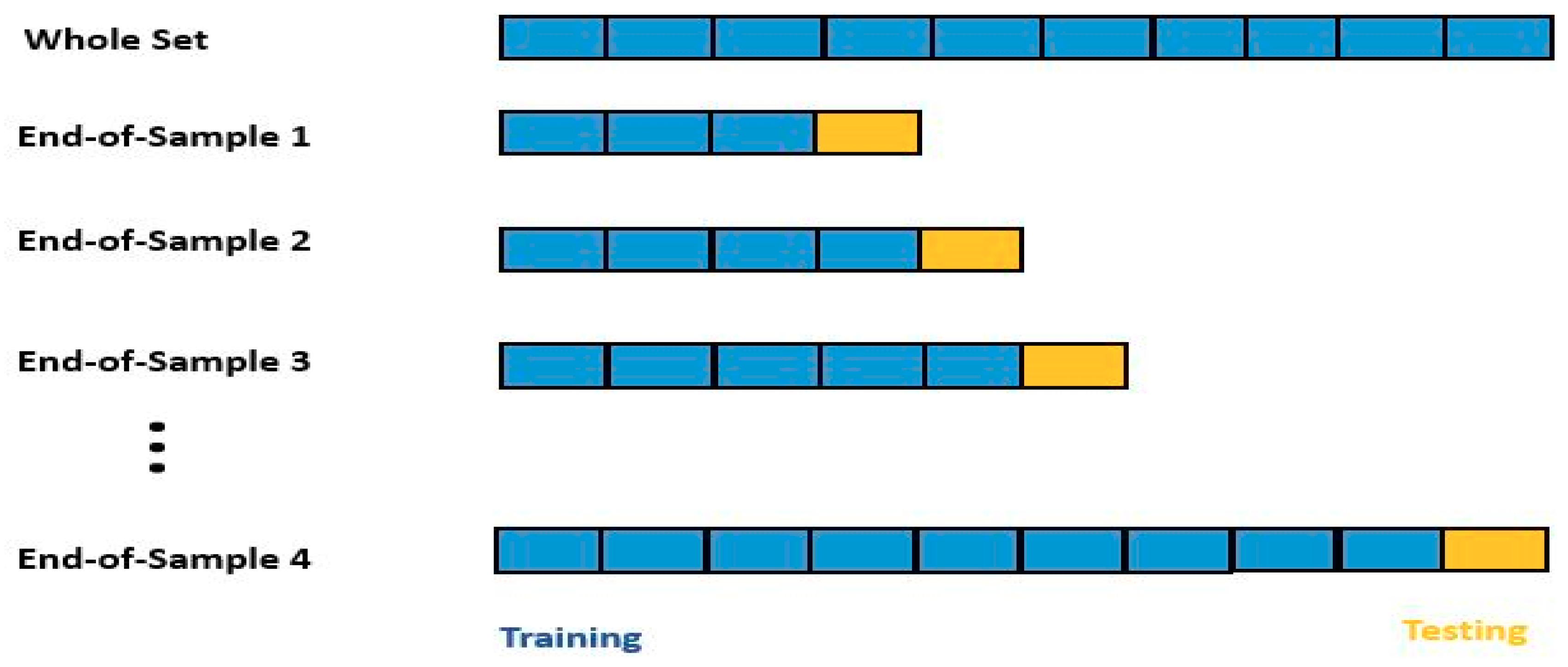
4.7. Training and Testing of the Model

When it comes to the training and evaluation of the models, time series predictive modeling has numerous distinctive traits and peculiarities that need a different approach to supervised learning problems [92]. There are intrinsic interrelationships between the data points measured across time, and during the training and testing of the models, the temporal structure of the series needs to be maintained. Typically, the arbitrary splitting of the timeseries dataset from different points in time is irrelevant to time-based data because it causes inherent biases [92]. The rolling window or walk-forward validation is best suited for time series-based forecasting as it facilitates updating of the predictions as new data come in. In this approach, the holdout values are sampled at the end of the dataset temporally. Figure 7 shows a graphic demonstration of the rolling windows validation procedure.

Figure 7. Diagram of the time series 4-sliding window validation method. Adapted from LaBarr (2018).

The size of the holdout sample is determined by the prediction scope and, therefore, the width of the rolling window is equal to the desired forecast length. The training and validation of the KNN-RF, ANN, SVM, RF, and KNN models was conducted with the rolling window technique. It was completed using four different portions of training and holdout values corresponding to the prediction of 15-day-ahead (t + 15), 30-day-ahead (t + 30), 60-day-ahead (t + 60), and 90-day-ahead (t + 90). The training and validation percentages for these prediction horizons were $88.1423-11.8577$, $92.0949-7.9051$, $96.0473-3.9527$, and $98.0237-1.9763$, respectively. The trained models that were used for prediction are explained in the next subsection.

4.8. Prediction of Seasonal Changes in Groundwater Depths

In this work, seasonal forecasting is the forecast of 90 days lead-time groundwater level variations. For comparison, other prediction periods of 15, 30, and 60-day were also evaluated. As previously explained, the 15, 30, 60, and 90 days predictions were implemented by changing the size of the hold-out sample.

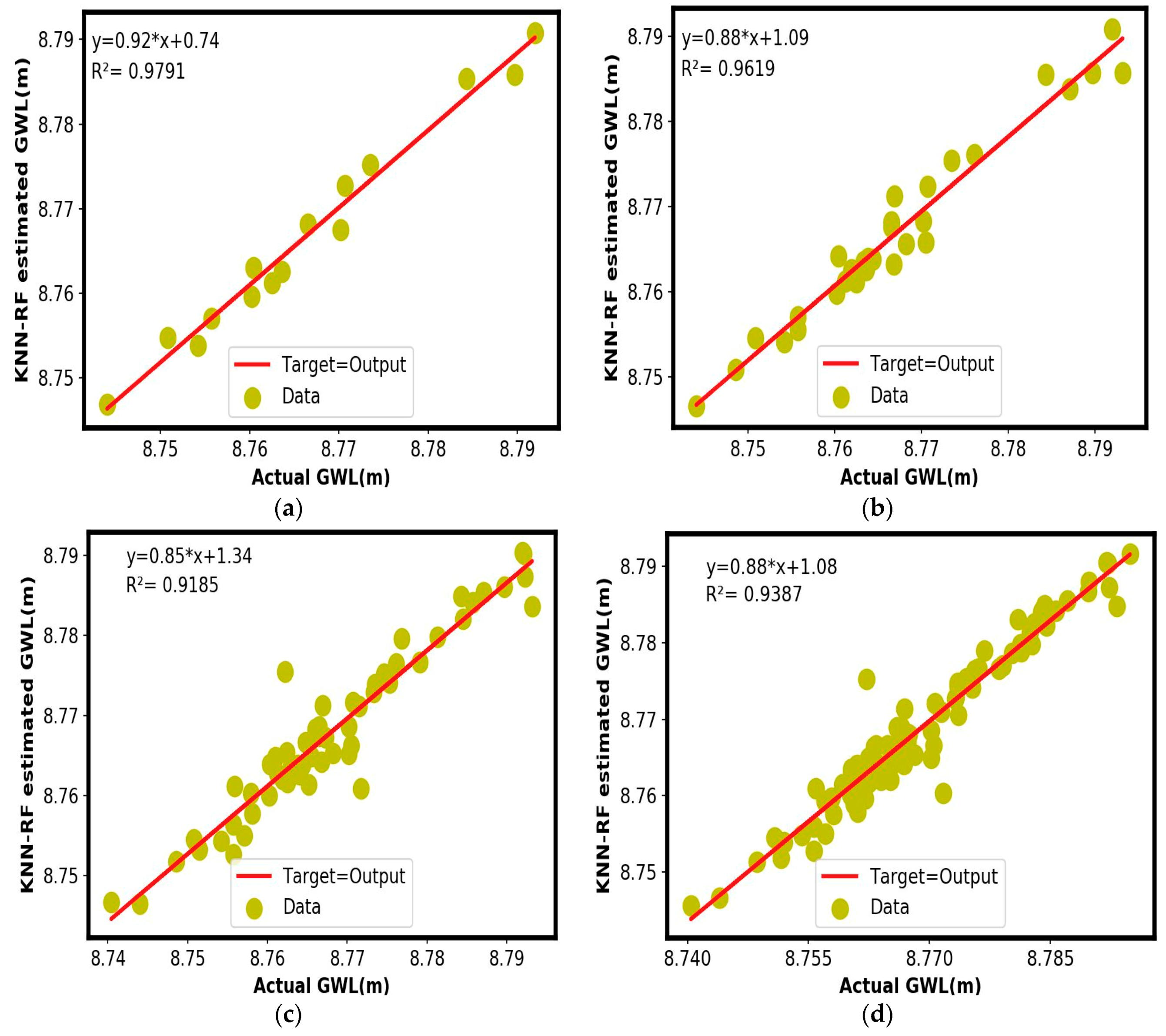
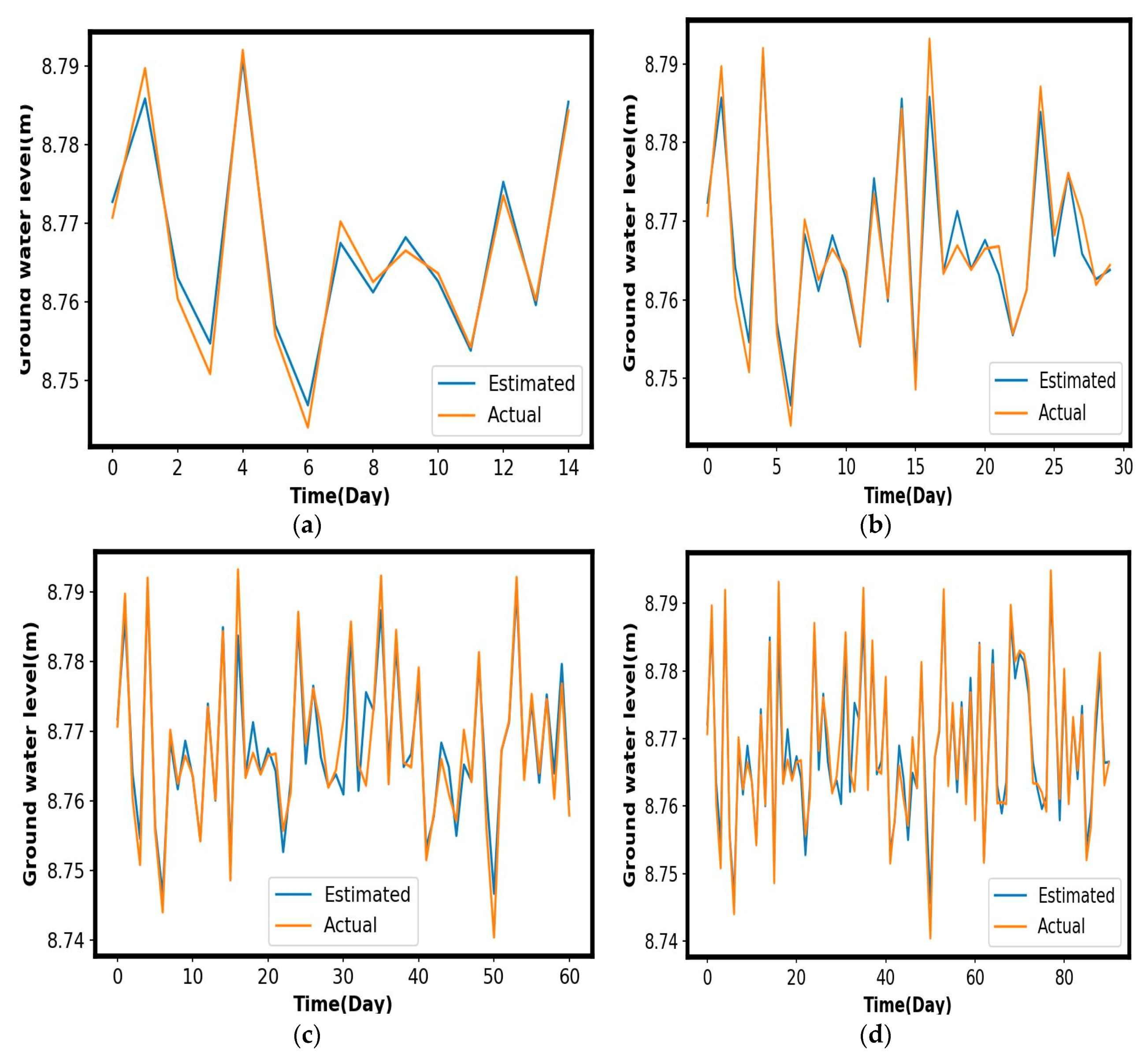
5. Experimental Results and Discussion

The predictive capacity of the KNN-RF technique was investigated and the results were compared to the four general models. The results of the 15, 30, 60, and 90 days lead-time groundwater level predictions at the Mukarange borehole using the KNN-RF, RF, SVM, ANN, and KNN models are presented in Figure 8. According to Figure 8, at all horizons the KNN-RF model achieved the best performance with respect to $\mathrm{NSE},\mathrm{MAE},\mathrm{RMSE}$ and $R^2$ values. For this model, the $\mathrm{RMSE}$ values range between $0.0030$ and $0.0035,$ while $\mathrm{NSE}$ values were between $0.913$ and $0.9741$ during the validation stage. The KNN model obtained the best results for the short term (15–30 day-ahead), while RF obtained improved accuracy for long-range (60–90 day-ahead) estimations. The SVR model tried to catch up with the long changes of the levels and outperformed the ANN model. Similar findings were reported in the studies that compared the above methods for the modeling of groundwater tables [50,113,114]. At all lead times, the ANN method overpredicted the observed values. The low performance of the ANN method in training and testing phases on small-sized samples could be attributed to the data requirements of this model [115]. Compared with the RF, ANN, and SVM models, the KNN model had higher performance scores. This is in contrast with the outcomes reported by Rahmati et al. [116]. Meanwhile, RF is found to be superior to the SVM model, which is consistent with the conclusion made by Naghibi et al. [117].

Figure 8. Comparison of the performance obtained by the SVR, ANN, RF, KNN, and KNN-RF models for 15, 30, 60, and 90 day-ahead groundwater level prediction.

From Table 2 and Table 3, the highest accuracy of the KNN-RF for different horizons was achieved with precipitation (P−1), solar radiation S(t), temperature T(t), and groundwater level L(t) time-lags in the testing phase. The most accurate outcomes are shown for the prediction at 15-days ahead. It is also seen that the accuracy of the forecasted results declines with the length of the prediction. These results are in corroboration with the studies in [58,60]. Conversely, the 90-day prediction obtained better results than 60-day prediction. The largest difference between the MAE and RMSE values is perceived for the 60-day predictions. The $R^2$ criterion values showed higher importance for longer lead-times, while $\mathrm{NSE}$ provided the overall description of the predictive power of the models.

Table 2. Performance evaluation criteria for 15, 30 60, and 90 days lead-time groundwater level variations using the KNN-RF model.

	L (t + 15)			L (t + 30)			L (t + 60)			L (t + 90)
Input Arrangement	RMSE	MAE	${\mathit{R}}^2$	RMSE	MAE	${\mathit{R}}^2$	RMSE	MAE	${\mathit{R}}^2$	RMSE	MAE	${\mathit{R}}^2$
P (t−1) S (t) T (t)	0.0022	0.0019	0.9791	0.0026	0.0020	0.9619	0.0036	0.0025	0.9185	0.0031	0.0022	0.9387
P (t−2) S (t) T (t)	0.0061	0.0050	0.8397	0.0069	0.0050	0.7114	0.0068	0.0051	0.7049	0.0065	0.0048	0.7143
P (t−3) S (t) T (t)	0.0054	0.0043	0.8909	0.0064	0.0047	0.7527	0.0059	0.0044	0.7948	0.0059	0.0044	0.7807
P (t−4) S (t) T (t)	0.0049	0.0042	0.9179	0.0069	0.0051	0.7739	0.0056	0.0042	0.7989	0.0057	0.0043	0.7882
P (t) S (t−1) T (t)	0.0060	0.0051	0.8401	0.0067	0.0051	0.7308	0.0064	0.0048	0.7454	0.0061	0.0046	0.7660
P (t) S (t−2) T (t)	0.0060	0.0051	0.8749	0.0061	0.0048	0.7872	0.0059	0.0047	0.7993	0.0061	0.0046	0.7706
P (t) S (t−3) T (t)	0.0058	0.0048	0.8639	0.0065	0.0048	0.7438	0.0059	0.0044	0.7948	0.0059	0.0044	0.7783
P (t) S (t−4) T (t)	0.0058	0.0050	0.8635	0.0062	0.0049	0.7739	0.0061	0.0049	0.7537	0.0057	0.0044	0.7840
P (t) S (t) T (t−1)	0.0061	0.0050	0.8391	0.0065	0.0049	0.7577	0.0065	0.0049	0.7408	0.0065	0.0048	0.7277
P (t) S (t) T (t−2)	0.0061	0.0050	0.8411	0.0065	0.0049	0.7601	0.0065	0.0049	0.7518	0.0062	0.0046	0.7553
P (t) S (t) T (t−3)	0.0058	0.0048	0.8539	0.0064	0.0048	0.7545	0.0062	0.0048	0.7646	0.0059	0.0046	0.7711
P (t) S (t) T (t−4)	0.0057	0.0047	0.8663	0.0066	0.0049	0.7312	0.0062	0.0048	0.7578	0.0059	0.0045	0.7679

T represents temperature, L represents groundwater level, S represents solar radiation, and P represents precipitation. The highest $R^2$ and lowest MAE and RMSE are in bold.

Table 3. NSE performance evaluation criteria for 15, 30 60, and 90 day-ahead groundwater level predictions using the KNN-RF model.

	L (t + 15)	L (t + 30)	L (t + 60)	L (t + 90)
Input Arrangement
P (t−1) S (t) T (t)	0.9741	0.9540	0.9130	0.9346
P (t−2) S (t) T (t)	0.7957	0.6792	0.6657	0.6898
P (t−3) S (t) T (t)	0.8385	0.7239	0.7532	0.7483
P (t−4) S (t) T (t)	0.8697	0.6798	0.7720	0.7595
P (t) S (t−1) T (t)	0.7987	0.6977	0.7083	0.7267
P (t) S (t−2) T (t)	0.8014	0.7458	0.7488	0.7290
P (t) S (t−3) T (t)	0.8105	0.7136	0.7532	0.7431
P (t) S (t−4) T (t)	0.8160	0.7373	0.7339	0.7659
P (t) S (t) T (t−1)	0.7934	0.7168	0.6968	0.6951
P (t) S (t) T (t−2)	0.7933	0.7173	0.7023	0.7212
P (t) S (t) T (t−3)	0.8133	0.7256	0.7274	0.7456
P (t) S (t) T (t−4)	0.8214	0.7055	0.7260	0.7430

T represents temperature, L represents groundwater level, S represents solar radiation, and P represents precipitation. The highest $NSE$ are in bold.

Figure 9 delineates the results of the comparison of the relationships between the actual and KNN-RF estimated groundwater levels for different horizons. These results show that there is high association between the actual and estimated levels for all four-time horizons. The 15-day range exhibits the largest value of $R^2$, since most of the predictions are closer to the straight line. It was also found that the 60-day prediction range showed the relatively lowest value of $R^2$ compared to other ranges. This also supports the results presented in Figure 8, which showed higher error values for the 60-day prediction stage than those of the other predictions. Similarly, the hydrographs in Figure 10 show that the KNN-RF technique reproduced and fairly represented the seasonal oscillations of the depths of the groundwater tables. However, it is quite obvious that the 60-day prediction is not as accurate as the predictions for other time-horizons.

Figure 9. Assessment of the actual and the estimated groundwater levels of the optimal KNN-RF model for 15, 30, 60, and 90 days (corresponding to a–d, respectively) lead time in the testing phase.

Figure 10. Comparison of the 15, 30, 60, and 90 days (corresponding to a–d, respectively) estimated and the actual levels yielded by the optimal KNN-RF technique.

The results obtained have also demonstrated the significant role of input and tuning parameter selection. The combinations of solar radiation, temperature, precipitation, and previous groundwater level with an appropriate time-lag improved the seasonal estimation of the groundwater heights. It was found that for the KNN-RF technique, the lagged precipitation improved $\mathrm{NSE},\mathrm{MAE},\mathrm{RMSE}$, and $R^2$ scores, for 32.6%, 53.19%, 51.57%, and 27.38%, respectively. This suggests that there is a huge potential for the infiltrated and percolated rain water to raise the groundwater table for the Mukarange aquifer.

For feature selection, Lindsey et al. [82] and Kelly et al. [83] showed that the use of solar radiation as a substitute for evapotranspiration as a suitable option for capturing the dynamics of groundwater depth. Our results confirmed the high influence of solar radiation on the long-term variability of groundwater levels in the semi-arid area.

Results also confirmed that tuning parameters have a great influence on the model’s final results. These parameters led to an improved generalization capability for all models. Considering the SVR, it was found that RBF yielded the best performance, while epsilon and gamma are the most influential parameters for the determination of the appropriate architecture of the SVR model. This is in corroboration with the findings in [59]. With six (6) input features, the finest number of nodes in the hidden layer of the ANN was found to be 14, which is consistent with the conclusion reached by Kayzoglu et al. [118]. Whilst the adaptive learning scheme and the ReLU function are commonly used with large datasets, our results suggest that these parameters can also work well with a limited dataset. One of the possible reasons for this outcome is the sparsity of the available samples. We found that limiting the number of learners to 200 and the depth of the trees to 15 had positive effects on the generalization ability of the RF model and overcame the overfitting issue on the Mukarange dataset. The best results for the KNN-RF, SVM, and ANN methods were achieved with the structures presented in Table 4.

Table 4. Summary of the selected parameters during training of the SVR, ANN, and KNN-RF models.

SVR	ANN	KNN-RF
Epsilon: 0.01	Epsilon: 0.0001	Epsilon: 0.01
Kernel: RBF	Hidden layer: 1	Number of trees: 200
Gamma: Scale	Hidden layer neurons: 14	Maximum depth: 15
Soft-margin(C): 1.0	Activation function: ReLU	Weights: distance
Support vectors: 137	Learning mode: Adaptive	Metric: Minkowski
Degree: 3	Max-iterations: 500	Number of estimators: 50
	Training algorithm: Adam	Algorithm: Auto

In general, the KNN-RF model has experimentally demonstrated its superiority to classical models. For example, despite the sparseness of the available dataset, multi-step prediction results obtained by the KNN-RF model outperformed SVR, KNN, RF, and ANN scores. The researchers recognize some limitations to the approach applied in this study as, for example, the size of the dataset might not properly represent the distribution of climatic and groundwater data.

6. Conclusions

The performance and capacity of the ensemble KNN-RF regression approach to the prediction of seasonal groundwater levels for the fractured aquifer with limited data has been examined in this study. Groundwater level data and its significant meteorological drivers (solar radiation, temperature, and precipitation) collected from Mukarange in eastern Rwanda were used for the analysis. From the experimental analysis, it was found that the KNN-RF ensemble approach is stable with enhanced generalization competence and prediction accuracy. The results also indicated that, by using the sliding window validation procedure, the KNN-RF model captured slightly well with the time-based changes in the depths of the groundwater tables. Inclusion of the solar radiation as a substitute for evapotranspiration resulted in an improved prediction accuracy. The results of the study suggest that KNN-RF is well-suited for the forecasting of seasonal variations in groundwater depths with limited samples. The values of the analytical measures showed that, in all prediction ranges, the KNN-RF technique achieved the most promising results compared to those obtained by the ANN, KNN, SVM, and RF models. The $\mathrm{NSE}$ and $R^2$ values of the ensemble KNN-RF technique were higher than those yielded by the above methods, and the values of $\mathrm{RMSE}$ and $\mathrm{MAE}$ of the ensemble KNN-RF were smaller than those produced by the other methods. The research used data from one groundwater observation station over a short duration, and it has been concluded that more data could improve the predictive accuracy of the model. This can be achieved simply and effectively by updating the model as data become available, since a sliding window method has been used. In addition, the KNN-RF model was shown to be an advanced alternative to the SVR, KNN, RF, and ANN models. The results from this study would be useful for the planning and management of groundwater resources. Our proposed model could be readily transferable or adapted to other areas, specifically those with similar aquifers where the availability and quantity of data is challenging. In order to address data scarcity issues, the authors intend to establish a low-cost, low power wireless sensor network for near real-time monitoring of groundwater levels in eastern Rwanda.

References

- Robins, N.S.; Fergusson, J. Groundwater scarcity and conflict–managing hotspots. Earth Perspect. 2014, 1, 6. [Google Scholar] [CrossRef]
- Khosravi, K.; Pham, B.T.; Chapi, K.; Shirzadi, A.; Dou, J.; Revhaug, I.; Prakash, I.; Bui, D.T. A comparative assessment of decision trees algorithms for flash flood susceptibility modeling at Haraz watershed, northern Iran. Sci. Total. Environ. 2018, 627, 744–755. [Google Scholar] [CrossRef] [PubMed]
- Rulli, M.C.; D’Odorico, P. The water footprint of land grabbing. Geophys. Res. Lett. 2013, 40, 6130–6135. [Google Scholar] [CrossRef]
- Macdonald, A.; Bonsor, H.C.; Dochartaigh, B.É.Ó.; Taylor, R.G. Quantitative maps of groundwater resources in Africa. Environ. Res. Lett. 2012, 7, 024009. [Google Scholar] [CrossRef]
- Döll, P.; Hoffmann-Dobrev, H.; Portmann, F.; Siebert, S.; Eicker, A.; Rodell, M.; Strassberg, G.; Scanlon, B.R. Impact of water withdrawals from groundwater and surface water on continental water storage variations. J. Geodyn. 2012, 59, 143–156. [Google Scholar] [CrossRef]
- Healy, R.W. The future of groundwater in sub-Saharan Africa. Nature 2019, 572, 185–187. [Google Scholar] [CrossRef]
- Castellazzi, P.; Martel, R.; Galloway, D.L.; Longuevergne, L.; Rivera, A. Assessing groundwater depletion and dynamics using GRACE and InSAR: Potential and limitations. Ground Water 2016, 54, 768–780. [Google Scholar] [CrossRef]
- Macdonald, A.; Bonsor, H.C.; Ahmed, K.M.; Burgess, W.; Basharat, M.; Calow, R.C.; Dixit, A.; Foster, S.S.D.; Gopal, K.; Lapworth, D.J.; et al. Groundwater quality and depletion in the Indo-Gangetic Basin mapped from in situ observations. Nat. Geosci. 2016, 9, 762–766. [Google Scholar] [CrossRef]
- Richey, A.S.; Thomas, B.; Lo, M.-H.; Reager, J.T.; Famiglietti, J.; Voss, K.; Swenson, S.; Rodell, M. Quantifying renewable groundwater stress with GRACE. Water Resour. Res. 2015, 51, 5217–5238. [Google Scholar] [CrossRef] [PubMed]
- Makoto, T. Groundwater as a Key of Adaptation to Climate Change. In Groundwater as a Key for Adaptation to Changing Climate and Society; Springer: Tokyo, Japan, 2014; Volume 6, pp. 17–27. [Google Scholar]
- Water, U.N. Wastewater Management—A UN-Water Analytical Brief; UN Water: New York, NY, USA, 2015. [Google Scholar]
- Hass, J.C.; Birk, S. Characterizing the spatiotemporal variability of groundwater levels of alluvial aquifers in different settings using drought indices. Hydrol. Earth Syst. Sci. 2017, 21, 2421–2448. [Google Scholar] [CrossRef]
- De Graaf, I.; Van Beek, R.L.; Gleeson, T.; Moosdorf, N.; Schmitz, O.; Sutanudjaja, E.H.; Bierkens, M.F.P. A global-scale two-layer transient groundwater model: Development and application to groundwater depletion. Adv. Water Resour. 2017, 102, 53–67. [Google Scholar] [CrossRef]
- Rathay, S.; Allen, D.; Kirste, D. Response of a fractured bedrock aquifer to recharge from heavy rainfall events. J. Hydrol. 2018, 561, 1048–1062. [Google Scholar] [CrossRef]
- Stoll, S.; Franssen, H.H.; Butts, M.; Kinzelbach, W. Analysis of the impact of climate change on groundwater related hydrological fluxes: A multimodel approach including different downscaling methods. Hydrol. Earth Syst. Sci. 2011, 15, 21–38. [Google Scholar] [CrossRef]
- Cuthbert, M.O.; Tindimugaya, C. The importance of preferential flow in controlling groundwater recharge in tropical Africa and implications for modelling the impact of climate change on groundwater resources. J. Water Clim. Chang. 2010, 1, 234–245. [Google Scholar] [CrossRef]
- Yu, H.; Feng, Q. Comparative study of hybrid-wavelet artificial intelligence models for monthly groundwater depth forecasting in extreme arid regions, Northwest China. Water Resour. Manag. 2018, 32, 301–323. [Google Scholar] [CrossRef]
- Uhlemann, S.; Smith, A.; Chambers, J.; Dixon, N.; Dijkstra, T.; Haslam, E.; Meldrum, P.; Merritt, A.; Gunn, D.; Mackay, J. Assessment of ground-based monitoring techniques applied to landslide investigations. Geomorphol. 2016, 253, 438–451. [Google Scholar] [CrossRef]
- Yang, W. The Hydroclimate of East Africa: Seasonal Cycle, Decadal Variability, and Human-Induced Climate Change. Ph.D. Thesis, Columbia University, New York, NY, USA, 2015. [Google Scholar]
- Hyland, M.; Russ, J. Water as destiny- The long-term impacts of drought in sub-Saharan Africa. World Dev. 2019, 115, 30–45. [Google Scholar] [CrossRef]
- Xu, Y.; Seward, P.; Gaye, C.; Lin, L.; Olago, D.O. Preface: Groundwater in sub-Saharan Africa. Hydrogeol. J. 2019, 27, 815–822. [Google Scholar] [CrossRef]
- Van Engelenburg, J.; Hueting, R.; Rijpkema, S.; Teuling, A.J.; Uijlenhoet, R.; Ludwig, F. Impact of changes in groundwater extractions and climate change on groundwater-dependent ecosystems in a complex hydrogeological setting. Water Resour. Manag. 2018, 32, 259–272. [Google Scholar] [CrossRef]
- Matengu, B.; Xu, Y.; Tordiffe, E. Hydrogeological characteristics of the Omaruru Delta Aquifer System in Namibia. Hydrogeol. J. 2019, 27, 857–883. [Google Scholar] [CrossRef]
- Aboniyo, J.; Umulisa, D.; Bizimana, A.; Kwisanga, J.M.P.; Mourad, K.A. National Water Resources Management Authority for a Sustainable Water Use in Rwanda. Sustain. Resour. Manag. J. 2017, 2, 1–15. [Google Scholar]
- Abimbola, O.; Wenninger, J.; Venneker, R.; Mittelstet, A. The assessment of water resources in ungauged catchments in Rwanda. J. Hydrol. Reg. Stud. 2017, 13, 274–289. [Google Scholar] [CrossRef]
- Report Strategic Programme for Climate Resilience. 2017. Available online: https://www.climateinvestmentfunds.org/sites/cif_enc/files/knowledge-documents/rwanda_spcr_2017pdf.pdf (accessed on 26 October 2019).
- Ministry of Natural Resources. Water Resources Management Sub-Sector Strategic Plan (2011–2015). 2011. Available online: http://minirena.gov.rw/fileadmin/Land_Subsector/Water/Rwanda-Waterstrategy-04062011-final-1006-corrected1406_01.pdf (accessed on 26 October 2019).
- Gong, H.; Pan, Y.; Zheng, L.; Li, X.; Zhu, L.; Zhang, C.; Huang, Z.; Li, Z.; Wang, H.; Zhou, C. Long-term groundwater storage changes and land subsidence development in the North China Plain (1971–2015). Hydrogeol. J. 2018, 26, 1417–1427. [Google Scholar] [CrossRef]
- Tang, Q.; Oki, T. (Eds.) Terrestrial Water Cycle and Climate Change: Natural and Human-Induced Impacts; John Wiley & Sons: Hoboken, NJ, USA, 2016; Volume 221. [Google Scholar]
- Kenda, K.; Čerin, M.; Bogataj, M.; Senožetnik, M.; Klemen, K.; Pergar, P.; Laspidou, C.; Mladenic, D. Groundwater Modeling with Machine Learning Techniques: Ljubljana polje Aquifer. Multidiscip. Digit. Publ. Inst. Proc. 2018, 2, 697. [Google Scholar] [CrossRef]
- Shortridge, J.E.; Guikema, S.D.; Zaitchik, B.F. Machine learning methods for empirical streamflow simulation: A comparison of model accuracy, interpretability, and uncertainty in seasonal watersheds. Hydrol. Earth Syst. Sci. 2016, 20, 2611–2628. [Google Scholar] [CrossRef]
- Kasiviswanathan, K.S.; Saravanan, S.; Balamurugan, M.; Saravanan, K. Genetic programming based monthly groundwater forecast models with uncertainty quantification. Model. Earth Syst. Environ. 2016, 2, 27. [Google Scholar] [CrossRef]
- Nguyen, D.; Ouala, S.; Drumetz, L.; Fablet, R. EM-like Learning Chaotic Dynamics from Noisy and Partial Observations. arXiv 2019, arXiv:1903.10335. [Google Scholar]
- Brajard, J.; Carrassi, A.; Bocquet, M.; Bertino, L. Combining data assimilation and machine learning to emulate a dynamical model from sparse and noisy observations: A case study with the Lorenz 96 model. arXiv 2020, arXiv:2001.01520. [Google Scholar]
- Sahoo, S.; Russo, T.A.; Elliott, J.; Foster, I. Machine Learning Algorithms for Modeling Groundwater Level Changes in Agricultural Regions of the U.S. Water Resour. Res. 2017, 53, 3878–3895. [Google Scholar] [CrossRef]
- Mohanty, S.; Jha, M.K.; Raul, S.K.; Panda, R.K.; Sudheer, K.P. Using artificial neural network approach for simultaneous forecasting of weekly groundwater levels at multiple sites. Water Resour. Manag. 2008, 29, 5521–5532. [Google Scholar] [CrossRef]
- ASCE Task Committee on Application of Artificial Neural Networks in Hydrology. Artificial Neural Networks in Hydrology. I: Preliminary concepts. J. Hydrol. Eng. 2000, 5, 115–123. [Google Scholar] [CrossRef]
- Peng, T.; Zhou, J.; Zhang, C.; Fu, W. Streamflow forecasting using empirical wavelet transform and artificial neural networks. Water 2017, 9, 406. [Google Scholar] [CrossRef]
- Nourani, V.; Andalib, G. Daily and monthly suspended sediment load predictions using wavelet based artificial intelligence approaches. J. Mt. Sci. 2015, 12, 85–100. [Google Scholar] [CrossRef]
- Izady, A.; Davary, K.; Alizadeh, A.; Nia, A.M.; Ziaei, A.N.; Hasheminia, S.M. Application of NN-ARX model to predict groundwater levels in the Neishaboor Plain, Iran. Water Resour. Manag. 2013, 27, 4773–4794. [Google Scholar] [CrossRef]
- Uddameri, V. Using statistical and artificial neural network models to forecast potentiometric levels at a deep well in South Texas. Environ. Geol. 2007, 51, 885–895. [Google Scholar] [CrossRef]
- Besaw, L.E.; Rizzo, D.M.; Bierman, P.; Hackett, W.R. Hackett. Advances in ungauged streamflow prediction using artificial neural networks. J. Hydrol. 2010, 386, 27–37. [Google Scholar] [CrossRef]
- Graham, F.; Wong, T. System and Method for Using an Artificial Neural Network to Simulate Pipe Hydraulics a Reservoir Simulator. U.S. Patent 10055684, 21 August 2018. [Google Scholar]
- Raghavendra, N.; Deka, P. Support vector machine applications in the field of hydrology: A review. Appl. Soft Comput. 2014, 19, 372–386. [Google Scholar] [CrossRef]
- Huang, S.; Chang, J.; Huang, Q.; Chen, Y. Monthly streamflow prediction using modified EMD-based support vector machine. J. Hydrol. 2014, 511, 764–775. [Google Scholar] [CrossRef]
- Wen, X.; Si, J.; He, Z.; Wu, J.; Shao, H.; Yu, H. Support-vector-machine-based models for modeling daily reference evapotransiration with limited data in extreme arid regions. Water Resour. Manag. 2015, 29, 3195–3209. [Google Scholar] [CrossRef]
- Kisi, O.; Parmar, K.S. Application of least square support vector machine and multivariate adaptive regression spline models in long term prediction of river water pollution. J. Hydrol. 2016, 534, 104–112. [Google Scholar] [CrossRef]
- Sun, W.; Trevor, B. Combining k-nearest-neighbor models for annual peak breakup flow forecasting. Cold Reg. Sci. Technol. 2017, 143, 59–69. [Google Scholar] [CrossRef]
- Lguensat, R.; Tandeo, P.; Ailliot, P.; Pulido, M.; Fablet, R. The analog data assimilation. Mon. Weather Rev. 2017, 145, 4093–4107. [Google Scholar] [CrossRef]
- Zhou, T.; Wang, F.; Yang, Z. Comparative analysis of ANN and SVM models combined with wavelet preprocess for groundwater depth prediction. Water 2018, 9, 781. [Google Scholar] [CrossRef]
- Gong, Y.; Zhang, Y.; Lan, S.; Wang, H. A comparative study of artificial neural networks, support vector machine, and adaptive neuro fuzzy inference system for forecasting groundwater levels near Lake Okeechobee, Florida. Water Resour. Manag. 2016, 30, 375–391. [Google Scholar] [CrossRef]
- Mokhtarzad, M.; Eskandari, F.; Vanjani, N.J.; Arabasadi, A. Drought forecasting by ANN, ANFIS, and SVM and comaprison of the models. Environ. Earth Sci. 2017, 76, 729. [Google Scholar] [CrossRef]
- Natarajan, N.; Sudheer, C. Groundwater levels forecasting using soft computing techniques. Neural Comput. Appl. 2020, 32, 7691–7708. [Google Scholar] [CrossRef]
- Suryanarayana, C.; Sudheer, C.; Mahammood, V.; Panigrahi, B. An integrated wavelet-support vector machine for groundwater level prediction in Visakhapatnam, India. Neurocomputing 2014, 145, 324–335. [Google Scholar] [CrossRef]
- Guzman, S.M.; Paz, J.O.; Tagert, M.L.M.; Mercer, A.E. Artificial neural networks and support vector machines: Contrast study for groundwater level prediction. ASABE Annu. Inter. Natl. Meet. Pap. 2015, 152181983. [Google Scholar] [CrossRef]
- Guzman, S.M.; Paz, J.O.; Tagert, M.L.M.; Mercer, A.E.; Pote, J.W. An integrated SVR and crop model to estimate the impacts of irrigation on daily groundwater levels. Agric. Syst. 2018, 159, 248–259. [Google Scholar] [CrossRef]
- Wunsch, A.; Liesch, T.; Broda, S. Forecasting Groundwater Levels using nonlinear autoregressive networks with exogenous input (NARX). J. Hydrol. 2018, 567, 743–758. [Google Scholar] [CrossRef]
- Guzman, S.M.; Paz, J.O.; Tagert, M.L.M. The use of NARX neural networks to forecast daily groundwater levels. Water Resour. Manag. 2017, 31, 1591–1603. [Google Scholar] [CrossRef]
- Guzman, S.M.; Paz, J.O.; Tagert, M.L.M.; Mercer, A.E. Evaluation of seasonally classified inputs for the prediction of daily groundwater levels: NARX networks vs support vector machines. Environ. Model. Assess. 2019, 24, 223–234. [Google Scholar] [CrossRef]
- Wang, X.; Lui, T.; Zheng, X.; Peng, H.; Xin, J.; Zhang, B. Short-term prediction of groundwater level using improved random forest regression with combination of random features. Appl. Water Sci. 2018, 8, 125. [Google Scholar] [CrossRef]
- Herrera, V.M.; Khoshgoftaar, T.M.; Villanustre, F.; Furht, B. Random forest inplementation and optimization for Big Data analytics on LexisNexis’s high performance computing cluster platform. J. Big Data 2019, 6, 68. [Google Scholar] [CrossRef]
- Naghibi, S.A.; Pourghasemi, H.R.; Barnali, D. GIS-based grounwater potential mapping using boosted regression tree, classification and regression tree, and random forest machine learning models in Iran. Environ. Monit. Assess. 2016, 188, 44. [Google Scholar] [CrossRef] [PubMed]
- Zabihi, M.; Pourghasemi, H.R.; Pourtaghi, Z.S.; Behzadfar, M. GIS-based multivariate adaptive regression spline and random forest models for groundwater potential mapping in Iran. Environ. Earth Sci. 2016, 75, 665. [Google Scholar] [CrossRef]
- Rodriguez-Galiano, V.F.; Mendes, M.P.; Garcia-Soldado, M.J.; Olmo, M.C.; Ribeiro, L. Predictive modeling of groundwater nitrate pollution using Random Forest multisource variables related to intrinsic and specific vulnerability: A case study in an agricultural setting (Southern Spain). Sci. Total. Environ. 2014, 476, 189–206. [Google Scholar] [CrossRef]
- Baudron, P.; Alonso-Sarría, F.; García-Aróstegui, J.-L.; Cánovas-García, F.; Martínez-Vicente, D.; Moreno-Brotóns, J. Identifying the origin of groundwater samples in a multi-layer aquifer system with Random Forest classification. J. Hydrol. 2013, 499, 303–315. [Google Scholar] [CrossRef]
- Tyralis, H.; Papacharalampous, G.; Langousis, A. A brief review of random forest for water scientists and practitioners and their recent history in water resources. Water 2019, 11, 910. [Google Scholar] [CrossRef]
- Ahmed, O.S.; Franklin, S.E.; Wulder, M.A.; White, J.C. Extending airborne lidar-derived estimates of forest canopy cover and height over large areas using knn with landsat time series data. IEEE J. Sel. Top. Appl. Earth Obs. Remote Sens. 2015, 9, 3489–3496. [Google Scholar] [CrossRef]
- Yu, Y.; Zhang, H.; Singh, V.P. Forward prediction of runoff data in data-scarce basins with an improved ensemble empirical mode decomposition (EEMD) model. Water 2018, 10, 388. [Google Scholar] [CrossRef]
- Maxhuni, A.; Hernandez-Leal, P.; Sucar, L.E.; Osmani, V.; Morales, E.F.; Mayora, O. Stress Modelling and prediction in presence of scarce data. J. Biomed. Inform. 2016, 63, 344–356. [Google Scholar] [CrossRef] [PubMed]
- Biau, G.; Scornet, E.; Welbl, J. Neural random forests. Sankhya A-Springer 2019, 81, 347–386. [Google Scholar] [CrossRef]
- Galelli, S.; Castelletti, A. Assessing the predictive capacity of randomized tree-based ensembles in streamflow modelling. Hydrol. Earth Syst. Sci. 2013, 17, 2669–2684. [Google Scholar] [CrossRef]
- Pisetta, V.; Jouve, P.E.; Zighed, D.A. Learning with ensembles of randomized trees: New insights. In Proceedings of the Joint European Conference on Machine Learning and Knowledge Discovery in Databases, Barcelona, Spain, 19–23 September 2010; Springer: Berlin/Heidelberg, Germany, 2010; pp. 67–82. [Google Scholar]
- Ministry of Disaster Management and Refugee Affairs (MIDMAR). The National Risk Atlas; UNION Publishing Services Section: Nairobi, Kenya, 2015; Volume 2, p. 17. [Google Scholar]
- Rwanda Meteorological Agency. Weather Data; Rwanda Meteorological Agency: Kigali, Rwanda, 2018. [Google Scholar]
- NISR, M. Rwanda Fourth Population and Housing Census 2012; Thematic Report: Population Size, Structure and Distribution; National Institute of Statistics of Rwanda: Kigali, Rwanda, 2014; pp. 10–14. [Google Scholar]
- Niyidufasha, G. Groundwater Potential Eastern Province. In Proceedings of the PowerPoint Presentation at World’s Water Day Conference, Marriott Hotel, Kigali, Rwanda, 19–22 March 2019. [Google Scholar]
- Kamai, T.; Shmuel, A. Assouline. Evaporation from Deep Aquifers in Arid Regions: Analytical Model for Combined Liquid and Vapor Water Fluxes. Water Resour. Res. 2018, 54, 4805–4822. [Google Scholar] [CrossRef]
- Mohammadi, B. Predicting total phosphorus levels as indicators for shallow lake management. Ecol. Indic. 2019, 107, 105664. [Google Scholar] [CrossRef]
- Zhao, J.H.; Dong, Z.; Xu, Z. Effective feature preprocessing for time series forecasting. In Proceedings of the International Conference on Advanced Data Mining and Applications, Xi’an, China, 14–16 August 2006; Springer: Berlin/Heidelberg, Germany, 2006; pp. 769–781. [Google Scholar]
- Python Software Foundation. Python 3.6.6. 2018. Available online: https://www.python.org/downloads/release/python-366/ (accessed on 19 February 2019).
- Scikit-Learn. Sk-Learn 2.20. 2018. Available online: https://www.scikit-learn.org/stable/install.html/ (accessed on 19 February 2019).
- Lindsey, S.D.; Farnsworth, R.K. Sources of solar radiation estimates and their effect on daily evaporation for use in streamflow modelling. J. Hydrol. 1997, 201, 348–366. [Google Scholar] [CrossRef]
- Hocking, M.; Kelly, B.F.J. Groundwater recharge and time lag measurement through Vertosols using impulse response functions. J. Hydrol. 2016, 535, 22–35. [Google Scholar] [CrossRef]
- Pappas, C.; Papalexiou, S.M.; Koutsoyiannis, D. A quick gap filling of missing hydrometeorological data. J. Geophys. Res. Atmos. 2014, 119, 9290–9300. [Google Scholar] [CrossRef]
- Gao, Y.; Merz, C.; Lischeid, G.; Schneider, M. A review on missing hydrological data processing. Environ. Earth Sci. 2018, 77, 47. [Google Scholar] [CrossRef]
- Yoon, H.; Jun, S.C.; Hyun, Y.; Bae, G.O.; Lee, K.K. A comparative study of artificial neural networks and support vector machines for predicting groundwater levels in a coastal aquifer. J. Hydrol. 2011, 396, 128–138. [Google Scholar] [CrossRef]
- Moriasi, D.N.; Gitau, M.W.; Pai, N.; Daggupati, P. Hydrologic and water quality models: Performance measures and evaluation criteria. Trans. ASABE 2015, 58, 1763–1785. [Google Scholar]
- Bennett, N.D.; Croke, B.F.; Guariso, G.; Guillaume, J.H.; Hamilton, S.H.; Jakeman, A.J.; Marssili-Libelli, S.; Newham, L.T.; Norton, J.P.; Perrin, C.; et al. Characterizing performance of environmental models. Environ. Model. Softw. 2013, 40, 1–20. [Google Scholar] [CrossRef]
- Munoz-Carpena, R. Performance evaluation of hydrological models: Statistical significance for reducing subjectivity in goodness-of-fit assessments. J. Hydrol. 2013, 480, 33–45. [Google Scholar]
- Roberts, W.; Williams GJackson, E.; Nelson, E.; Ames, D. Hydrostats: A python package for characterizing Errors between observed and predicted Time Series. Hydrology 2018, 5, 66. [Google Scholar] [CrossRef]
- Amir, N.; Shpigelman, L.; Tishby, N.; Vaadia, E. Nearest neighbor based feature selection for regression and its application to neural activity. In Proceedings of the Advances in Neural Information Processing Systems 18, Vancouver, Canada, 5–8 December 2005; pp. 996–1002. [Google Scholar]
- LaBarr, E. How Good is That Forecast? The Nuances of Prediction Evaluation across Time. In Proceedings of the SAS Global Forum Proceedings; 2018; pp. 1862–2018. Available online: http://sas.com/content/dam/SAS/support/en/sas-global-forum-proceedings/2018/1862-2018.pdf (accessed on 26 March 2019).
- Fukunaga, K.; Hostetler, L. K-nearest-neighbor Bayes-risk estimation. IEEE Trans. Inf. Threory 1975, 21, 285–293. [Google Scholar] [CrossRef]
- Babak, V.; Guan, Y.; Mohammadi, B. Application of hybrid ANN-whale optimization model in evaluation of the field capacity and the permanent wilting point of the soils. Environ. Sci. Pollut. Res. 2020, 1–11. [Google Scholar] [CrossRef]
- Moazenzadeh, R.; Muhammadi, B. Assessment of Bio-Inspired Metaheuristic Optimisation Algorithms for Estimating Soil Temperature. Geoderma 2019, 353, 152–171. [Google Scholar] [CrossRef]
- Njikam, A.N.S.; Zhao, H. A novel activation function for feed-forward neural networks. Appl. Intell. 2016, 45, 75–82. [Google Scholar] [CrossRef]
- Cortes, C.; Vapnik, V. Support-vector networks. Mach. Learn. 1995, 20, 273–297. [Google Scholar] [CrossRef]
- Aghelpour, P.; Mohammadi, B.; Biazar, S.M. Long-term monthly average temperature forecasting in some climate types of Iran, using the models SARIMA, SVR, and SVR-FA. Theor. Appl. Climatol. 2019, 138, 1471–1480. [Google Scholar] [CrossRef]
- Lin, G.-F.; Chen, G.-R.; Wu, M.-C.; Chou, Y.-C. Effective forecasting of hourly typhoon rainfall using support vector machines. Water Resour. Res. 2009, 45, 8. [Google Scholar] [CrossRef]
- Goyal, M.K.; Bharti, B.; Quilty, J.; Adamowski, J.; Pandey, A. Modeling of daily pan evaporation in sub tropical climates using ANN, LS-SVR, Fuzzy Logic, and ANFIS. Expert Syst. Appl. 2014, 41, 5267–5276. [Google Scholar] [CrossRef]
- Breiman, L. Random forests. IEEE Mach. Learn. 2001, 45, 5–32. [Google Scholar]
- Breiman, L. Bagging predictors. Mach. Learn. 1996, 24, 123–140. [Google Scholar]
- Wang, Y.; Xia, S.-T.; Tang, Q.; Wu, J.; Zhu, X. A novel consistent random forest framework: Bernoulli random forests. IEEE Trans. Neural Networks Learn. Syst. 2017, 29, 3510–3523. [Google Scholar]
- Thomas, G. Ensemble methods in machine learning. In International Workshop on Multiple Classifier Systems; Springer: Berlin/Heidelberg, Germany, 2000; pp. 1–15. [Google Scholar]
- De Amorim, R.C.; Mirkin, B. Minkowski metric, feature weighting and anomalous cluster initializing in K-Means clustering. Pattern Recognit. 2012, 45, 1061–1075. [Google Scholar] [CrossRef]
- Pillai, N.; Schwartz, S.L.; Ho, T.; Dokoumetzidis, A.; Bies, R.; Freedman, I. Estimating parameters of nonlinear dynamic systems in pharmacology using chaos synchronization and grid search. J. Pharmacokinet. Pharmacodyn. 2019, 46, 193–210. [Google Scholar] [CrossRef]
- Sun, Y.; Wendi, D.; Kim, D.; Liong, S.-Y. Technical note: Application of artificial neural networks in groundwater table forecasting—A case study in a Singapore swamp forest. Hydrol. Earth Syst. Sci. 2016, 2, 1405–1412. [Google Scholar] [CrossRef]
- Moosavi, V.; Vafakhah, M.; Shirmohammadi, B.; Behnia, N. A wavelet-ANFIS hybrid model for groundwater level forecasting for different prediction periods. Water Resour. Manag. 2013, 27, 1301–1321. [Google Scholar] [CrossRef]
- Kingma, D.P.; Ba, J. Fixing weight decay regularization in adam. arXiv 2014, arXiv:1412.6980. [Google Scholar]
- Zhang, H.; Weng, T.-W.; Chen, P.-Y.; Hsieh, C.-J.; Daniel, L. Effective neural network robustness certification with general activation functions. In Proceedings of the Advances in Neural Information Processing Systems, Montréal, QC, Canada, 3–8 December 2018; pp. 4939–4948. [Google Scholar]
- Choy, K.; Chan, C. Modelling of river discharges and rainfall using radial basis function networks based on support vector regression. Int. J. Syst. Sci. 2003, 34, 763–773. [Google Scholar] [CrossRef]
- Probst, P.; Wright, M.N.; Boulesteix, A.L. Hyperparameters and tuning strategies for random forest. Wiley Interdiscip. Rev. Data Min. Knowl. Discov. 2019, 9, e1301. [Google Scholar]
- Yoon, H.; Kim, Y.; Ha, K.; Lee, S.H.; Kim, G.P. Comparative evaluation of ANN-and SVM-time series models for predicting freshwater-saltwater interface fluctuations. Water 2016, 9, 323. [Google Scholar] [CrossRef]
- Yoon, H.; Hyun, Y.; Ha, K.; Lee, K.-K.; Kim, G.-B. A method to improve the stability and accuracy of ANN-and SVM-based time series models for long-term groundwater predictions. Comput. Geosci. 2016, 90, 144–155. [Google Scholar] [CrossRef]
- Flach, P. Machine Learning: The Art and Science of Algorithms that Make Sense of Data; Cambridge Press: Cambridge, UK, 2012. [Google Scholar] [CrossRef]
- Rahmati, O.; Choubin, B.; Fathabadi, A.; Coulon, F.; Soltani, E.; Shahabi, H.; Mollaefar, E.; Tiefenbacher, J.; Cipullo, S.; Ahmad, B.B.; et al. Predicting uncertainty of machine learning models for modeling nitrate pollution of groundwater using quantile regression and uneec methods. Sci. Total Environ. 2019, 688, 855–866. [Google Scholar] [CrossRef]
- Naghibi, S.A.; Ahmadi, K.; Daneshi, A. Application of support vector machine, random forest, and genetic algorithm optimized random forest models in groundwater potential mapping. Water Resour. Manag. 2017, 31, 2761–2775. [Google Scholar] [CrossRef]
- Kayzoglu, T.; Mather, P.M. The use of back-propagating artificial neural networks in land cover classification. Int. J. Remote Sens. 2003, 24, 4907–4938. [Google Scholar] [CrossRef]
© 2020 by the authors. Licensee MDPI, Basel, Switzerland. This article is an open access article distributed under the terms and conditions of the Creative Commons Attribution (CC BY) license (http://creativecommons.org/licenses/by/4.0/).