Article

Evaluating SWAT Model Performance for Runoff, Percolation, and Sediment Loss Estimation in Low-Gradient Watersheds of the Atlantic Coastal Plain

Department of Earth and Ocean Sciences, University of North Carolina Wilmington, Wilmington, NC 28403, USA
*
Author to whom correspondence should be addressed.
Hydrology 2020, 7(2), 21; https://doi.org/10.3390/hydrology7020021
Submission received: 26 February 2020 / Revised: 27 March 2020 / Accepted: 30 March 2020 / Published: 2 April 2020

Abstract

:
With predicted alterations in climate and land use, managing water resources is of the utmost importance, especially in areas such as the United States (U.S.) Coastal Plain where extensive connections exist between surface and groundwater systems. These changes create the need for models that effectively assess shifting hydrologic regimes and, in that context, we examine the performance of the Soil and Water Assessment Tool (SWAT) in a low-gradient, shallow-aquifer-dominated watershed of the U.S. Coastal Plain using a gridded reanalysis dataset. We evaluate accuracy, uncertainty, and parameter sensitivity by comparing observed and predicted streamflow at two gaging stations and assess model predictions for yearly average runoff (SURQ), percolation (PERC), and sediment loss (SYLD). Streamflow performance was acceptable during calibration (NSE = 0.67 and 0.60) and very good during validation (NSE = 0.84 and 0.91). Model predictions for SURQ, PERC, and SYLD coincided with expected ranges for this region. Parameters related to shallow aquifer properties or groundwater were highly sensitive, which indicates the need for continued study of spatial and temporal variability within the sub-surface components of these hydrologic systems. Our findings highlight the applicability of this reanalysis dataset for modeling hydrologic processes in poorly gaged watersheds and adds to the body of research that seeks to develop effective assessment tools for shallow-aquifer-dominated systems. Our methodology can effectively assist watershed managers in establishing baseline rates of hydrologic processes as is crucial with future predicted shifts in hydrologic regimes due to land-use alteration and climate change.

Graphical Abstract

1. Introduction

Water resource quality and quantity are increasingly managed using a watershed approach, where watersheds serve as the primary planning unit within a flexible framework that includes stakeholder involvement and management actions supported by scientific study. The watershed-based management approach is effective because it confines water resource planning to a defined geographic boundary and allows for strategies that are iterative, holistic, integrated, and collaborative [1]. A wide range of physical, biological, ecological, socioeconomic, and policy concerns can be included in watershed management plans with the integrated approach extending beyond the hydrology [2]. Rates of hydrologic processes can vary widely both across landscapes and throughout time due to differences in land cover, soils, and land management practices, and can make integrative, watershed-based approaches difficult to implement. Hydrologic simulation models have become an important component of watershed planning because of their ability to estimate rates of hydrologic processes at watershed scales and the ease with which they are integrated into a geographic information systems framework [3].
Hydrologic models can contribute to developing effective watershed planning tools because they can be built using open-source data and programs and are cost-effective compared to obtaining physical measurements of hydrologic processes over large spatial or temporal scales. The integration of observed data can greatly enhance the accuracy of models, but the ability to integrate observed data is hampered when information is unknown to the modeler (such as specific rates of fertilizer application) or would require extensive time or money to collect and analyze (such as concentrations of nutrients or pesticides in soils in a large, heterogeneous river basin). Another limitation of hydrologic modeling is that it can take a great deal of time and knowledge to prepare the required data in the format required by the model, though there are now several open-source, pre-formatted datasets available that can be integrated and save time or make it easier for users to create an effective hydrologic model. Despite the limitations and challenges, hydrologic models remain a powerful watershed-level assessment tool, especially when parameterized with increasingly available high spatial and temporal resolution data.
High spatial and temporal resolution input data have been shown to enhance the accuracy of hydrologic models and, recently, satellite-based estimates of key hydrologic processes continue to boost model performance [4,5]. Often, depending on the goal of the model application, modelers must make a trade-off between accuracy and computation time since the inclusion of high spatial resolution data can lengthen computation time and is often very restrictive when modeling a large area. Additionally, models typically require calibration with observed hydrologic data, such as streamflow, to optimize agreement between observed and predicted values, as well as to quantify uncertainty and error in parameterization and model outputs. Calibration can take considerable processing time in models with large spatial coverage or high temporal resolution (i.e., at a daily or sub-daily time-step). Due to the financial and resource limitations that exist for many watershed managers, especially when watersheds cross administrative or political boundaries, it would be useful to develop a hydrologic model that involves minimal expenditure of time, money, and other resources. Rapid assessment models are needed to address both the lack of data, length of preparation, and resource restrictions when the overarching goal is extracting model outputs for input to a watershed management plan.
One such hydrologic model that has been widely applied for evaluating the effects of management decisions on water resource quantity and quality in large river basins, including assessments of nonpoint-source pollution, is the Soil and Water Assessment Tool (SWAT) [6,7]. SWAT was originally designed to operate in large, ungaged basins with little to no calibration required [6,7]. SWAT is a semi-distributed, physically-based river basin model that is computationally efficient and operates on a continuous time-step [7]. SWAT is supported by ample online documentation [8] and can be implemented in a GIS framework using a readily available toolbox. There are currently almost 2000 peer-reviewed publications that use SWAT for a multitude of purposes that can be accessed through the SWAT literature database at https://www.card.iastate.edu/swat_articles/. Despite the relative ease of its parameterization and implementation, geographic constraints imposed by SWAT model development and its typical range of applications result in considerable challenges when attempting to quantify hydrologic processes in environments with a more complex hydrology.
Most SWAT applications to date have been performed in the middle and high latitude regions [9,10,11,12] or regions where streams are not highly influenced by groundwater interactions [13]. Regions characterized by complex groundwater system structure and extensive groundwater–surface water interaction, such as the low-gradient, shallow-water-table-dominated systems of coastal plains or groundwater-dependent terrestrial ecosystems, are not as well represented in the literature. Accurate representation of the physical conditions in regions with high water tables, such as saturated or near-saturated soil profiles, complexities in soil storage capacity, or considerable wetland and riparian storage, can be difficult. The application of SWAT in low-gradient regions with extensive groundwater–surface water interactions, such as the southeastern U.S. Coastal Plain, has increased in recent years, but it remains an underdeveloped area of study. Models in this region have resulted in varying degrees of accuracy in predicting hydrologic processes such as streamflow [3,4,14,15,16,17,18,19], runoff [4,14,20], and potential and/or actual evapotranspiration rates [4,18]. Difficulties specifically associated with modeling Coastal Plain watersheds arise due to the flat topography, extensive groundwater–surface water interactions, as well as the seasonal variations and physical and temporal heterogeneity in precipitation and evapotranspiration rates within these environments [3,4,15].
Challenges associated with creating an accurate hydrologic model of regions characterized by extensive groundwater–surface water interactions include the selection and preparation of climatic data. The availability of climatic data at timescales and time steps able to resolve the high spatial and temporal heterogeneity of climatic inputs, especially precipitation, can be severely limited and sometimes non-existent [5]. If rain-gage data is available, it may provide poor representation of the spatial distribution of precipitation throughout the watershed because it is effectively a point measurement oftentimes applied to large areas [21]. Often, observed rain and temperature gage records exist but are incomplete. When observed weather records are missing, SWAT will generate values that can often be quite poor, especially if the climate statistics in the SWAT weather generator are poorly parameterized in the first place. Several applications of SWAT have utilized global gridded climate products known as reanalysis datasets, such as the National Centers for Environmental Prediction (NCEP) Climate Forecast System Reanalysis (CFSR) dataset. Models calibrated using CFSR data have been shown to provide stream discharge simulations that were as good or better than models that used traditional weather gage measurements [21,22] and potential evapotranspiration (PET) estimates that compared well with observed data [23]. Dile and Srinivasan [24] found that models created with CFSR yielded minor differences in water balance components compared to models created with conventional climate gage data, with an exception for one watershed where the CFSR models drastically overestimated the annual average rainfall compared to conventional models. Similarly, Grusson et al. [25] found CFSR to perform well at some locations while overestimating precipitation in others. Despite these known issues, because CFSR data is available to download pre-formatted for SWAT (http://globalweather.tamu.edu/), it is easily and effectively integrated into SWAT models and generally performs satisfactorily.
One of the largest challenges associated with creating accurate hydrologic models of Coastal Plains watersheds is representing processes controlled by land use or changes in land use in the watershed, where spatial variation in hydrologic processes or land management practices are unknown or difficult to assess and quantify. For example, large swaths of the Coastal Plain are subject to intensive concentrated animal feeding operation (CAFO) land-use activities. Given that the necessary spatial or management data for CAFO operations is not made available to the public and physical data such as manure dispersal are difficult to collect, it is extremely difficult to model the relative pollution contribution of such land uses to streams and thus validate model outputs. Along with incidences of acute pollution, CAFO land use contributes pollution to streams by one of three chronic processes: (1) seepage of waste through lagoons (where it may enter shallow groundwater), (2) infiltration or runoff of lagoon effluent after it has been applied to sprayfields, and (3) erosion of soils into which nutrients are adsorbed [26,27,28,29]. Because SWAT can simulate hydrologic processes that contribute pollution to streams (such as surface runoff, percolation, and sediment erosion) at the reach, sub-watershed, or river basin levels, SWAT can aid watershed managers in developing watershed management plans that predict hydrologic conditions at relevant management scales.
In this study, we integrate pre-formatted CFSR data into a SWAT model to assess the accuracy of SWAT predictions of streamflow in two fifth-order basins in the southeastern North Carolina Coastal Plain with high densities of CAFOs. We use the SWAT Calibration and Uncertainty Program (SWAT-CUP) calibration and validation program to calibrate our model with observed monthly streamflow at two streamflow gage stations. Our specific objectives are to (1) assess accuracy, uncertainty, and parameter sensitivity by comparing observed and predicted streamflow, and (2) compare modeled values for surface runoff, percolation, and sediment erosion with values published in the literature for other Coastal Plain watersheds. This study will add to the growing body of literature that addresses the use of hydrologic cycle models in Coastal Plain watersheds, as well as will provide watershed managers with an objective method by which to estimate rates of hydrologic processes affecting ground and surface water and aid in the development of integrated watershed management plans.

2. Materials and Methods

2.1. Study Area

This study was conducted in the Black and Northeast Cape Fear (NECF) basins in the North Carolina Coastal Plain (Figure 1). The Coastal Plain is typified by a flat topography and low-gradient, frequently inundated floodplains [30]. Surface slopes within the region rarely exceed 0%–2%, with the maximum elevation in our study area being just over 30 m above sea level (ASL). The characteristically black or tea-colored water of the appropriately termed “blackwater” streams results from slow-moving water leaching tannins from the highly organic bottomland hardwood forests or adjacent wetlands, which also lowers the pH from 7 to 6 relative to alluvial systems that originate in the uplands [30]. Streams exhibit a distinctly bimodal hydrologic regime that is primarily controlled by seasonal variation in evapotranspiration and rainfall. The low-flow season occurs from approximately June to October, when streamflow is primarily restricted to a meandering main channel. Inundation of large areas of the wooded bottomland during the high-flow season (November to May) have created an ecosystem and vegetation that are adapted to prolonged inundation [30]. Wetlands may also be fed by groundwater discharge from aquifers; thus, water-table position may locally influence the occurrence of wetlands [31]. The lower portion of the study area is tidally influenced due to its proximity to the Atlantic Ocean.
As indicated by the National Land Cover Dataset for 2011 [32], land use in the Black basin is dominated by agriculture (31%), wetlands (26%), and forests (18%). The NECF is predominantly wetland (36%), agriculture (24%), and forest (19%) (Table 1). Urban areas only encompass about 6% and 5% of the land use in the Black and NECF, respectively. Agriculture in both basins is dominated by cultivated crops. Additionally, CAFOs are abundant in both basins. North Carolina has the second largest swine industry in the United States with approximately 9.3 million hogs produced in 2016, with some of the highest densities of swine in the nation occurring in counties within the Black and NECF [33]. In recent years, there has been a drastic increase in poultry production in the state (33.5 million turkeys and 15.1 million chickens) [33]. Some of the state’s highest densities of turkeys also occur in the Black and NECF, with chicken production being less frequent. Poultry CAFOs that treat waste as dry litter are regulated by the Department of Agriculture, which exempts them from many of the regulations that govern swine operations. CAFOs were not directly considered in this study due to lack of data availability; however, a previous SWAT model found that nonpoint sources contribute over 95% of the nutrient load flowing out of the NECF river, with agricultural lands contributing substantially to the total nitrogen and total phosphorous loads [17].
The study area lies entirely inside the Kӧppen–Geiger climate class Cfa, a moist subtropical mid-latitude climate characterized by hot, humid summers with frequent thunderstorms and mild winters [34]. Based on 1981–2010 U.S. Climate Normals, this region may experience precipitation in the range of 1000 to 1500 mm/year with a regional average of about 1300 mm/year, with higher precipitation measurements occurring closer to the Atlantic Coast [35]. Precipitation averages 76–100 mm/year in most months, with slightly higher precipitation occurring in May and June (100–125 mm/year). Precipitation peaks July through September, ranging 125–150 mm/year but may reach 150–175 mm/year with closer proximity to the coast [35]. For additional information and visualization of the regional precipitation patterns, visit https://www.ncdc.noaa.gov/climateatlas/. Southeastern North Carolina is also affected by periodic episodes of frequent or intense hurricanes and tropical storm activity. Between 1995 and 2016, twelve hurricanes impacted this region of which seven made landfall directly in North Carolina [36]. An additional eight tropical storms also made landfall in southeastern North Carolina during that time period [37].
The geology is primarily sedimentary rock and unconsolidated sediments. The hydrogeology consists of the unconfined surficial aquifer, which is underlain by several deeper confined aquifers. Precipitation largely infiltrates the surficial aquifer, is transpired by plants, or is evaporated through the soil [38] with relatively little recharging of the confined aquifers [39]. The majority of aquifer recharge, runoff, and nonpoint source (NPS) nutrient transport occurs during the months after the crops are harvested, when the vegetation is dormant [40] and thus cannot intercept the incoming precipitation. Recharge to the surficial aquifer provides most of the base flow for streams [38] and may contribute to over 50% of annual streamflow [41]. Thus, streams in this region are strongly influenced by the characteristics of groundwater flow. The U.S. Natural Resource Conservation Service (NRCS) classifies soils into four hydrologic groups, which are based on the infiltration characteristics of the soils. A hydrologic group is defined as a group of soils having similar runoff potential under similar storm and cover conditions. Soil properties that can influence runoff potential are those that impact the minimum rate of infiltration, such as depth-to-water-table, saturated hydraulic conductivity, and depth to a low permeability layer. Soil are placed in one of four groups, A, B, C, and D, or three dual classes, A/D, B/D, and C/D [8]. Soils within the Black and NECF primarily fall into hydrologic groups A, B, and D (Table 2). In both basins most soils are characterized as A and B (74% in the Black and 67% percent in the NECF), with most of the remainder being characterized as D (about 26% and 33% for the Black and NECF, respectively). Less than 1% of each basin is characterized as C. Soils in classes A and B are characterized as being well-drained sandy soil and sandy loam with vertical saturated permeabilities of 50 to 500 mm per hour, or sandy soil containing clay with the same range of vertical saturated permeability [38]. Soils in class C have a slow infiltration rate when thoroughly wetted and impede the downward movement of water [8]. Soils in class D are characterized as poorly drained clay, clay loam, and sandy-clay loam having vertical saturated permeabilities of 1.5 to 50 mm per hour [38]. In areas with poor infiltration capacity (thus high runoff potential), recharge to the surficial aquifer may be only 125 mm annually [39]. Additionally, the hydric soils of wetlands are subject to saturation, flooding, or ponding during the growing season for periods of time long enough for anaerobic conditions to develop in the upper layers.

2.2. Data Description

All data used in this study are described in Table 3. All data were projected to North Carolina State Plane meters before modeling and analysis. Climate and streamflow data were obtained from 2000–2011.

2.3. SWAT

The primary components of the SWAT model relative to this study were hydrology and climate. SWAT requires minimum inputs of elevation, land use, and soil data. The ArcSWAT interface (version 10.3.19 revision 664) in ArcGIS 10.3.1 [42] was used to develop this model.

2.3.1. Watershed Delineation

SWAT first uses a digital elevation model (DEM) [43] masked to the bounding latitude and longitude of the basin [44] to delineate basins and sub-watersheds. The existing stream centerline file was “burnt in” to the DEM. Burning is a common flow enforcement technique that physically alters the DEM by excavating new channels to force alignment such that flow algorithms create drainage patterns consistent with the mapped hydrography [45]. After loading the DEM, SWAT uses an eight-direction (D8) flow algorithm [46] to determine the direction of steepest descent, or maximum drop, from each cell to calculate flow direction. SWAT then calculates flow direction and flow accumulation over the DEM surface. Within the SWAT model framework, the upstream drainage area for watershed delineation is adjusted by raising or lowering the drainage threshold value; this will determine the number of sub-watersheds and streams delineated in the model. Variation in the number of sub-watersheds affects model outputs differently, thus prioritization of model purpose must be considered. Jha et al. [9] reported that while variation in total number of sub-watersheds affected streamflow minimally, the opposite was found for sediment, nitrate, and inorganic phosphorous. In this model, a 2% threshold was chosen to minimize the number of streams that were pruned from the network.
In addition to model-generated monitoring points that are automatically placed at the outlet of each sub-watershed, additional user-defined points were manually added at existing USGS flow gage locations (Figure 1) [47] to permit calibration and validation with observed streamflow data from these sites. There are no existing flow gages at the watershed outlets; additionally, SWAT is unable to account for tidal influence so model calibration for the entire study area would not be possible even if gages existed.

2.3.2. Hydrologic Response Unit Definition

The NLCD 2011 dataset [32,48] was used as the land-use input for this model. After the land-use data is entered in the model, the original NLCD land classes are reclassified into SWAT land-use classes (Table 1).
SWAT can accept multiple types of soil data as input, including Soil Survey Geographic (SSURGO) data, State Soil Geographic (STATSGO) data, or user-defined soils. STATSGO is a national inventory of soils and non-soil areas and was created by generalizing more detailed soil maps and is considered appropriate for regional or river-basin-scale resource planning, management, and modeling. Additionally, SWAT already contains databases for all STATSGO soil geography and tabular data in the United States. STATSGO was used as the SWAT soil input due to its appropriateness for the large size of the basins being modeled, the relative ease at which it could be used, and the shorter computational time required in comparison to SSURGO. Percent areas of STATSGO soil classes are given in Table 2.
The third component of the hydrological response unit definition is slope, which was calculated from the original DEM file. At the spatial resolution of the DEM used here (10 m), approximately 92% of the slope values in both basins fell within the 0%–2% range, with only 8% in exceedance. Therefore, slope was not discretized into multiple classes and was considered as a single class.
Finally, slope, soil, and land use were intersected to further discretize the sub-watersheds into unique combinations of land use/land cover, soil, and slope, referred to as hydrological response units (HRUs). HRUs were not aggregated to maintain their unique spatial identity.

2.3.3. Climate

CFSR is a third-generation reanalysis product that is a high-resolution coupled atmosphere–ocean–land–sea–ice system [49]. CFSR depends on both historical and operational archives as well as reprocessed sets of observations. In early model trials using measured precipitation data from rain gage stations, we noted that there were inconsistencies between patterns in measured precipitation and streamflow. This relationship was also observed for the Chinquapin gage location (Figure 1) by Rajbhandari et al. [17]. This likely arose due to missing values in the climate records at several stations or because the precipitation record assigned to the upstream sub-watersheds was not representative of the actual precipitation. The gridded CFSR product is averaged over spatial scales and has no missing values, so it may better characterize the climate of this larger region.
The Penman–Monteith method was used to generate potential evapotranspiration (PET) values [5]. SWAT computes evapotranspiration (ET) from soils and plants separately. Potential soil water ET was estimated as a function of PET and the leaf area index (LAI), which is provided for each land-use type in SWAT’s databases. Actual soil water ET was estimated by using exponential functions of soil depth and water content. Plant water ET was simulated as a linear function of PET and LAI [5]. Transmission losses were calculated using Lane’s method [50].

2.3.4. Hydrologic System and Soil Loss Estimation

After HRU discretization and the input of climate parameters, SWAT simulates the hydrologic system based on the water balance equation for the hydrologic cycle [5]. This includes four control volumes: surface, soil profile or root zone, shallow aquifer, and deep aquifer [5]. Surface runoff (SURQ) volume was predicted for daily rainfall using the Soil Conservation Service (SCS) curve number equation [51], with peak runoff rate being estimated with the modified Rational formula and SCS TR-55 method [52]. The SWAT percolation (PERC) component redistributes infiltrated water in the soil profile using a storage routing technique combined with a crack-flow method to predict flow through each soil layer. The water can then flow laterally towards a stream or percolate into the shallow or deep aquifers. Water that percolates to the deep aquifer is considered lost from the system [5]. Lateral subsurface flow was calculated simultaneously with PERC using a kinematic storage model [53] to predict lateral flow through each individual soil layer in a soil series. Groundwater contribution to total streamflow is simulated by creating a shallow aquifer storage component [5]. Thus, streamflow may include contributions from SURQ, lateral flow from the soil profile, or return flow from the shallow aquifer. The Muskingum Method [54] was used as the channel flow routing method.
SWAT simultaneously computes sediment-related processes for each sub-watershed using the Modified Universal Soil Loss Equation (MUSLE) [55]. MUSLE provides estimates for sheet and rill erosion and considers multiple factors affecting soil loss and sedimentation, including soil erodibility, crop management, erosion control practices, slope length, and steepness, such that
Y = 11.8   ( V   q p   ) 0.56 * K * C * P E * L S
where Y is sediment yield in tons, V is surface runoff in m3, qp is peak flow rate in m3s−1, K is soil erodibility factor, C is crop management factor, PE is the erosional control practice factor, and LS is length slope factor [5]. K, C, PE, and LS are computed using the land use, soil, and slope inputs discussed previously. Computations for water, sediment, and nutrients are routed from sub-watershed outlets to the basin outlet. In SWAT, sediment yield at each sub-watershed outlet is quantified in the OUTPUT.RCH file (SED_OUT.rch), while sediment delivery to streams is better approximated using SYLD.sub, which is in the OUTPUT.SUB file. SYLD.sub is a measurement of sediment from the sub-watershed that is transported to the reach during a given time-step and is referred to here as sediment loss. In SWAT, sediment yield (SED-OUT) differs from erosion rate or sediment loss rate in that it quantifies sediment delivery to a point within the landscape (in this case, sub-watershed outlets) and can be related to observational data such as total suspended solids (TSS) in streams and rivers [56]. It is much easier to correlate SED_OUT with observational data, as it can be estimated using measurements of total suspended solids (TSS), assumptions, and knowledge of settling and resuspension. SYLD, the quantity of sediment from the sub-watershed that is transported to the reach during a given time-step, is more difficult to validate due to lack of observational data relating to sediment loss or erosion rates. Additionally, there may not be much similarity between rates of sediment loss and sediment yield due to colluvial and alluvial storage occurring within watersheds [56,57].

2.4. SWAT Model Simulations and SWAT-CUP Model Validation

The SWAT model was simulated from 2000 to 2011 using a 7-year warm up period. During the warm-up period, the model generates but does not record output values. It is typically recommended to use a warm-up period between 3 and 10 years to allow model values to equilibrate, with longer periods being required when accounting for non-hydrologic constituents such as sediment. Outputs are calculated on a daily time-step but can be recorded as monthly or annual averages or totals. Our model was calibrated using observed total monthly streamflow for two gages (Chinquapin and Tomahawk, Figure 1) using the SWAT Calibration and Uncertainty Program (SWAT-CUP) [57]. We also assessed average annual rates of SURQ, PERC, and SYLD during the validation period and compared them to previously published observed values for southeastern Coastal Plain watersheds.
SWAT-CUP [58] was designed to aid in the model calibration process using multiple possible calibration algorithms that will run until an objective function is satisfied. The SUFI-2 algorithm [59,60] was used for calibration, validation, sensitivity, and uncertainty analysis of our model parameters. SUFI-2 calculates all uncertainties (parameter, conceptual model, input, etc.) while trying to capture most data in the 95% prediction uncertainty (95PPU) of the model in each iteration. SUFI-2 recognizes that there is more than one possible solution to an objective function because parameters are non-unique, and so will produce a solution space rather than one unique solution [59]. Users can identify and modify the parameters that relate to hydrologic processes in the basins of interest. Selection of these parameters should be done based on expert knowledge of the hydrologic processes in the study area, or those that have been suggested in the literature for study areas with a similar hydrology.
SWAT-CUP has multiple objective functions by which to assess the model, including Nash–Sutcliff Efficiency (NSE) [61], R2, and mean square error (MSE). In this study we selected NSE as the main objective function by which we evaluate our model because it is widely used in hydrologic simulations [5,15,17,18,19]. NSE (Equation (2)) is a normalized statistic used to compare the relative magnitudes of the residual variance (referred to as “noise”) and the measured data variance [61].
NSE = 1 i = 1 N ( Q i ,   o b s e r v e d Q i ,   s i m u l a t e d ) 2 i = 1 N ( Q i ,   o b s e r v e d Q i ,   s i m u l a t e d ) 2
NSE can ranges from −∞ to 1. NSE values between 0 and 1 are considered acceptable, with 1 indicating exact agreement between measured and observed values. NSE values greater than 0.65 are considered good or very good, values between 0.50 and 0.65 are acceptable, and values below 0.5 are unacceptable. The limitations of NSE are that it is sensitive to extreme values, such as peak flow and hydrograph shape [19]. We evaluate R2 as an additional assessment metric.
Two indices termed the p-factor and r-factor [59,60] are unique to SWAT-CUP. The p-factor is the percentage of data bracketed by the 95PPU and can range from 0% to 100%. Often the p-factor is expressed as a decimal value ranging from 0 to 1, where a p-factor of 1 indicates exact agreement between observed and predicted values. It is recommended that a p-factor value greater than 0.70 to 0.75 (or 70%–75%) is adequate for a calibration to be considered successful but is largely dependent on the scale of the project and the accuracy of the input data [62]. The r-factor is the average width of the uncertainty band divided by the standard deviation of the measured variable and can range from 0 to ∞ [58,59]. An r-factor of 0 indicates exact agreement between observed and predicted values, and it is recommended that the value be less than 1.5 for the model calibration to be considered successful [62]. Often, trade-offs must be made between achieving an acceptable p-factor and r-factor since achieving a larger p-factor will also result in a larger r-factor. These statistics were used as additional model performance evaluation measures in our study, with NSE being the primary metric by which we judge model success.
We selected 17 parameters for calibration that relate to surface runoff, soil properties, river hydraulics, and groundwater parameters (Table 4), based on previous research in similar Coastal Plain watersheds [17,18,19]. These parameters are described in detail in the SWAT Theoretical Documentation [8]. Additionally, we calibrated the parameters separately for each stream gage after initially poor results were obtained when trying to calibrate them jointly (i.e., an increase in the acceptability of the objective function of one gage would lead to a reduction in the acceptability of the objective functions of the other, indicating that parameter values were not the same in each of the calibrated areas). Four iterations of 500 simulations each for the two basins were run using years 2007 and 2008 as the calibration years. The calibration period was similar to other studies that have implemented SWAT within the Coastal Plains [14,19,20]. The calibrated values from the fourth iteration were used in the validation iteration of 500 simulations for years 2010 and 2011.

3. Results and Discussion

3.1. SWAT

There was a 98.7% overlap between the SWAT-generated basins and the USGS hydrologic unit boundaries that were used as the boundary for watershed delineation (Figure 1). There were 58 sub-watersheds, of which 23 were in the Black and 35 in the NECF (Figure 1). A total of 3227 unique HRUs were generated that represent 244 different land use–soil combinations.

3.2. Precipitation

Statistics for the CFSR data used in SWAT are presented in Table 5. Two years, 2007 and 2011, were low precipitation years, while 2008 and 2010 were closer to the average expected in this region [35,63]. The averages for both the calibration and validation periods were slightly lower than expected by Arguez et al. [35] due to the inclusion of a low precipitation year within each period; however, averages during these periods closely match historical averages calculated by Coes et al. [63] for this region of the Coastal Plain. Similar precipitation totals were reported for 2007 and 2008 (903 mm and 1337 mm, respectively) by Endale et al. [64], which supports the accuracy of the annual totals supplied by the CFSR dataset for the southeastern Coastal Plain region. The averages and ranges of precipitation are similar between the calibration and validation periods (Table 5).

3.3. SWAT-CUP

3.3.1. Model Performance

The statistical results of the calibration and validation are presented in Table 6. The overall performance of the model in terms of NSE values was acceptable to very good depending on the gage and time period. During the calibration period, the model achieved NSE values of 0.67 and 0.60 for calibration at Chinquapin and Tomahawk, respectively. The NSE values for the validation period were 0.84 at Chinquapin and 0.91 at Tomahawk, indicating very good performance. Because the gages are located within the middle of the basin and cover a smaller area than the entire study area, the good agreement for simulated streamflow obtained in these areas may not be the same downstream or at the basin outlet.
During the calibration period, the Chinquapin model tended to overestimate the flow (Figure 2a). Deviations from the observed flow were more evident during the second year of calibration when precipitation was higher (Figure 2a). This could be due to inaccuracies in the spatial or temporal variability of the precipitation records used in this model or deficiencies in the initial conditions in the model parameters. Previous studies in Coastal Plain watersheds in this region discuss flow inconsistencies that were possibly associated with localized rainfall distributions not being adequately represented in the precipitation records [17,19]. The 95PPU bracketed 71% the observations (p-factor) during the calibration period at Chinquapin (Table 6; Figure 2a). At Tomahawk during this same period, the 95PPU encompassed fewer observations at 54% (Table 6; Figure 2b). The r-factor values at both gages were acceptable.
The validation models at Chinquapin and Tomahawk both resulted in higher NSE values than the calibration models and exhibit very good model performance at 0.84 and 0.91, respectively (Table 6). At Chinquapin, the model tended to underestimate peak flows (Figure 2c) while peak flows at Tomahawk more closely match observed values (Figure 2d). The 95PPU bracketed 71% of the observed values at Chinquapin (Table 2; Figure 2c); at Tomahawk the 95PPU encompassed 83% of observations (Table 2; Figure 2d). The inability of the model to capture the observed values at Chinquapin for almost half of 2011 may be partially related to inaccuracies in the precipitation record, but is also possibly related to 2011 being a low precipitation year (876 mm compared to 1147 mm in 2010), where shallow aquifer discharge contributes more to streamflow than surface or lateral flow [19,65]. SWAT is limited in its ability to estimate low flow due to deficiencies in its groundwater module [19].

3.3.2. Parameter Sensitivity

The sensitivity rankings of the 17 parameters varied between gages (Table 7). In the Tomahawk drainage, four of the top five most sensitive parameters (the groundwater re-evaporation coefficient (GW_REVAP), initial groundwater height (GWHT), specific yield of the shallow aquifer (GW_SPYLD), and the baseflow recession constant (ALPHA_BF)) were related to groundwater properties with one being a soil property (saturated hydraulic conductivity (SOL_K)). Given the complications in adequately representing water table characteristics and position in SWAT models, the parameters associated with the shallow groundwater system will have a larger uncertainty associated with them if those values are not well-represented. In the Chinquapin drainage, only two of the top five most sensitive parameters were related to groundwater (ALPHA_BF and GW_SPYLD), while two were soil properties (SOL_K and available soil water capacity (SOL_AWC)) and one a land surface/land cover characteristic (Manning’s “n” for overland flow (OV_N)). There are also differences between the best fitted values for most variables, which supports our initial assumption that the parameter values varied between the basins. For example, SOL_K was ranked as the third most sensitive parameter in both drainage areas, but the fitted value for Chinquapin was a relative increase and in Tomahawk it was a relative decrease (Table 7). The uncertainty in parameters relating to soil properties likely resulted in part from the incorporation of low-resolution STATSGO in our model; however, most of the uncertainty seems to be introduced by the lack of representation of accurate groundwater and aquifer characteristics (especially for the Black basin). Based on our results, it seems important when modeling Coastal Plain watersheds to consider that existing hydrologic conditions may vary widely, even between basins or watersheds in close physical proximity to each other. Model accuracy would improve by increasing the spatial representation of aquifer and groundwater characteristics within each sub-watershed. For example, aquifer and groundwater properties, such as initial water table height or groundwater specific yield, could be parameterized at the sub-watershed or HRU level based on physical water-table depth measurements or a gridded depth-to-water table dataset to improve the representation of these properties in the initial SWAT model.

3.4. SURQ and PERC

The simulated yearly average surface runoff (SURQ) ranged from 7 to 213 mm/yr with a mean of 95 mm/yr for the entire study area during the validation period (Figure 3). The calibrated sub-watersheds for the Chinquapin and Black ranged from 7 to 106 mm/yr. In northeastern North Carolina, the estimated annual surface runoff is about 125 mm/yr [66] based on an average precipitation of 1270 mm/yr, while in Brunswick County (located south-southeast of our study area) annual surface runoff is estimated to be about 230 mm/yr based on an average precipitation of 1400 mm/yr [67]. These estimates are consistent with model predictions for some of our sub-watersheds, though the average for the entire area is lower than estimates given by Wilder et al. [66] and Hardin et al. [67]. Our study area extends further inland than either of Wilder et al. [66] or Hardin et al. [67] studies; rainfall generally decreases with distance from the coast throughout North Carolina and is one factor that can explain the differences in the average predicted SURQ rates.
The lower than average precipitation during this period is also a likely an influencer of the low SURQ predictions in the upland areas, as more rainwater would be expected to infiltrate the surface when the soils are unsaturated or partially saturated as opposed to entering streams as runoff. Most of the soils in these areas are classified as hydrologic groups A or B, which have low to moderate runoff potential even when soils are thoroughly wetted. Runoff can be low to non-existent in flat, sandy upland areas within this region [68], and forested Coastal Plains watersheds have been shown to have no runoff except for when conditions were wet enough to raise the level of the water table above the level of the streambed [69]. For the soil to become saturated to this level, either a storm of large volume or duration would have to occur, or with the occurrence of a storm with a high antecedent soil water content.
In the calibrated sub-watersheds of Chinquapin, SURQ was considerably lower (7 to 19 mm/yr with an average of 14 mm/yr) than the calibrated sub-watersheds of Tomahawk (63 to 106 mm/yr with an average of 89 mm/yr). In SWAT-CUP, Manning’s n (OV_N) (Table 4) was fitted with a relative decrease of 0.032 in Tomahawk compared to a 0.001 increase in Chinquapin (Table 7). OV_N is an effective roughness coefficient that accounts for the effects of raindrop impact, channelization of flow into rills, obstacles such a ridges and rocks, friction over the land surface, and erosion and transport of sediment. Where OV_N is higher, water will be more resistant to flowing over the land surface, thus the decrease in OV_N values in Tomahawk would result in increases in overland flow and is evidenced by the higher SURQ estimates (Figure 3). Our calibration also resulted in a relative increase to available soil water content (SOL_AWC) of 0.67 (Table 7) in Chinquapin, indicating a greater storage capacity of soil moisture in those sub-watersheds. Chinquapin has a higher percentage of Group A soils (40%) than Tomahawk (26%) and an overall greater percentage of combined Group A and B soils (90% versus 82%). The greater ability of the soils to store water in the watersheds of Chinquapin would also serve to reduce SURQ rates relative to watersheds of Tomahawk, as evidenced in Figure 3.
Simulated yearly average percolation (PERC) ranged from 79 to 349 mm/yr with a mean of 184 mm/yr for the entire study area during the validation period (Figure 3). The sub-watersheds included in the SWAT-CUP model ranged from 79 to 245 mm/yr with a mean of 160 mm/yr. We were unable to find any studies of long-term estimates or measurements of percolation specifically, though Wilder et al. [66] and Hardin et al. [67] estimated annual recharge to the water table to be about 280 mm, of which about 25 mm percolated to the deep aquifer and the remainder was returned to the stream channel via subsurface flow. These estimates are within the range of our model predictions for the uncalibrated portion of our model, where the streams are more similar to those found in northeastern North Carolina, in that the major streams are tidally influenced and the non-tidal streams are small and have little slope [66]. Lower overall precipitation is also a factor that partially contributes to the lower rates of PERC in the upper reaches of the basins relative to the lower reaches.
In the Chinquapin drainage, PERC ranged from 87 to 245 mm/y with a mean of 172 mm/yr (Figure 3). The Tomahawk drainage ranged from 79 to 196 mm/yr with a mean of 143 mm/yr. Percolation of water across the unsaturated zone is affected by differences in hydraulic conductivity. The fitted values of saturated hydraulic conductivity (SOL_K) were a relative change of 0.45 and −0.65 for Chinquapin and Tomahawk, respectively (Table 7). Even though rates of PERC are higher at Chinquapin, lateral flow travel time (LAT_TTIME) was also higher (148.81 days vs. 82.27 days for Tomahawk), indicating a longer travel time for sub-surface water to travel laterally to streams (Table 7). One factor that could explain this relationship is the higher percentage of 2.5% and landscape position of the WETF at Chinquapin (Table 1). In upland areas where the stream valleys are quite swampy, there is a lack of drainage of the swamps through the shallow aquifer [38]. The difference of 2.5% is not that great; however, the WETF at Chinquapin are noticeably more concentrated around the streams and thus act as a buffer to both surficial runoff and lateral discharge to streams. These wetland areas are also coincide with hydrologic group D soils, which impede the movement of water.
Though not analyzed at length within this study, we feel it important to briefly discuss our model predictions for evapotranspiration (ET)such that our estimates for SURQ and PERC can be discussed in context of the overall regional water budget because equifinality problems between hydrologic processes may induce inaccurate estimates. During 2010, predicted ET ranged from 621 to 1184 mm with an average of 892 mm when considering the entirety of the study area. During 2011, predicted ET ranged from 615 to 1108 mm and averaged 841 mm over the entire study area. Within this region of the U.S. Atlantic Coast Plain, annual ET averages are estimated to be 50% to 69% of the total precipitation, or generally 710 to 800 mm/yr with some areas experiencing rates of 810 to 900 mm/yr [70]. Given our previously discussed precipitation within the study area (Table 5), our average ET estimates were 77% of total precipitation for 2010 and 96% of total precipitation for 2011, but both averages were within the average range reported by Sanford and Selnick [70]. Average PET for the study area was estimated to be 1480 mm for both years. It is possible that PET was overestimated by our model for all or portions of the study area, meaning that average ET was also overestimated. Thus, a specific water balance analysis would be beneficial in the future development of the model to assess if the overestimations are continuous throughout the study area or can be improved by using a different PET estimation method [18].
Ours is the first study within the Black and NECF basins to use the SWAT model to estimate rates of runoff and percolation, as well as is the first study to fully assess SWAT model performance for streamflow prediction along with parameter sensitivity analysis in these basins. Our model improves upon previous predictions in that they are more specific to our study area and provide estimates at the sub-watershed level, rather than being generalized water budget estimations for the North Carolina Coastal Plain. Overall, no work has been conducted previously in the southeastern Coastal Plain to assess SWAT model performance of either runoff or percolation rate estimations over such a large area or between multiple basins with spatially varying hydrology. There are still major gaps in knowledge of the hydrologic system in our specific study area due to little observational data by which to validate our model predictions, though our SURQ and PERC estimates are generally consistent with what is reported in previous literature for nearby watersheds of the North Carolina Coastal plain and could be considered in future model development within the Black and NECF basins. Our estimates for both SURQ and PERC could be improved by running a simulation over a longer time period that included a more equal number of wet, dry, and average years, or by using a longer calibration period. Implementing a modified percolation routing for SWAT that better simulated saturation close to the surface may have improved PERC estimates in wetland areas or simulation under wet conditions [71]. Model estimations could also be improved by incorporating higher spatial resolution soil data, such as SSURGO, or by initially parameterizing aquifer and groundwater characteristics at the sub-watershed or HRU level.

3.5. Sediment Loss

SYLD was used to approximate sediment loss, or the quantity of sediment from the sub-watershed that was transported to the reach during a given time-step (see Methods for previously discussed differences between sediment process estimations in SWAT). Simulated yearly average SYLD ranged from 0.02 to 1.5 ton/ha/yr with a mean of 0.48 ton/ha/yr for the entire study area during the validation period (Figure 4). The sub-watersheds included in the SWAT-CUP model ranged from 0.02 to 0.78 ton/ha/yr with a mean of 0.31 ton/ha/yr. Average annual sediment loss rates for southeastern North Carolina are estimated to be about 0.5 tons/ha [72], thus our prediction range is reasonable and our overall average prediction is nearly identical that of the USDA-NRCS [72] study.
Sediment loss is influenced both by rates of runoff and by soil properties such as hydrologic soil group and soil texture and tends to be least for hydrologic soil group A because of its large particle size and high drainage capacity [51]. Hydrologic soil group A comprises 33% and 27% of the Black and NECF basins, respectively (Table 2). The dominant hydrologic soil group in both the Black and NECF basins was B, encompassing about 40% of the total area of each. Chinquapin watersheds ranged from only 0.0225 to 0.165 ton/ha/yr with an average of 0.07 ton/ha/yr, while Tomahawk watersheds ranged from 0.44 to 0.68 ton/ha/yr with an average of 0.62 ton/ha/yr. The higher percentage of well-drained, large particle size soils in Chinquapin is likely one of the largest influencers on the overall lower rates of SYLD estimated for Chinquapin (Figure 4). More analysis is needed to quantify individual soil class or hydrologic soil group contribution to SYLD.
In the North Carolina Coastal Plain, soil erosion is often overlooked because it is thought to be relatively insignificant given the overall low slopes and larger particle size of sediments, though research suggests it is higher than previously assumed [57,64,73] and may therefore be a significant contributor to stream pollution in regions such as this where pollutants are likely sorb to soil particles. Several studies have demonstrated that the largest sediment losses or sediment yields have occurred following major precipitation events [64,72,74] because of the increased runoff generated during these events due to the high antecedent soil water conditions that follows major precipitation events. Currently, our results are best used as estimations of relative rates of sediment that is transported from the land surface to the stream channel between sub-watersheds in the context of regional watershed planning. More work is needed to assess soil type effect on SYLD in this region, including assessment at smaller timesteps and possible incorporation of higher spatial resolution soil data. Improvements could be made to our model by calibrating SED_OUT with TSS data, though this may lead to underestimations in SYLD because the specific rates of sediment storage have not been quantified for this region and thus cannot be accounted for in the model. Sources of inaccuracies in our reported rates of SYLD may be due to a lack of input data or improper parameterization relating to alluvial soil storage or sediment routing. Having physical measurements of rates of erosion or sediment loss from the land surface by which to assess the validity of our findings would help in correcting inaccuracies as well as broadening the applications for these results.

3.6. Model Integration and Application

The outputs generated from this model help to quantify relative rates of hydrologic or hydrologically influenced processes operating in this shallow-aquifer-dominated system that may mobilize pollutants into the stream channels. Used alone or in conjunction with additional data (e.g., densities of CAFO or livestock), this model can assist watershed managers in identifying watersheds that are at risk for water quality degradation. Modeled rates of runoff, percolation, and sediment yield may serve as a guide for additional hydrological analysis or field-based research to collect observed values of these processes and definitively assess the accuracy of our model predictions. Additionally, developing accurately parameterized hydrologic models is crucial for high-water table regions such as the southeastern Atlantic Coastal Plain due to the predicted increases in extreme precipitation event intensity and frequency, increases in temperature, decline in agricultural productivity, and changes to moisture regimes that are associated with future global climate change [75]. One consequence of these predicted changes is the increase in rainfall erosivity, runoff, and soil erosion [76], which may induce changes in water quality by increasing mobilization of pollutants into surface waters. Our ability to construct highly accurate hydrologic models under current climate conditions will increase our ability to assess the potential impacts of climatic variability, extreme precipitation events, or changes in land use or productivity on the regional hydrology and water quality. While our model does not specifically assess performance in high precipitation years, this would be possible within the described model framework and is one potential opportunity in the future application of this model.
One of the largest limitations of our model is our inability to assess parameter sensitivity throughout the entire study area due limitations within that SWAT framework that prevent us from calibrating the model with streamflow at the basin outlets, since these areas are subject to tidal influence. Given this limitation, the uncertainty in model predictions cannot be quantified except for in the calibrated portions of our basins. Additionally, results within the lower basin may be significantly different if tidal processes are accounted for, thus the results in uncalibrated areas should be interpreted with more scrutiny than in calibrated sub-watersheds. There are possible alternatives that exist by which to overcome this limitation, such as calibrating and validating the SWAT model using a hydrologic cycle component other than streamflow. For example, SWAT models have been successfully calibrated using remotely sensed ET [77] or remotely sensed soil moisture [11]. The use of remotely sensed data or associated products is expected to overcome many of the current limitations to hydrologic modeling in general and will lead to a more realistic simulation of hydrologic processes [11], especially in ungaged or poorly gaged watersheds.

4. Conclusions

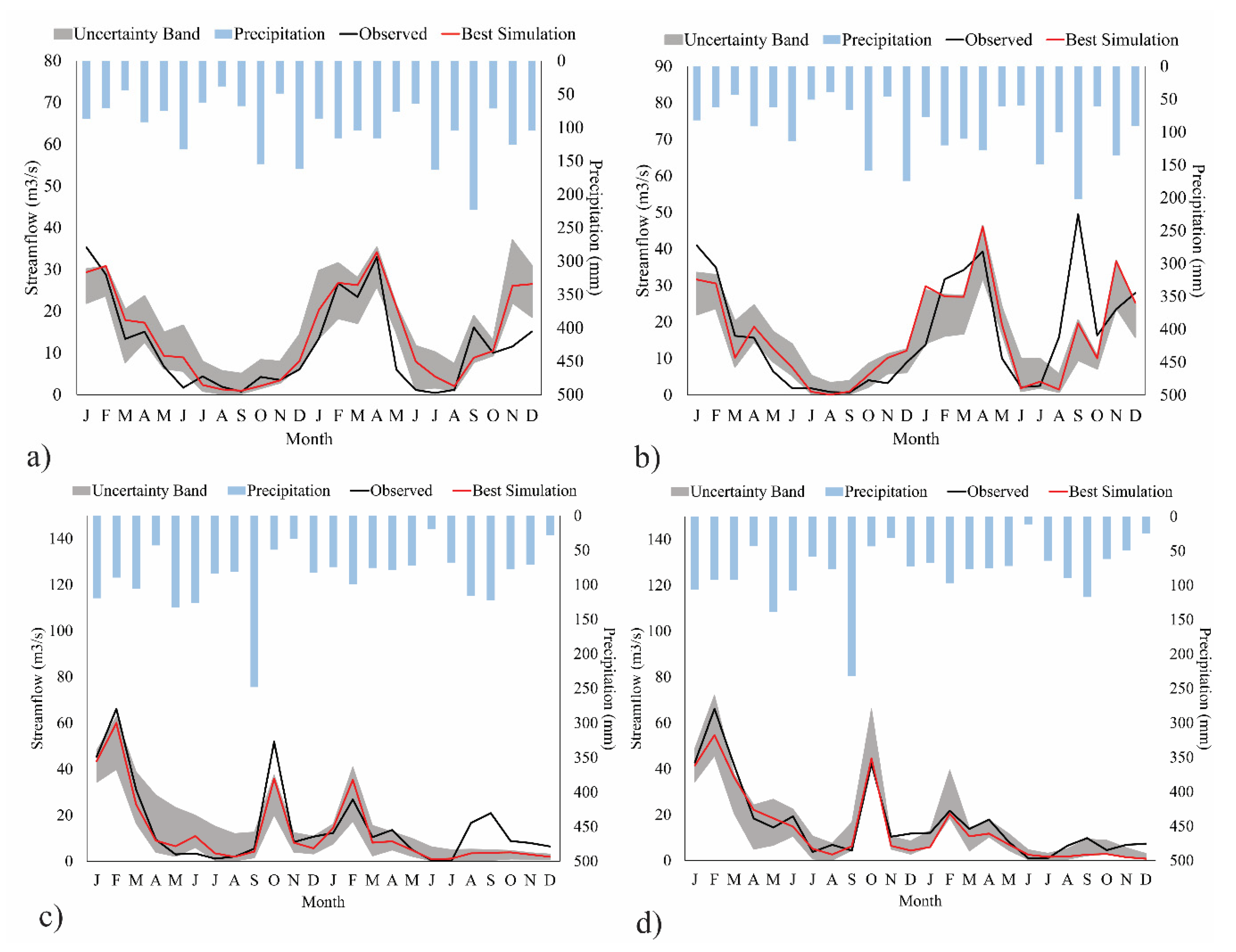
The results from our multi-year SWAT model calibration and validation demonstrate the effectiveness of incorporating gridded precipitation products into hydrological assessment models within the Atlantic Coastal Plain. Our model is the first of its kind to simultaneously assess streamflow, runoff, percolation, and sediment loss rate estimations using daily CFSR gridded climate data, and one of few studies that utilizes CFSR in Coastal Plain watersheds. Our model improves on previous rate estimations of runoff, percolation, and sediment loss by providing basin- and sub-watershed-specific estimates as opposed to estimates for the larger southeastern Atlantic Coastal Plain. Streamflow predictions at two gages resulted in acceptable results for the two-year calibration period (NSE = 0.67 and 0.60) and very good results during the two-year validation period (NSE = 0.84 and 0.91). SWAT model estimates for runoff, percolation, and sediment yield were all within reasonable ranges for this region of the Coastal Plain. However, estimates for the uncalibrated portions of the study area are more uncertain due to the inability to calibrate the model and tidal influence within these areas, due to the effects that tidal influence may have on ground- and surface-water dynamics. Additionally, we provide the first SWAT parameter assessment for the Black and NECF river basins. Our parameter sensitivity results highlight the need for detailed model refinement of initial parameters that relate to groundwater or aquifer properties at higher spatial resolutions for shallow water-table dominated hydrologic systems. Additionally, improvements are needed to the potential evapotranspiration estimates to further refine model predictions.
Long-term hydrologic models, as presented here, are a critical source of the scientifically-based information needed to make sound management decisions that sustain and protect the quality of regional water resources. The study results point to the utility of incorporating gridded climate products such as CFSR for hydrologic models in shallow-aquifer-dominated Coastal Plains systems where observational gage records are incomplete or inaccurately represent large-scale precipitation patterns. Our model provides the basis for future model development and parameterization refinement in the Black and NECF basins in support of regional watershed management plans. Further research is also needed to evaluate the effects of changes in climate or land use on dominant hydrologic processes within this region, as well as assessing model improvement through the incorporation of remotely sensed hydrologic data, such as ET or soil moisture.

Author Contributions

K.L.M. was responsible for conceptualization, methodology, formal analysis, original draft preparation, review and editing; N.G.P. was responsible for conceptualization, methodology, validation, review and editing. All authors have read and agreed to the published version of the manuscript.

Funding

This study was supported by a University of North Carolina Wilmington Sustainability Committee Green Initiative Fund award and an Ahuja Academy of Water Quality Fellowship to Kerry Mapes.

Acknowledgments

The authors would like to thank Roger Shew and Michael Mallin of the University of North Carolina Wilmington for their support and thoughtful feedback during the development and execution of this research. We would also like to thank the anonymous reviews and editor for their insightful feedback and suggestions for improvements to our publication.

Conflicts of Interest

The authors declare no conflict of interest.

References

  1. U.S. Environmental Protection Agency. Overview of watershed planning processes. In Handbook for Developing Watershed Plans to Restore and Protect Our Waters; U.S. Environmental Protection Agency: Washington, DC, USA, 2008; pp. 2.1–2.6. [Google Scholar]
  2. Wang, G.; Mang, S.; Cai, H.; Liu, S.; Zhang, Z.; Wang, L.; Innes, J. Integrated watershed management: Evolution, development and emerging trends. J. For. Res. 2016, 27, 967–994. [Google Scholar] [CrossRef] [Green Version]
  3. Wu, K.; Xu, Y.J. Evaluation of the applicability of the SWAT model for coastal watersheds. J. Am. Water Resour. Assoc. 2007, 42, 1247–1260. [Google Scholar] [CrossRef]
  4. Bosch, D.D.; Sheridan, J.M.; Batten, H.L.; Arnold, J.G. Evaluation of the SWAT model on a Coastal Plain agricultural watershed. Trans. ASAE 2004, 47, 1493–1506. [Google Scholar] [CrossRef]
  5. Le, A.M.; Pricope, N.G. Increasing the accuracy of runoff and streamflow simulation in the Nzoia Basin, Western Kenya, through the incorporation of satellite-derived CHIRPS data. Water 2017, 9, 114. [Google Scholar] [CrossRef]
  6. Arnold, J.G.; Srinivasan, R.; Muttiah, R.S.; Williams, J.R. Large area hydrologic modeling and assessment Part I: Model development. J. Am. Water Resour. Assoc. 1998, 34, 73–89. [Google Scholar] [CrossRef]
  7. Arnold, J.G.; Moriasi, D.N.; Gassman, P.W.; Abbaspour, K.C.; White, M.J.; Srinivasan, R.; Santhi, C.; Harmel, R.D.; van Griensven, A.; Van Liew, M.W.; et al. SWAT: Model use, calibration, and validation. Trans. ASABE 2012, 55, 1491–1508. [Google Scholar] [CrossRef]
  8. Neitsch, S.L.; Arnold, J.G.; Kiniry, J.R.; Williams, J.R. Soil and Water Assessment Tool Theoretical Documentation, version 2009; Texas Water Resources Institute, Texas A&M University: College Station, TX, USA, 2011; p. 647. [Google Scholar]
  9. Jha, M.; Gassman, P.W.; Secchi, S.; Gu, R.; Arnold, J. Effect of watershed subdivision on SWAT flow, sediment, and nutrient predictions. J. Am. Water Resour. Assoc. 2004, 40, 811–825. [Google Scholar] [CrossRef] [Green Version]
  10. Pandey, P.K.; Soupir, M.L.; Ikenberry, C. Modelling animal waste pathogen transport from agricultural land to streams. IOP Conf. Ser. Earth Environ. Sci. 2014, 19, 012014. [Google Scholar] [CrossRef] [Green Version]
  11. Rajib, M.A.; Merwade, V.; Yu, Z. Multi-objective calibration of a hydrologic model using spatially distributed remotely sensed/in-situ soil moisture. J. Hydrol. 2016, 536, 192–207. [Google Scholar] [CrossRef] [Green Version]
  12. Roth, V.; Lemann, T. Comparing CFSR and conventional weather data for discharge and soil loss modelling with SWAT in small catchments in the Ethiopian Highlands. Hydrol. Earth Syst. Sci. 2016, 20, 921–934. [Google Scholar] [CrossRef] [Green Version]
  13. Saleh, A.; Arnold, J.G.; Gassman, P.W.; Hauck, L.M.; Rosenthal, W.D.; Williams, J.R.; McFarland, A.M.S. Application of SWAT for the Upper North Bosque River Watershed. Trans. ASAE 2000, 43, 1077–1087. [Google Scholar] [CrossRef]
  14. Amatya, D.M.; Jha, M.K. Evaluating the SWAT model for a low-gradient forested watershed in coastal South Carolina. Trans. ASABE 2011, 54, 2151–2163. [Google Scholar] [CrossRef] [Green Version]
  15. Cho, J.; Bosch, D.; Vellidis, G.; Lowrance, R.; Strickland, T. Multi-site evaluation of hydrology component of SWAT in the coastal plain of southwest Georgia: Multi-site evaluation of SWAT hydrology. Hydrol. Proc. 2013, 27, 1691–1700. [Google Scholar] [CrossRef]
  16. Lam, Q.D.; Schmalz, B.; Fohrer, N. Modelling point and diffuse source pollution of nitrate in a rural lowland catchment using the SWAT model. Agric. Water Mgmt. 2010, 97, 317–325. [Google Scholar] [CrossRef]
  17. Rajbhandari, N.B.; Pradhan, S.; Luzio, M.D.; Kebede, A.; Baker, V. Identifying nutrient contributors in North Carolina Coastal Plain blackwater rivers. Am. J. Environ. Sci. 2015, 11, 313–324. [Google Scholar] [CrossRef] [Green Version]
  18. Samadi, S.Z. Assessing the sensitivity of SWAT physical parameters to potential evapotranspiration estimation methods over a coastal plain watershed in the southeastern United States. Hydrol. Res. 2017, 48, 395–415. [Google Scholar] [CrossRef]
  19. Samadi, S.; Tufford, D.L.; Carbone, G.J. Assessing parameter uncertainty of a semi-distributed hydrology model for a shallow aquifer dominated environmental system. J. Am. Water Resour. Assoc. 2017, 53, 1368–1389. [Google Scholar] [CrossRef]
  20. Bosch, D.D.; Arnold, J.G.; Volk, M.; Allen, P.M. Simulation of a low-gradient Coastal Plain watershed using the SWAT landscape model. Trans. ASABE 2010, 53, 1445–1456. [Google Scholar] [CrossRef]
  21. Fuka, D.R.; Walter, M.T.; MacAlister, C.; Degaetano, A.T.; Steenhuis, T.S.; Easton, Z.M. Using the Climate Forecast System Reanalysis as weather input data for watershed models. Hydrol. Proc. 2014, 28, 5613–5623. [Google Scholar] [CrossRef]
  22. Tomy, T.; Sumam, K.S. Determining the adequacy of CFSR data for rainfall-runoff modeling using SWAT. Procedia Technol. 2016, 24, 309–316. [Google Scholar] [CrossRef]
  23. Alemayehu, T.; Griensven, A.; Bauwens, W. Evaluating CFSR and WATCH data as input to SWAT for the estimation of the potential evapotranspiration in a data-scarce eastern-African catchment. J. Hydrol. Eng. 2015, 21, 05015028-1–05015028-16. [Google Scholar] [CrossRef]
  24. Dile, Y.; Srinivasan, R. Evaluation of CFSR climate data for hydrologic prediction in data-scarce watersheds: An application in the Blue Nile River Basin. J. Am. Water Resour. Assoc. 2014, 50, 1226–1241. [Google Scholar] [CrossRef]
  25. Grusson, Y.; Anctil, F.; Sauvage, S.; Sanchez Perez, J. Testing the SWAT model with gridded weather data of different spatial resolutions. Water 2017, 9, 54. [Google Scholar] [CrossRef] [Green Version]
  26. Burkholder, J.; Libra, B.; Weyer, P.; Heathcote, S.; Kolpin, D.; Thorne, P.S.; Wichman, M. Impacts of waste from concentrated animal feeding operations on water quality. Environ. Health Perspect. 2007, 115, 308–312. [Google Scholar] [CrossRef] [PubMed] [Green Version]
  27. Mallin, M.A. Impacts of industrial-scale swine and poultry production on rivers and estuaries. Am. Sci. 2000, 88, 26–37. [Google Scholar] [CrossRef]
  28. Mallin, M.A.; Cahoon, L.B. Industrialized animal production—A major source of nutrient and microbial pollution to aquatic ecosystems. Popul. Environ. 2003, 24, 369–385. [Google Scholar] [CrossRef]
  29. Mallin, M.A.; McIver, M.R.; Robuck, A.R.; Dickens, A.K. Industrial swine and poultry production causes chronic nutrient and fecal microbial stream pollution. Water Air Soil Pollut. 2015, 226. [Google Scholar] [CrossRef]
  30. Hupp, C.R. Hydrology, Geomorphology, and Vegetation of Coastal Plain Rivers in the Southeastern United States. Hydrol. Process. 2000, 14, 2991–3010. [Google Scholar] [CrossRef]
  31. Kroes, D.E.; Brinson, M.M. Occurrence of riverine wetlands on floodplains along a climatic gradient. Wetlands 2004, 24, 167–177. [Google Scholar] [CrossRef]
  32. Homer, C.; Dewitz, J.; Yang, L.; Jin, S.; Danielson, P.; Coulston, J.; Herold, N.; Wickham, J.; Megown, K. Completion of the 2011 National Land Cover Database for the conterminous United States–Representing a decade of land cover change information. Photogramm. Eng. Remote. Sens. 2015, 81, 345–354. [Google Scholar]
  33. U.S. Department of Agriculture National Agricultural Statistics Service. Livestock, Dairy, and Poultry Annual Statistical Bulletin. 2016. Available online: https://www.nass.usda.gov/Statistics_by_State/North_Carolina/Publications/Annual_Statistical_Bulletin/AgStat/Section04.pdf (accessed on 26 March 2019).
  34. Kottek, M.; Grieser, J.; Beck, C.; Rudolf, B.; Rubel, F. World map of the Köppen-Geiger climate classification updated. Meteorol. Z. 2006, 15, 259–263. [Google Scholar] [CrossRef]
  35. Arguez, A.; Durre, I.; Applequist, S.; Vose, R.S.; Squires, M.F.; Yin, X.; Heim, R.R.; Owen, T.W. NOAA’s 1981–2010 U.S. Climate Normals: An overview. Bull. Am. Meteorol. Soc. 2012, 93, 1687–1697. [Google Scholar] [CrossRef]
  36. National Oceanic and Atmospheric Administration. Continental United States Hurricane Impacts/Landfalls 1851–2016. Published 2017. Available online: http://www.aoml.noaa.gov/hrd/hurdat/uststorms.html (accessed on 8 February 2018).
  37. National Oceanic and Atmospheric Administration. Continental United States Tropical Storms Impacts/Landfalls 1851–1960, 1983–2016. Published 2017. Available online: http://www.aoml.noaa.gov/hrd/hurdat/uststorms.html (accessed on 8 February 2018).
  38. Winner, M.D.; Coble, R.W. Hydrogeological framework of the North Carolina Coastal Plain; UNITED STATES GOVERNMENT PRINTING OFFICE: Washington, DC, USA, 1996; 119p.
  39. Heath, R.C. Basic Elements of Ground-water Hydrology with Reference to Conditions in North Carolina; US Department of the Interior: Washington, DC, USA, 1980; 94p.
  40. Hardin, S.L.; Spruill, T.B. Ionic Composition and Nitrate Drainage Water from Fields Fertilized with Different Nitrogen Sources, Middle Swamp Watershed, North Carolina, August 2000–August 2001; U.S. Geological Survey Scientific Investigations; Report 2004-5123; US Department of the Interior, US Geological Survey: Raleigh, NC, USA, 2004; 14p. Available online: https://pubs.usgs.gov/sir/2004/5123/pdf/report.pdf (accessed on 2 February 2018).
  41. McMahon, G.; Lloyd, O.B. Water-quality assessment of the Albemarle-Pamlico Drainage Basin, North Carolina; Environmental Setting and Water-Quality Issues; U.S. Geological Survey: Raleigh, NC, USA, 1995.
  42. Environmental Systems Research Institute (ESRI). ArcGIS Release 10.3.1; Environmental Systems Research Institute (ESRI): Redlands, CA, USA, 2015. [Google Scholar]
  43. U.S. Geological Survey. The National Map: 3DEP Products and Services. 2017. Available online: https://nationalmap.gov/ (accessed on 8 February 2018).
  44. U.S. Geological Survey. The National Map: National Hydrography Dataset. 2017. Available online: https://nationalmap.gov/ (accessed on 8 February 2018).
  45. Lindsay, J.B. The practice of DEM stream burning revisited. Earth Surf. Proc. Landf. 2016, 41, 658–668. [Google Scholar] [CrossRef]
  46. O’Callaghan, J.F.; Mark, D.M. The extraction of drainage net- works from digital elevation data. Comput. Vision Graph. Image Process. 1984, 28, 328–344. [Google Scholar]
  47. U.S. Geological Survey. National Water Information System data available on the World Wide Web (USGS Water Data for the Nation). 2016. Available online: http://waterdata.usgs.gov/nwis/ (accessed on 8 February 2018).
  48. U.S. Geological Survey. NLCD 2011 Land Cover (2011 Edition, amended 2014)—National Geospatial Data Asset (NGDA) Land Use Land Cover: U.S. Geological Survey. 2014. Available online: https://www.mrlc.gov/data/nlcd-2011-land-cover-conus (accessed on 8 February 2018).
  49. Saha, S.; Moorthi, S.; Pan, H.-L.; Wu, X.; Wang, J.; Nadiga, S.; Tripp, P.; Kistler, R.; Woollen, J.; Behringer, D.; et al. The NCEP Climate Forecast System Reanalysis. Bull. Am. Meteorol. Soc. 2010, 91, 1015–1058. [Google Scholar] [CrossRef]
  50. U.S. Department of Agriculture, Soil Conservation Service. National Engineering Handbook; Hydrology Section 4; Chapter 19; U.S. Department of Agriculture, Soil Conservation Service: Washington, DC, USA, 1983.
  51. U.S. Department of Agriculture, Soil Conservation Service. National Engineering Handbook; Hydrology Section 4; Chapters 4–10; U.S. Department of Agriculture, Soil Conservation Service: Washington, DC, USA, 1972.
  52. U.S. Department of Agriculture, Soil Conservation Service. Urban Hydrology for Small Watersheds; Release 55; U.S. Department of Agriculture, Soil Conservation Service: Washington, DC, USA, 1986.
  53. Sloan, P.G.; Morre, I.D.; Coltharp, G.B.; Eigel, J.D. Modeling Surface and Subsurface Stormflow on Steeply-Sloping Forested Watersheds; Water Resources Inst. Report 142; University of Kentucky: Lexington, Kentucky, 1983. [Google Scholar]
  54. Schroeter, H.O.; Epp, R.P. Muskingum-Cunge: A practical alternative to the HYMO VSC Method for channel routing. Can. Water Resour. J. 1988, 13, 68–79. [Google Scholar] [CrossRef] [Green Version]
  55. Williams, J.R.; Berndt, H.D. Sediment yield prediction based on watershed hydrology. Trans. ASAE 1977, 20, 1100–1104. [Google Scholar] [CrossRef]
  56. Pricope, N.G. Assessment of spatial patterns of sediment transport and delivery for soil and water conservation programs. J. Spat. Hydrol. 2009, 9, 21–46. [Google Scholar]
  57. Lecce, S.A.; Gares, P.A.; Pease, P.P. Drainage ditches as sediment sinks on the Coastal Plain of North Carolina. Phys. Geogr. 2006, 27, 447–463. [Google Scholar] [CrossRef] [Green Version]
  58. Abbaspour, K.C. Swat-Cup2: SWAT Calibration and Uncertainty Programs Manual Version 2; Department of Systems Analysis, Integrated Assessment and Modelling (SIAM) Eawag. Swiss Federal Institute of Aquatic Science and Technology: Duebendorf, Switzerland, 2011; 106p. [Google Scholar]
  59. Abbaspour, K.C.; Johnson, C.A. Estimating uncertain flow and transport parameters using a sequential uncertainty fitting procedure. Vadose Zone J. 2004, 3, 13. [Google Scholar] [CrossRef]
  60. Abbaspour, K.C.; Yang, J.; Maximov, I.; Siber, R.; Bogner, K.; Mieleitner, J.; Zobrist, J.; Srinivasan, R. Modelling hydrology and water quality in the pre-alpine/alpine Thur watershed using SWAT. J. Hydrol. 2007, 333, 413–430. [Google Scholar] [CrossRef]
  61. Nash, J.E.; Sutcliffe, J.V. River flow forecasting through conceptual models part I—A discussion of principles. J. Hydrol. 1970, 10, 282–290. [Google Scholar] [CrossRef]
  62. Abbaspour, K.C.; Rouholahnejad, E.; Vaghefi, S.; Srinivasan, R.; Yang, H.; Kløve, B. A continental-scale hydrology and water quality model for Europe: Calibration and uncertainty of a high-resolution large-scale SWAT model. J. Hydrol. 2015, 524, 733–752. [Google Scholar] [CrossRef] [Green Version]
  63. Coes, A.L.; Spruill, T.B.; Thomasson, M.J. Multiple-method estimation of recharge rates at diverse locations in the North Carolina Coastal Plain, USA. Hydrogeol. J. 2007, 15, 773–788. [Google Scholar] [CrossRef]
  64. Endale, D.M. Sediment loss and runoff from cropland in a southeast Atlantic Coastal Plain landscape. Trans. ASABE 2014, 57, 1611–1626. [Google Scholar] [CrossRef]
  65. Samadi, S.Z.; Meadows, M.E. The transferability of terrestrial water balance components under uncertainty and nonstationarity: A case study of the Coastal Plain watershed in the Southeastern USA. River Res. Appl. 2017, 33, 796–808. [Google Scholar] [CrossRef]
  66. Wilder, H.B.; Robison, T.M.; Lindskov, K.L. Water Resources of Northeast North Carolina; U.S. Geological Survey Water-Resources Investigations; U.S. Geological Survey Water Resources Division: Raleigh, NC, USA, 1978; pp. 77–81.
  67. Hardin, S.L.; Fine, J.M.; Spruill, T.B. Hydrogeology and Ground-Water Quality of Brunswick County, North Carolina; Water Resources Investigation Report No. 03–4051; US Department of the Interior, US Geological Survey: Raleigh, NC, USA, 2003. [CrossRef]
  68. Bain, G.L. Geology and Ground-Water Resources of New Hanover County, North Carolina; U.S. Geological Survey Ground Water Bulletin; U.S. Geological Survey: Raleigh, NC, USA, 1970; 94p.
  69. Griffin, M.P.; Callahan, T.J.; Vulava, V.M.; Williams, T.M. Storm-event flow pathways in lower coastal plain forested watersheds of the southeastern United States. Water Resour. Res. 2014, 50, 8265–8280. [Google Scholar] [CrossRef] [Green Version]
  70. Sanford, W.E.; Selnick, D.L. Estimation of Evapotranspiration across the Conterminous United States Using a Regression With Climate and Land-Cover Data. JAWRA 2013, 49, 217–230. [Google Scholar]
  71. Baffaut, C.; John Sadler, E.; Ghidey, F.; Anderson, S.H. Long-term agroecosystem research in the Central Mississippi River Basin: SWAT simulation of flow and water quality in the Goodwater Creek Experimental Watershed. J. Environ. Qual. 2015, 44, 84. [Google Scholar] [CrossRef]
  72. U.S. Natural Resources Conservation Service. Sediment loss from water erosion. In Model Simulation of Soil Loss, Nutrient Loss, and Change in Soil Organic Carbon Associated with Crop Production; U.S. Department of Agriculture: Washington, DC, USA, 2006; pp. 73–74. [Google Scholar]
  73. Lecce, S.A.; Pease, P.P.; Gares, P.A.; Wang, J. Seasonal controls on sediment delivery in a small coastal plain watershed, North Carolina, USA. Geomorphology 2006, 73, 246–260. [Google Scholar] [CrossRef]
  74. Simmons, C.E. Sediment Characteristics of Streams in the Eastern Piedmont and Western Coastal Plain Regions of North Carolina; U.S. Government Printing Office: Washington, DC, USA, 1976; 41p. Available online: https://pubs.er.usgs.gov/publication/wsp1798O (accessed on 7 March 2019).
  75. Carter, L.; Terando, A.; Dow, K.; Hiers, K.; Kunkel, K.E.; Lascurain, A.; Marcy, D.; Osland, M.; Schramm, P. Southeast. In Impacts, Risks, and Adaptation in the United States: Fourth National Climate Assessment; Reidmiller, D.R., Avery, C.W., Easterling, D.R., Kunkel, K.E., Lewis, K.L.M., Maycock, T.K., Stewart, B.C., Eds.; U.S. Global Change Research Program: Washington, DC, USA, 2018; Volume II, pp. 743–808. [Google Scholar] [CrossRef]
  76. Nearing, M.A.; Pruski, F.F.; O’Neal, M.R. Expected climate change impacts on soil erosion rates: A review. J. Soil Water Cons. 2003, 59, 43–50. [Google Scholar]
  77. Immerzeel, W.W.; Droogers, P. Calibration of a distributed hydrologic model based on satellite evapotranspiration. J. Hydrol. 2008, 349, 411–424. [Google Scholar] [CrossRef]
Figure 1. The 4076.5 km2 Black and 4510.0 km2 Northeast Cape Fear Basins used in the Soil and Water Assessment Tool. Modeled streamflow was compared to data from the United States Geological Survey (USGS) gaging stations at Chinquapin and Tomahawk. See Table 1 for an explanation of the land-use abbreviations.
Hydrology 07 00021 g001
Figure 2. Monthly streamflow calibration and validation using SUFI-2, Northeast Cape Fear basin. The calibration period (January 2007–December 2008) is shown for Chinquapin station (a) and Tomahawk station (b). The validation period (January 2010 to December 2011) is shown for Chinquapin station (c) and Tomahawk station (d). The uncertainty band is depicted by a light gray band, which represents the 95PPU or p-factor of streamflow calibration. See Table 6 for model performance statistics.
Hydrology 07 00021 g002
Figure 3. Yearly average estimates of surface runoff (SURQ) and percolation (PERC) from the validation period of 2010–2011 using SWAT-CUP.
Hydrology 07 00021 g003
Figure 4. Yearly average estimates of Sediment Yield (SYLD) from the validation period of 2010–2011 using SWAT-CUP.
Hydrology 07 00021 g004
Table 1. National Land Cover Dataset (NLCD) with the corresponding Soil and Water Assessment Tool (SWAT) land-use classes in the Black and Northeast Cape Fear basins.
Land Use ClassPercent Area
NLCDSWATBlackNECF
Open WaterWATR0.780.75
Developed, Open SpaceURLD3.963.12
Developed, Low IntensityURMD1.411.40
Developed, Medium IntensityURHD0.260.39
Developed, High IntensityUIDU0.080.13
Barren LandSWRN0.380.40
Deciduous ForestFRSD0.280.13
Evergreen ForestFRSE15.1216.74
Mixed ForestFRST2.412.16
Shrub/scrubRNGB13.8411.95
Grassland/HerbaceousRNGE4.383.75
Pasture/HayHAY0.620.09
Cultivated CropsAGRR30.2023.43
Woody WetlandsWETF24.0333.54
Emergent Herbaceous WetlandsWETN2.252.02
Table 2. State Soil Geographic Data (STATSGO) soil types in the Black and Northeast Cape Fear basins.
MUIDHydrologic GroupPercent Area
BlackNECF
NC001D16.976.68
NC003C0.200.11
NC010C0.10<0.01
NC011A<0.010.38
NC019A1.7110.01
NC024D<0.011.13
NC028D<0.010.86
NC030B0.520.56
NC033D2.6124.01
NC034B1.587.59
NC035B31.2623.13
NC038A19.3416.32
NC039B7.917.43
NC040A9.840.65
NC044B<0.011.14
NC049D5.97<0.01
NC050A1.84<0.01
NCWD0.15<0.01
Table 3. Record of data used in this study, sources, and spatial and temporal resolutions if applicable.
TypeDatasetYearFormatResolution
SpatialTemporal
Digital Elevation ModelUSGS 3D Elevation Program2017Raster10 m
Stream centerlinesFlood Risk Information System2012–2015Vector
Watershed boundariesUSGS Watershed Boundaries Dataset2008Vector
Land use/land coverNational Land Cover Database2011Raster30 m
SoilUSGS State Soil Survey Geographic (STATSGO)1995Raster250 m
ClimateNCEP-CFSR2000–2011Text0.5°Daily
Stream flowUSGS National Water Information System2000–2011Spreadsheet Monthly
Table 4. Calibration parameters and initial ranges used in SWAT-CUP. The letter “r” indicates a relative change in value, while the letter “v” indicates a replacement. Parameter descriptions are available in Neitsch et al. [8].
SWAT ParameterDescriptionAbsolute ValuesInitial Range
r_CN2.mgtCurve number, moisture condition II35–98−0.2–0.2
v_ALPHA_BF.gwBaseflow recession constant, days0–10–1
v_GW_DELAY.gwGroundwater delay, days0–50030–450
v_GWQMIN.gwThreshold water depth in shallow aquifer for return to reach to occur (mm)0–50000–5000
v_CH_N2.rteMain channel Manning’s “n”−0.01–0.30–0.3
r_SOL_K().solSaturated hydraulic conductivity, mm/h0–2000−0.8–0.8
v_ESCO.hruSoil evaporation compensation factor0–10.8–1
r_SOL_AWC().solAvailable soil water capacity, mmH2O per mm of soil0–1−0.2–0.4
v_GW_REVAP.gwGroundwater re-evaporation coefficient0.02–0.20.02–0.2
r_OV_N.hruManning’s “n” value for overland flow0.01–30−0.2–0
v_GWHT.gwInitial groundwater height (m)0–250–25
r_SOL_BD().solMoist bulk density (Mg/m3 or g/cm3)0.9–2.5−0.2–0.2
r_RCHRG_DP.gwDeep aquifer percolation fraction0–1−0.8–0.8
r_GW_SPYLD.gwSpecific yield of the shallow aquifer (m3/m3)0–0.4−0.5–0.5
v_LAT_TTIME.hruLateral flow travel time (days)0–1800–180
r_EPCO.hruPlant uptake compensation factor0–1−0.5–0.5
r_SLSUBBSN.hruAverage slope length (m)10–150−0.6–0.6
Table 5. Statistics for the Climate Forecast System Reanalysis (CFSR) precipitation data used in SWAT. Because there was some variation in total monthly precipitation for the 58 watersheds used in this study, the values reported are an average of all watersheds during each stated time period.
YearAvg (mm)Min (mm)Max (mm)
20079997371105
2008130510161366
201011479641289
20118767171095
Calibration (2007 and 2008)11527371366
Validation (2010 and 2011)10127171289
Table 6. SWAT Calibration and Uncertainty Program (SWAT-CUP) objective function results for the calibration and validation periods.
Calibration (2007 and 2008)
Gagep-factorr-factorR2NSE
Chinquapin0.710.860.760.67
Tomahawk0.540.580.610.60
Validation (2010 and 2011)
Gagep-factorr-factorR2NSE
Chinquapin0.710.700.870.84
Tomahawk0.830.680.940.91
Table 7. Parameter best value estimates and sensitivity rankings using SUFI-2 in SWAT-CUP for the Black and Northeast Cape Fear basins for the validation years 2010–2011.
ChinquapinTomahawk
ParameterSensitivityBest ValueSensitivityBest Value
v_ALPHA_BF.gw10.5450.38
r_OV_N.hru20.0018−0.032
r_SOL_K().sol30.493−0.65
r_GW_SPYLD.gw40.2240.53
r_SOL_AWC().sol50.6711−0.001
v_LAT_TTIME.hru6148.81982.27
v_GW_REVAP.gw70.2110.20
r_EPCO.hru80.57160.06
v_GWHT.gw92.6521.75
v_GWQMIN.gw100.9673.11
r_CN2.mgt11−0.21130.04
r_RCHRG_DP.gw12−0.5810−0.70
v_ESCO.hru130.7760.71
r_SLSUBBSN.hru14−0.09150.20
r_SOL_BD().sol150.22140.07
v_CH_N2.rte160.15170.23
v_GW_DELAY.gw1713.751267.11

