Assessing Digital Soil Inventories for Predicting Streamflow in the Headwaters of the Blue Nile

 , ,
, , 
Abstract
1. Introduction
2. Materials and Methods
2.1. Study Area
2.2. Data
2.2.1. Hydrometeorological Data
2.2.2. Spatial Data
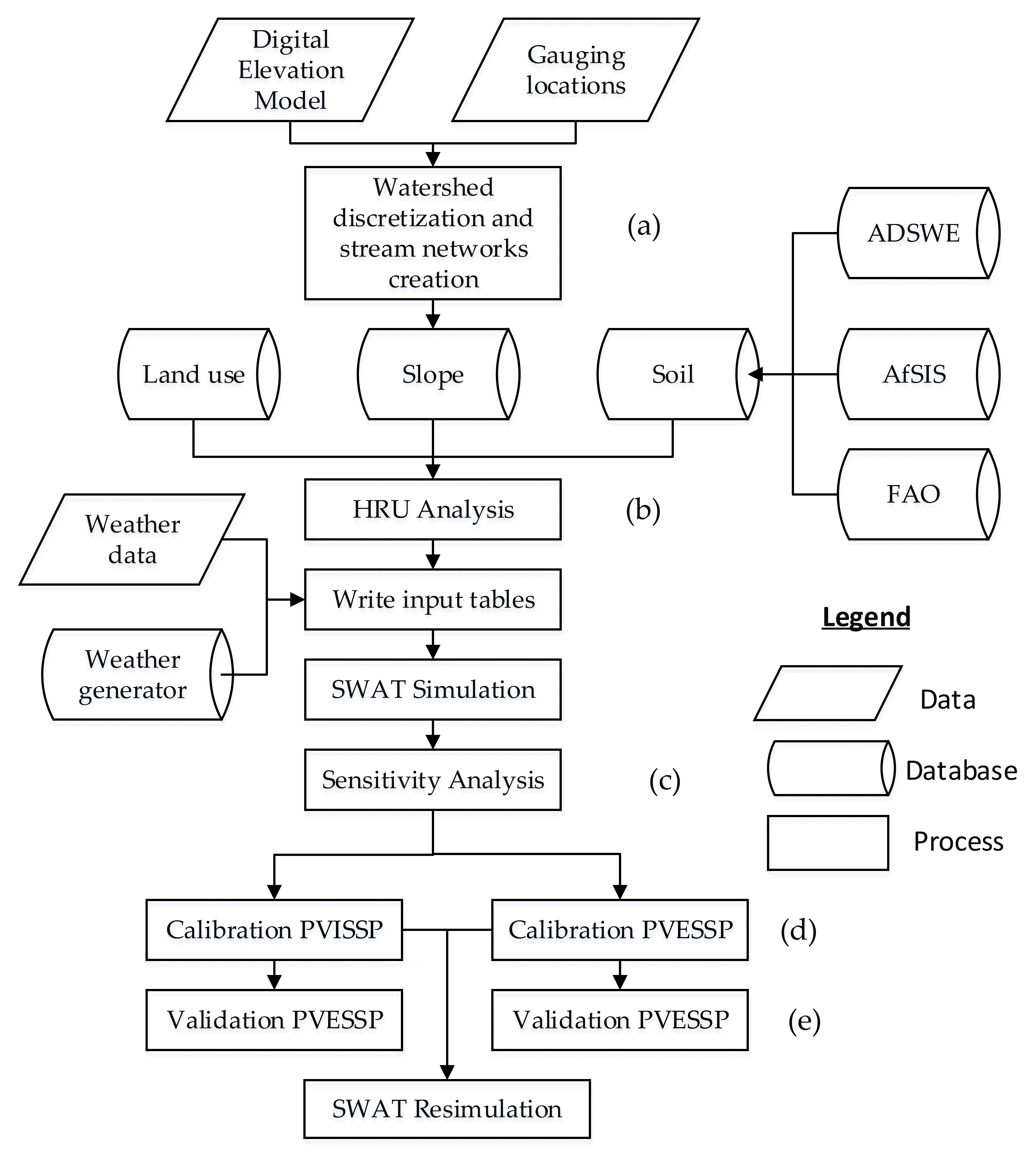
2.3. Analysis
2.3.1. Soil and Water Assessment Tool (SWAT) Model Description
2.3.2. Model Setup and Calibration
2.3.3. Model Performance Evaluation
3. Results
3.1. Comparing Model Components before Calibration
3.2. Sensitivity Analysis
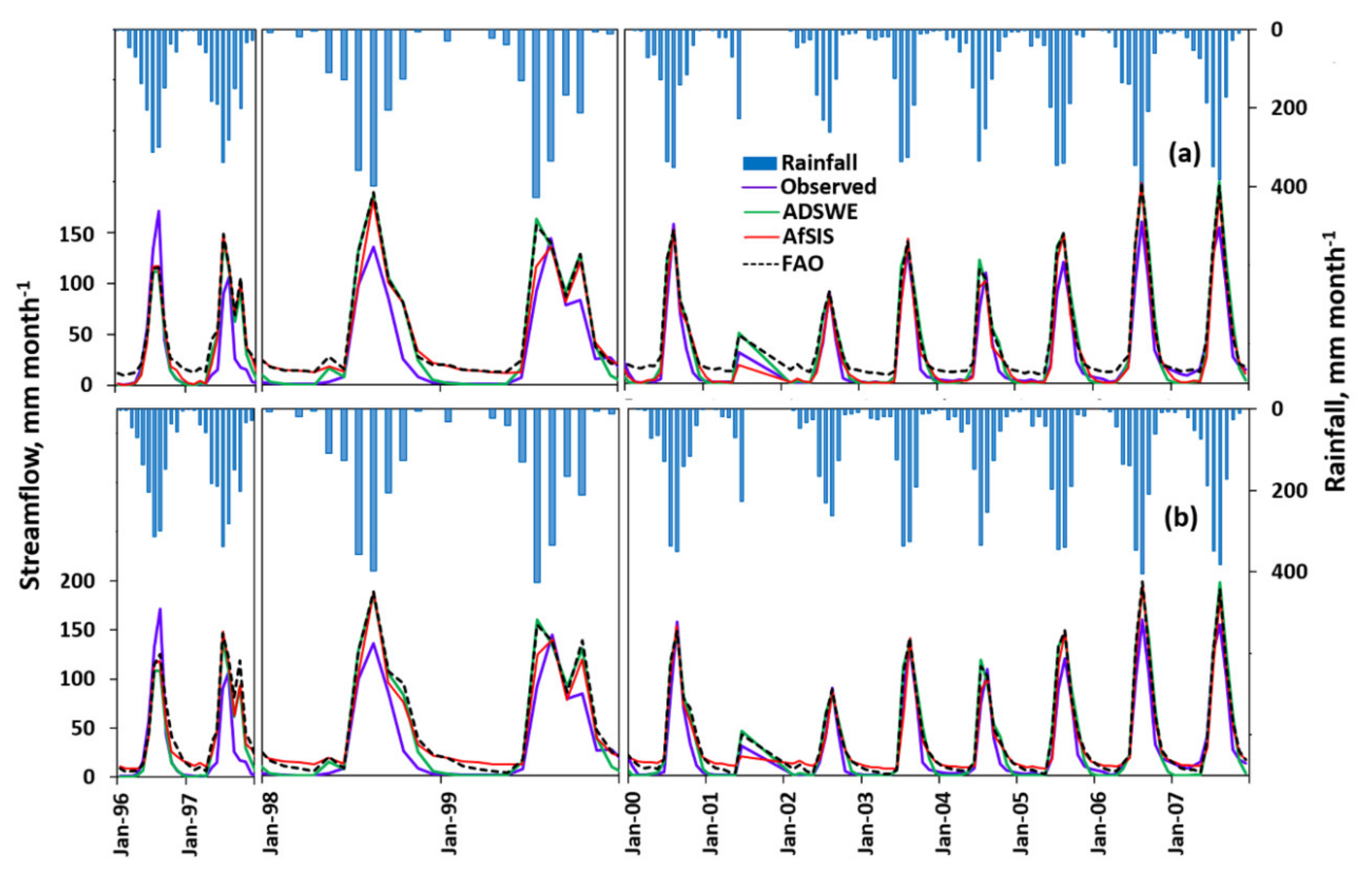
3.3. Comparing Model Components for the Period of Calibration
3.3.1. General Observations
3.3.2. The Rib Watershed
3.3.3. The Gomit Watershed
4. Discussion
5. Conclusions
Supplementary Materials
Author Contributions
Funding
Acknowledgments
Conflicts of Interest
References
- Lin, H.; Wheeler, D.; Bell, J.; Wilding, L. Assessment of soil spatial variability at multiple scales. Ecol. Model. 2005, 182, 271–290. [Google Scholar] [CrossRef]
- Burrough, P.A. Soil variability: A late 20th century view. Soils Fert. 1993, 56, 529–562. [Google Scholar]
- Foussereau, X.; Hornsby, A.; Brown, R. Accounting for variability within map units when linking a pesticide fate model to soil survey. Geoderma 1993, 60, 257–276. [Google Scholar] [CrossRef]
- Wilding, L.P.; Bouma, J.; Goss, D.W. Impact of spatial variability on interpretive modeling. Quant. Modeling Soil Form. Process. 1994, 10, 61–75. [Google Scholar] [CrossRef]
- FAO. FAO Soils Portal. FAO SOILS PORTAL. Available online: http://www.fao.org/soils-portal/soil-survey/soil-maps-and-databases/en/ (accessed on 24 December 2019).
- DeVantier, B.A.; Feldman, A.D. Review of GIS applications in hydrologic modeling. J. Water Resour. Plan. Manag. 1993, 119, 246–261. [Google Scholar] [CrossRef]
- Cho, Y.; Engel, B.A. Spatially distributed long-term hydrologic simulation using a continuous SCS CN method-based hybrid hydrologic model. Hydrol. Process. 2018, 32, 904–922. [Google Scholar] [CrossRef]
- Singh, V.P. Computer Models of Watershed Hydrology; Water Resources Publications LLC: Highlands Ranch, CO, USA, 1995; Volume 1130. [Google Scholar]
- Beven, K.J. Rainfall-Runoff Modelling: The Primer; John Wiley & Sons: Chichester, UK, 2011. [Google Scholar]
- Jajarmizadeh, M.; Harun, S.; Salarpour, M. A review on theoretical consideration and types of models in hydrology. J. Environ. Sci. Technol. 2012, 5, 249–261. [Google Scholar] [CrossRef]
- Arnold, J.G.; Srinivasan, R.; Muttiah, R.S.; Williams, J.R. Large area hydrologic modeling and assessment part I: Model development. Jawra J. Am. Water Resour. Assoc. 1998, 34, 73–89. [Google Scholar] [CrossRef]
- Singh, V.P.; Frevert, D.K. Watershed Models; CRC Press, Taylor & Francis Group: Boca Raton, FL, USA, 2005. [Google Scholar]
- Pechlivanidis, I.; Jackson, B.; McIntyre, N.; Wheater, H. Catchment scale hydrological modelling: A review of model types, calibration approaches and uncertainty analysis methods in the context of recent developments in technology and applications. Glob. Nest J. 2011, 13, 193–214. [Google Scholar]
- Romanowicz, A.A.; Vanclooster, M.; Rounsevell, M.; La Junesse, I. Sensitivity of the SWAT model to the soil and land use data parametrisation: A case study in the Thyle catchment, Belgium. Ecol. Model. 2005, 187, 27–39. [Google Scholar] [CrossRef]
- Earls, J.; Dixon, B. A comparative study of the effects of input resolution on the SWAT model. WIT Trans. Ecol. Environ. 2005, 83, 213–222. [Google Scholar]
- Dixon, B.; Earls, J. Effects of urbanization on streamflow using SWAT with real and simulated meteorological data. Appl. Geogr. 2012, 35, 174–190. [Google Scholar] [CrossRef]
- Faramarzi, M.; Abbaspour, K.C.; Vaghefi, S.A.; Farzaneh, M.R.; Zehnder, A.J.; Srinivasan, R.; Yang, H. Modeling impacts of climate change on freshwater availability in Africa. J. Hydrol. 2013, 480, 85–101. [Google Scholar] [CrossRef]
- Shen, Z.; Chen, L.; Liao, Q.; Liu, R.; Huang, Q. A comprehensive study of the effect of GIS data on hydrology and non-point source pollution modeling. Agric. Water Manag. 2013, 118, 93–102. [Google Scholar] [CrossRef]
- Zhang, P.; Liu, R.; Bao, Y.; Wang, J.; Yu, W.; Shen, Z. Uncertainty of SWAT model at different DEM resolutions in a large mountainous watershed. Water Res. 2014, 53, 132–144. [Google Scholar] [CrossRef] [PubMed]
- Chaubey, I.; Cotter, A.; Costello, T.; Soerens, T. Effect of DEM data resolution on SWAT output uncertainty. Hydrol. Process. Int. J. 2005, 19, 621–628. [Google Scholar] [CrossRef]
- Kuo, W.L.; Steenhuis, T.S.; McCulloch, C.E.; Mohler, C.L.; Weinstein, D.A.; DeGloria, S.D.; Swaney, D.P. Effect of grid size on runoff and soil moisture for a variable-source-area hydrology model. Water Resour. Res. 1999, 35, 3419–3428. [Google Scholar] [CrossRef]
- Peschel, J.M.; Haan, P.K.; Lacey, R.E. A SSURGO pre-processing extension for the ArcView Soil and Water Assessment Tool. In Proceedings of the 2003 ASAE Annual Meeting, Las Vegas, NV, USA, 27–30 July 2003; pp. 1–17. [Google Scholar]
- Levick, L.; Semmens, D.; Guertin, D.; Burns, I.; Scott, S.; Unkrich, C.; Goodrich, D. Adding Global Soils Data to the Automated Geospatial Watershed Assessment Tool (AGWA). In Proceedings of the 2nd International Symposium on Transboundary Waters Management, Tucson, AZ, USA, 16–19 November 2004; pp. 16–19. [Google Scholar]
- Chaplot, V. Impact of DEM mesh size and soil map scale on SWAT runoff, sediment, and NO3–N loads predictions. J. Hydrol. 2005, 312, 207–222. [Google Scholar] [CrossRef]
- Prasanna, H.; Mulla, D. Scale effects of STATSGO vs. SSURGO soil databases on water quality predictions. In Proceedings of the Watershed management to meet water quality standards and emerging (total maximum daily load)(TMDL), Atlanta, GA, USA, 5–9 March 2005; pp. 5–9. [Google Scholar]
- Wang, X.; Melesse, A.M. Effects of STATSGO and SSURGO as inputs on SWAT model’s snowmelt simulation. JAWRA J. Am. Water Resour. Assoc. 2006, 42, 1217–1236. [Google Scholar] [CrossRef]
- Geza, M.; McCray, J.E. Effects of soil data resolution on SWAT model stream flow and water quality predictions. J. Environ. Manag. 2008, 88, 393–406. [Google Scholar] [CrossRef]
- Mukundan, R.; Radcliffe, D.; Risse, L. Spatial resolution of soil data and channel erosion effects on SWAT model predictions of flow and sediment. J. Soil Water Conserv. 2010, 65, 92–104. [Google Scholar] [CrossRef]
- Singh, H.V.; Kalin, L.; Srivastava, P. Effect of soil data resolution on identification of critical source areas of sediment. J. Hydrol. Eng. 2011, 16, 253–262. [Google Scholar] [CrossRef]
- Boluwade, A.; Madramootoo, C. Modeling the impacts of spatial heterogeneity in the castor watershed on runoff, sediment, and phosphorus loss using SWAT: I. Impacts of spatial variability of soil properties. WaterAir Soil Pollut. 2013, 224, 1692. [Google Scholar] [CrossRef] [PubMed]
- Bossa, A.; Diekkrüger, B.; Igué, A.; Gaiser, T. Analyzing the effects of different soil databases on modeling of hydrological processes and sediment yield in Benin (West Africa). Geoderma 2012, 173, 61–74. [Google Scholar] [CrossRef]
- Adem, A.A.; Aynalem, D.W.; Tilahun, S.A.; Steenhuis, T.S. Predicting Reference Evaporation for the Ethiopian Highlands. J. Water Resour. Prot. 2017, 9, 1244–1269. [Google Scholar] [CrossRef]
- Moges, D.M.; Bhat, H.G. Integration of geospatial technologies with RUSLE for analysis of land use/cover change impact on soil erosion: Case study in Rib watershed, north-western highland Ethiopia. Environ. Earth Sci. 2017, 76, 765. [Google Scholar] [CrossRef]
- Neitsch, S.L.; Arnold, J.G.; Kiniry, J.R.; Williams, J.R. Soil and water assessment tool theoretical documentation version 2009; Texas Water Resources Institute: College Station, TX, USA, September 2011. [Google Scholar]
- Adem, A.A.; Tilahun, S.A.; Ayana, E.K.; Worqlul, A.W.; Assefa, T.T.; Dessu, S.B.; Melesse, A.M. Climate Change Impact on Sediment Yield in the Upper Gilgel Abay Catchment, Blue Nile Basin, Ethiopia. Landsc. Dyn. Soils Hydrol. Process. Varied Clim. 2016, 615–644. [Google Scholar] [CrossRef]
- Adem, A.A.; Tilahun, S.A.; Ayana, E.K.; Worqlul, A.W.; Assefa, T.T.; Dessu, S.B.; Melesse, A.M. Climate change impact on stream flow in the upper Gilgel Abay Catchment, Blue Nile Basin, Ethiopia. Landsc. Dyn. Soils Hydrol. Process. Varied Clim. 2016, 645–673. [Google Scholar] [CrossRef]
- ASF. ALOS PALSAR_Radiometric_Terrain_Corrected_low_res; Includes Material © JAXA/METI 2007. Available online: https://vertex.daac.asf.alaska.edu (accessed on 23 January 2020).
- ADSWE. Tana Sub Basin Land Use Planning and Environmental Study Project, Technical Report I: Soil Survey; ADSWE, LUPESP: Bahir Dar, Ethiopia, 2015; Volume 1, p. 151. [Google Scholar]
- Hengl, T.; Heuvelink, G.B.; Kempen, B.; Leenaars, J.G.; Walsh, M.G.; Shepherd, K.D.; Sila, A.; MacMillan, R.A.; de Jesus, J.M.; Tamene, L. Mapping soil properties of Africa at 250 m resolution: Random forests significantly improve current predictions. PLoS ONE 2015, 10, 1–26. [Google Scholar] [CrossRef]
- Nachtergaele, F.; van Velthuizen, H.; Verelst, L.; Batjes, N.; Dijkshoorn, K.; van Engelen, V.; Fischer, G.; Jones, A.; Montanarella, L.; Petri, M. Harmonized world soil database (version 1.1); FAO: Rome, Italy, March 2009; p. 43. [Google Scholar]
- MoWR. Abbay River Basin Integrated Development Mater Plan Project: Land Resources Development, Part 1, Reconnaissance Soils Survey Report; Ministry of Water Resources (MoWR): Addis Ababa, Ethiopia, 1998; Volume 8, Phase 2.
- Kayitakire, F.; Hamel, C.; Defourny, P. Retrieving forest structure variables based on image texture analysis and IKONOS-2 imagery. Remote Sens. Environ. 2006, 102, 390–401. [Google Scholar] [CrossRef]
- Lu, D.; Weng, Q. A survey of image classification methods and techniques for improving classification performance. Int. J. Remote Sens. 2007, 28, 823–870. [Google Scholar] [CrossRef]
- Blaschke, T. Object based image analysis for remote sensing. ISPRS J. Photogramm. Remote Sens. 2010, 65, 2–16. [Google Scholar] [CrossRef]
- Arnold, J.G.; Moriasi, D.N.; Gassman, P.W.; Abbaspour, K.C.; White, M.J.; Srinivasan, R.; Santhi, C.; Harmel, R.; Van Griensven, A.; Van Liew, M.W. SWAT: Model use, calibration, and validation. Trans. Asabe 2012, 55, 1491–1508. [Google Scholar] [CrossRef]
- Douglas-Mankin, K.; Srinivasan, R.; Arnold, J. Soil and Water Assessment Tool (SWAT) model: Current developments and applications. Trans. Asabe 2010, 53, 1423–1431. [Google Scholar] [CrossRef]
- Neitsch, S.; Arnold, J.; Kiniry, J.; Williams, J. SWAT User Manual (Version 2009). Tex. Water Resour. Inst. Tech. Rep. 2005. [Google Scholar]
- Azizian, A.; SHOKOOHI, A. DEM resolution and stream delineation threshold effects on the results of geomorphologic-based rainfall runoff models. Turk. J. Eng. Environ. Sci. 2014, 38, 64–78. [Google Scholar] [CrossRef]
- Dixon, B.; Earls, J. Resample or not?! Effects of resolution of DEMs in watershed modeling. Hydrol. Process. 2009, 23, 1714–1724. [Google Scholar] [CrossRef]
- Singh, G.; Kumar, E. Input data scale impacts on modeling output results: A review. J. Spat. Hydrol. 2017, 13. [Google Scholar]
- Camargos, C.; Julich, S.; Houska, T.; Bach, M.; Breuer, L. Effects of Input Data Content on the Uncertainty of Simulating Water Resources. Water 2018, 10, 621. [Google Scholar] [CrossRef]
- Abbaspour, K.C. SWAT-CUP4: SWAT Calibration and Uncertainty Programs—A User Manual. Swiss Fed. Inst. Aquat. Sci. Technol. Eawag 2011, 21. [Google Scholar]
- Setegn, S.G. Hydrological and Sediment Yield Modelling in Lake Tana Basin, Blue Nile Ethiopia. Ph.D. Thesis, Royal Institute of Technology (KTH), Stockholm, Sweden, 2008. [Google Scholar]
- Krause, P.; Boyle, D.; Bäse, F. Comparison of different efficiency criteria for hydrological model assessment. Adv. Geosci. 2005, 5, 89–97. [Google Scholar] [CrossRef]
- Moriasi, D.N.; Arnold, J.G.; Van Liew, M.W.; Bingner, R.L.; Harmel, R.D.; Veith, T.L.J. Model evaluation guidelines for systematic quantification of accuracy in watershed simulations. Trans. Am. Soc. Agric. Biol. Eng. 2007, 50, 885–900. [Google Scholar] [CrossRef]
- Elshamy, M.E. Assessing the hydrological performance of the Nile Forecast System in long term simulations. Nile Water Sci. Eng. Mag. 2008, 1, 22–36. [Google Scholar]
- Nash, J.E.; Sutcliffe, J.V. River flow forecasting through conceptual models part I—A discussion of principles. J. Hydrol. 1970, 10, 282–290. [Google Scholar] [CrossRef]
- Legates, D.R.; McCabe, G.J. Evaluating the use of “goodness-of-fit” measures in hydrologic and hydroclimatic model validation. Water Resour. Res. 1999, 35, 233–241. [Google Scholar] [CrossRef]
- Skaik, Y.A. The bread and butter of statistical analysis “t-test”: Uses and misuses. Pak. J. Med. Sci. 2015, 31, 1558–1559. [Google Scholar] [CrossRef] [PubMed]
- Adem, A.A.; Aynalem, D.W.; Tilahun, S.A.; Mekuria, W.; Azeze, M.; Steenhuis, T.S. Runoff response and the associated soil and nutrient loss in two northwestern Ethiopian highland watersheds. In Proceedings of the International Conference on the Advancements of Sceince and Technology (ICAST-CWRE-2017), Bahir Dar, Ethiopia, May 2017; pp. 30–35. [Google Scholar]
- Dessie, M.; Verhoest, N.E.; Admasu, T.; Pauwels, V.R.; Poesen, J.; Adgo, E.; Deckers, J.; Nyssen, J. Effects of the floodplain on river discharge into Lake Tana (Ethiopia). J. Hydrol. 2014, 519, 699–710. [Google Scholar] [CrossRef]
- Wale, A.; Rientjes, T.; Dost, R.; Gieske, A. Hydrological balance of Lake Tana Upper Blue Nile basin, Ethiopia. In Proceedings of the workhop on hydrology and ecology of the Nile river basin under extreme conditions, Addis Ababa, Ethiopia, 16–19 June 2008; pp. 159–180. [Google Scholar]
- Zimale, F.; Moges, M.; Alemu, M.; Ayana, E.; Demissie, S.; Tilahun, S.; Steenhuis, T. Calculating the sediment budget of a tropical lake in the Blue Nile basin: Lake Tana. SOIL Discuss. 2016. [Google Scholar] [CrossRef]


| Watershed | Soil Inventory | Soil Textural Class | ||
|---|---|---|---|---|
| Clay % | Clay Loam % | Others % | ||
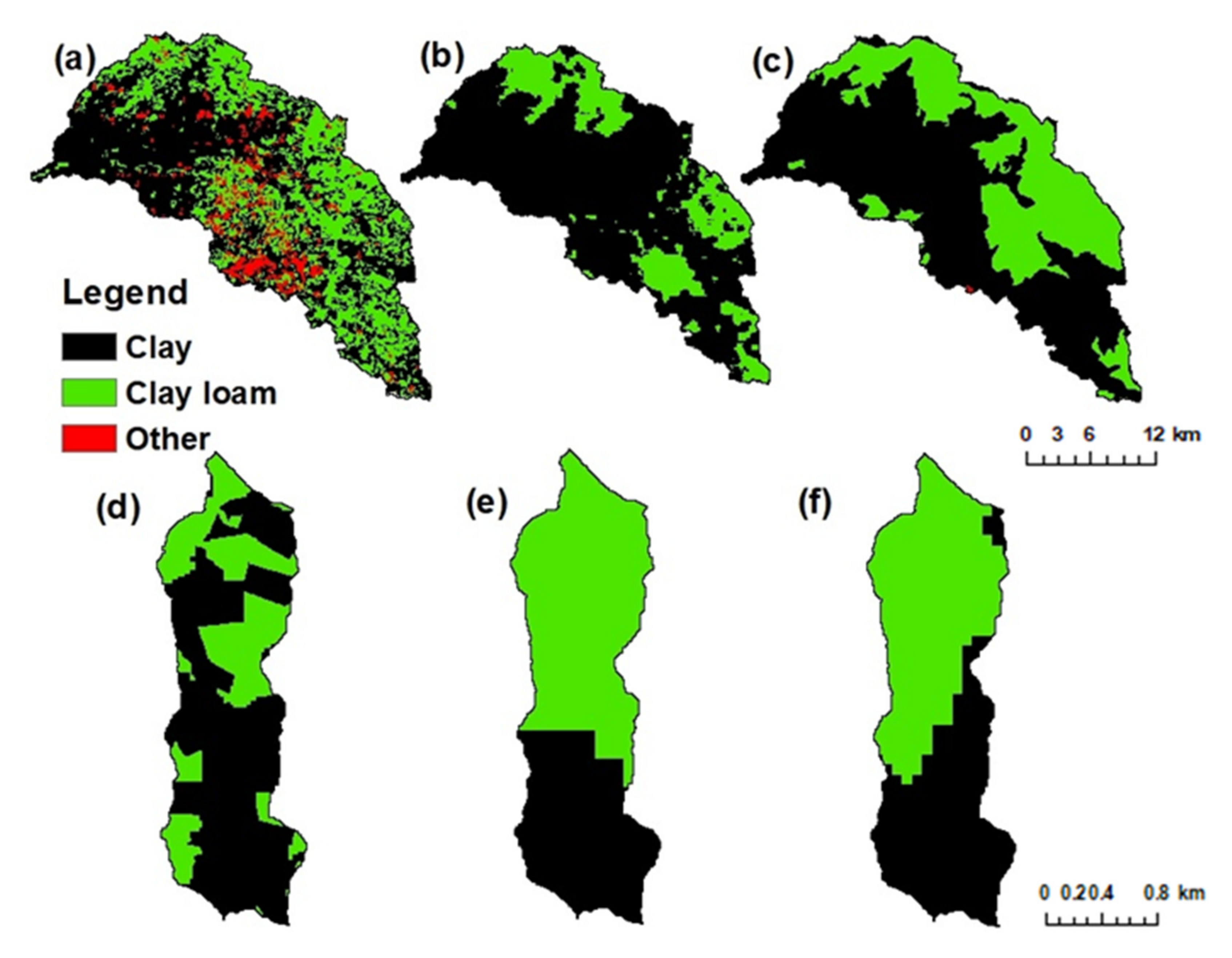
| Rib | ADSWE | 53 | 39 | 8 |
| AfSIS | 76 | 24 | - | |
| FAO | 63.4 | 36.5 | 0.1 | |
| Gomit | ADSWE | 66 | 34 | - |
| AfSIS | 40 | 60 | - | |
| FAO | 45 | 55 | - | |
| Watershed | Soil in-Ventories | Rainfall | Evapotranspiration | Surface Runoff | Baseflow | Recharge to Deep aquifer | Re-evap shal- low Aquifer |
|---|---|---|---|---|---|---|---|
| Rib | ADSWE | 1276 | 466 | 340 | 426 | 20 | 24 |
| AfSIS | 1276 | 525 | 399 | 314 | 14 | 24 | |
| FAO | 1276 | 465 | 401 | 368 | 19 | 24 | |
| Gomit | ADSWE | 988 | 640 | 153 | 128 | 5 | 73 |
| AfSIS | 988 | 836 | 41 | 103 | 0 | 62 | |
| FAO | 988 | 760 | 117 | 60 | 4 | 70 |
| ADSWE | AfSIS | FAO | ||||
|---|---|---|---|---|---|---|
| Rib | Gomit | Rib | Gomit | Rib | Gomit | |
| R2 | 0.83 | 0.70 | 0.85 | 0.72 | 0.83 | 0.6 |
| NSE | −0.77 | −22.5 | −0.41 | −2.7 | −0.73 | -8.5 |
| RVE, % | 125 | 326 | 108 | 110 | 126 | 166 |
| Parameter | Description | Sensitivity Ranking | |||||
|---|---|---|---|---|---|---|---|
| Rib | Gomit | ||||||
| ADSWE | AfSIS | FAO | ADSWE | AfSIS | FAO | ||
| GW_DELAY | Groundwater delay (days) | 1 | 2 | 1 | 9 | 11 | 5 |
| GW_REVAP | Groundwater "revap" coef. | 2 | 3 | 3 | 18 | 16 | 15 |
| CN2 | SCS runoff curve number | 3 | 1 | 2 | 1 | 1 | 1 |
| GWQMN | Threshold depth shallow aquifer for return flow | 4 | 4 | 4 | 12 | 12 | 8 |
| RCHRG_DP | Deep aquif percolation frac | 5 | 5 | 5 | 5 | 10 | 4 |
| ESCO | soil evaporation comp fac. | 6 | 7 | 6 | 2 | 2 | 2 |
| ALPHA_BNK | Baseflow fac. for bank sto. | 7 | 8 | 7 | 7 | 8 | 7 |
| SOL_AWC | Avail. water cap layer | 8 | 11 | 10 | 3 | 3 | 3 |
| ALPH_BF_D | Baseflow fac. deep aquifer | 9 | 10 | 9 | 22 | 22 | 17 |
| CANMX | Maximum canopy storage, | 10 | 6 | 8 | 4 | 5 | 6 |
| SOL_Z | Depth surf. to bottom layer | 18 | 9 | 13 | 11 | 6 | 10 |
| SOL_K | Saturated hydraulic cond. | 19 | 20 | 20 | 10 | 4 | 11 |
| SOL_ALB | Moist soil albedo | 20 | 18 | 17 | 6 | 9 | 9 |
| BIOMIX | Biological mixing eff. | 21 | 22 | 23 | 8 | 7 | 12 |
| Water-shed | Soil Data | Rainfall | Evapo-transpiration | Surface Runoff | Base-Flow | Recharge to Deep Aquifer | Re-evaporation from Shallow Aquifer | |
|---|---|---|---|---|---|---|---|---|
| Rib | PVISSP | ADSWE | 1276 | 537 | 323 | 172 | 0 | 213 |
| AfSIS | 1276 | 606 | 256 | 133 | 134 | 133 | ||
| FAO | 1276 | 534 | 327 | 91 | 159 | 146 | ||
| PVESSP | ADSWE | 1276 | 536 | 318 | 176 | 0 | 215 | |
| AfSIS | 1276 | 595 | 269 | 124 | 137 | 136 | ||
| FAO | 1276 | 529 | 335 | 85 | 135 | 192 | ||
| Gomit | PVISSP | ADSWE | 988 | 840 | 26 | 64 | 19 | 36 |
| AfSIS | 988 | 911 | 6 | 73 | 0 | 0 | ||
| FAO | 988 | 897 | 12 | 40 | 16 | 57 | ||
| PVESSP | ADSWE | 988 | 855 | 11 | 68 | 0 | 52 | |
| AfSIS | 988 | 897 | 5 | 86 | 0 | 0 | ||
| FAO | 988 | 894 | 15 | 40 | 24 | 17 |
| Watershed | Process | Criteria | ADSWE | AfSIS | FAO | |||
|---|---|---|---|---|---|---|---|---|
| PVISSP | PVESSP | PVISSP | PVESSP | PVISSP | PVESSP | |||
| Rib | Calibration | NSE | 0.78 | 0.79 | 0.83 | 0.83 | 0.75 | 0.75 |
| RVE | 7 | 25 | 35 | 35 | 51 | 43 | ||
| Validation | NSE | 0.41 | 0.46 | 0.57 | 0.58 | 0.44 | 0.43 | |
| RVE | 53 | 47 | 54 | 55 | 68 | 69 | ||
| Gomit | Calibration | NSE | 0.63 | 0.60 | 0.59 | 0.46 | 0.67 | 0.67 |
| RVE | 14 | 1 | 12 | 22 | 9 | 1 | ||
© 2020 by the authors. Licensee MDPI, Basel, Switzerland. This article is an open access article distributed under the terms and conditions of the Creative Commons Attribution (CC BY) license (http://creativecommons.org/licenses/by/4.0/).
Share and Cite
Adem, A.A.; Dile, Y.T.; Worqlul, A.W.; Ayana, E.K.; Tilahun, S.A.; Steenhuis, T.S. Assessing Digital Soil Inventories for Predicting Streamflow in the Headwaters of the Blue Nile. Hydrology 2020, 7, 8. https://doi.org/10.3390/hydrology7010008
Adem AA, Dile YT, Worqlul AW, Ayana EK, Tilahun SA, Steenhuis TS. Assessing Digital Soil Inventories for Predicting Streamflow in the Headwaters of the Blue Nile. Hydrology. 2020; 7(1):8. https://doi.org/10.3390/hydrology7010008
Chicago/Turabian StyleAdem, Anwar A., Yihun T. Dile, Abeyou W. Worqlul, Essayas K. Ayana, Seifu A. Tilahun, and Tammo S. Steenhuis. 2020. "Assessing Digital Soil Inventories for Predicting Streamflow in the Headwaters of the Blue Nile" Hydrology 7, no. 1: 8. https://doi.org/10.3390/hydrology7010008
APA StyleAdem, A. A., Dile, Y. T., Worqlul, A. W., Ayana, E. K., Tilahun, S. A., & Steenhuis, T. S. (2020). Assessing Digital Soil Inventories for Predicting Streamflow in the Headwaters of the Blue Nile. Hydrology, 7(1), 8. https://doi.org/10.3390/hydrology7010008