Article

Bottom Sediment Characteristics of a Tropical Lake: Lake Tana, Ethiopia

by
Mebrahtom G. Kebedew
1,2,
Seifu A. Tilahun
1,
Fasikaw A. Zimale
1 and
Tammo S. Steenhuis
1,3,*
1
School of Civil and Water Resources Engineering, Bahir Dar University, Bahir Dar 1000, Ethiopia
2
School of Civil Engineering, Mekelle University, Mekelle 1000, Ethiopia
3
Department of Biological and Environmental Engineering, Cornell University, Ithaca, NY 14850, USA
*
Author to whom correspondence should be addressed.
Hydrology 2020, 7(1), 18; https://doi.org/10.3390/hydrology7010018
Submission received: 20 February 2020 / Revised: 14 March 2020 / Accepted: 16 March 2020 / Published: 19 March 2020

Abstract

:
Sediment concentration of rivers in developing countries has been increasing greatly over the last 50 years due to the conversion of forest to continuously cultivated land with the increasing population. Few studies have addressed its effect on sedimentation and water quality of the lakes by analyzing bottom sediment characteristics. In this study, the objective was to investigate the spatial distribution (and their interrelationships) of the bottom sediment characteristics in the largest lake in Ethiopia, Lake Tana where water hyacinths have been spreading rapidly during the last decade. Sediment samples were collected from the lake bottom at 60 locations and analyzed for texture, organic matter, total nitrogen, and available phosphorus. Bottom sediment samples had a median of 75% clay, 13% silt, and 9% sand. Clay was greatest in the northwestern part and smallest in the areas near the major rivers entering or exiting the lake. Clay percentage and lake depth were strongly correlated. The mean organic matter content of bottom sediment was 16 g kg−1, total nitrogen 0.8 g kg−1, and Olsen available phosphorus 19 mg kg−1. Phosphorus concentrations peaked where water hyacinths were found in the northeastern part of the lake. This study will serve as a baseline for future water quality and sedimentation changes in Lake Tana. In particular, it might aid in explaining the spread of the water hyacinths.

Graphical Abstract

1. Introduction

Lakes are vital in preserving regional environmental and ecological functions and services, such as potable water, irrigation, power generation, fishery, flood contrail, and drought buffer [1]. These functions have been declining especially in the developing world due to rapid population growth that has accelerated land degradation, increasing the amount of sediment and nutrient transported by rivers [2]. Most of the sediment is deposited in floodplains, lakes, and reservoirs [3]. Deposited materials consist of inorganic and organic materials with adsorbed nutrients and contaminants and can threaten the sustainability of lakes [4,5]. The characteristics of suspended and lake bottom sediment composition and associated nutrients depend on the characteristics of the surrounding watershed [6,7], prevailing climate [4,8], and on the residence time [8,9,10,11].
Research on the spatial distribution of bottom sediment characteristics aids in lake management strategies. To do so, previous studies have determined: the spatial distribution pattern to understand sedimentation conditions in Lake Abaya and Chamo, Ethiopia [12] and Kodaikanal and Akkulam-Veli Lake, India [9,10,13]; the source of the organic matter deposition in Lake Victoria [14], Lake Kodaikanal, Manasbal, Wular, and Anchar lakes, India [15,16]; distribution of total phosphorus in Southern Green Bay of Lake Michigan [17], the release of nutrients from the bottom sediments in the water column for Lake Rotoiti in New Zealand [18] and Poyang Lake in China [19]; and the overall implication on lake sustainability of Minnesota lakes, USA [20].
In this study, the current lake bottom sediment characteristics of Lake Tana were investigated. The total sediment layer in Lake Tana accumulated over a 250,000 year period is greater than 100 m [21,22]. Less than 100 years ago, Lake Tana was described as a pristine lake with a sandy bottom at the inlets [23]. In the 1960s, with the increasing population pressure, sedimentation of the lake increased greatly over historic rates and river deltas formed [24]. The water quality of the lake declined as well [25] with the increased sediment-associated and dissolved nutrient inputs [26]. This has resulted in poor light penetration [27], declined fish production [28], and increased water hyacinth acreage from 20 ha in 2012 to over 30,000 ha or 10% of the lake area in 2018 [29].
Most of the previous research on Lake Tana focused on pollution [30], eutrophication [31], water hyacinth coverage and potential infestations [29,32], the effect of nutrient availability and water transparency on primary production [25], location dynamics of the major phytoplankton and zooplankton communities [33], ecohydrological status, fisheries and fish evaluation biology [34] sediment physicochemical characteristics [35], and the status of water quality [36]. Several bathymetries surveys were conducted indicating sedimentation rates of 12 Tg yr−1 to 108 Tg yr−1 [37]. Finally, sediment budget calculations showed that a major portion of the sediment was deposited in the river floodplains [38,39].
Despite these studies, little is known about the lake bottom sediment characteristics and nutrient content. The only recent study available [35] reports on the nutrient sediment content of 20 samples taken near the lakeshore with aquatic vegetation. Studies on sediment characteristics are not available. The objective is therefore, to investigate the spatial distribution (and their inter relationships) of the bottom sediment characteristics throughout Lake Tana. The texture and the organic matter, total nitrogen and available phosphorus content of the bottom sediments, and the lake depth were measured in approximately a 10 km by 10 km grid with additional measurements taken close to the shoreline.

2. Materials and Methods
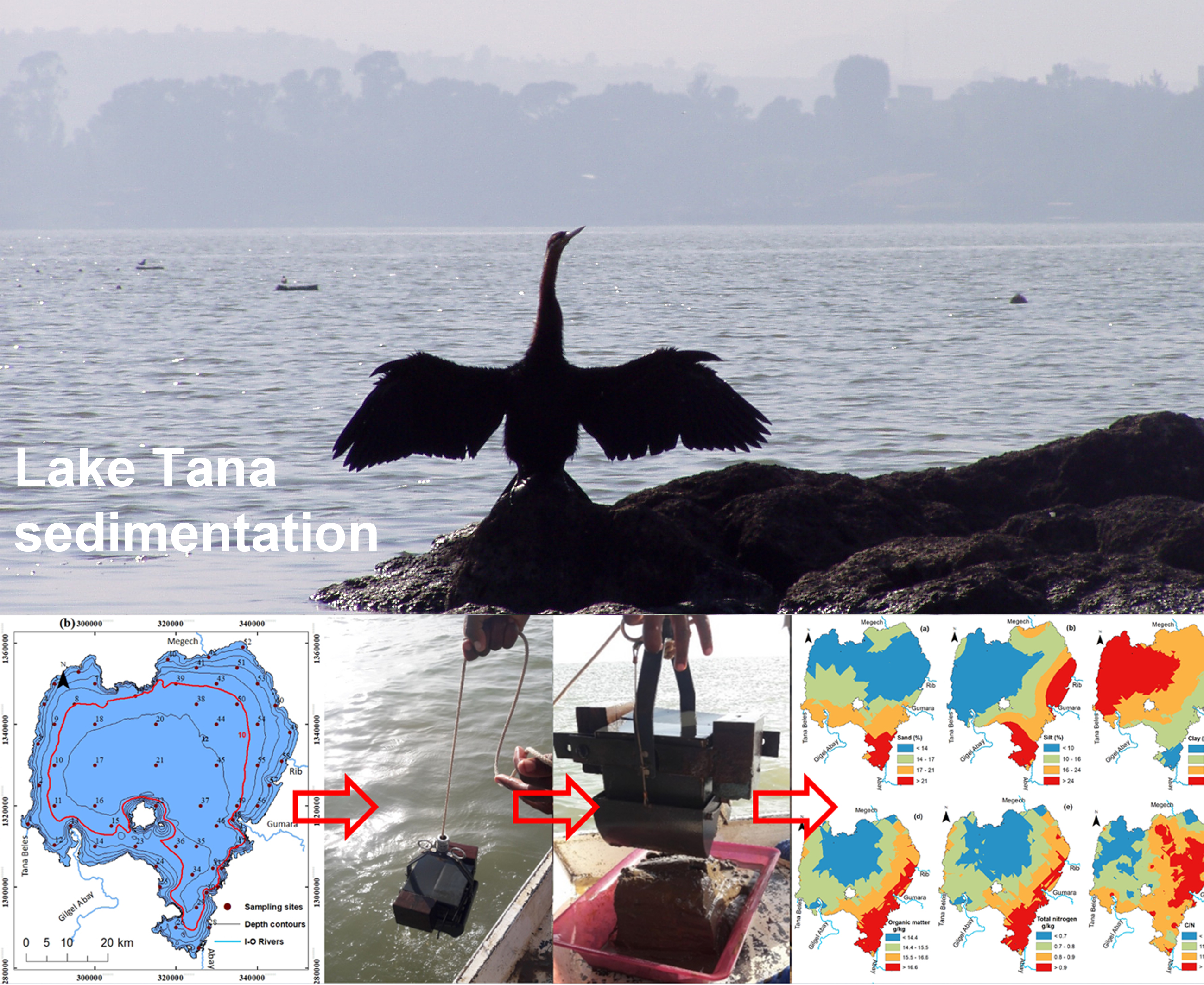
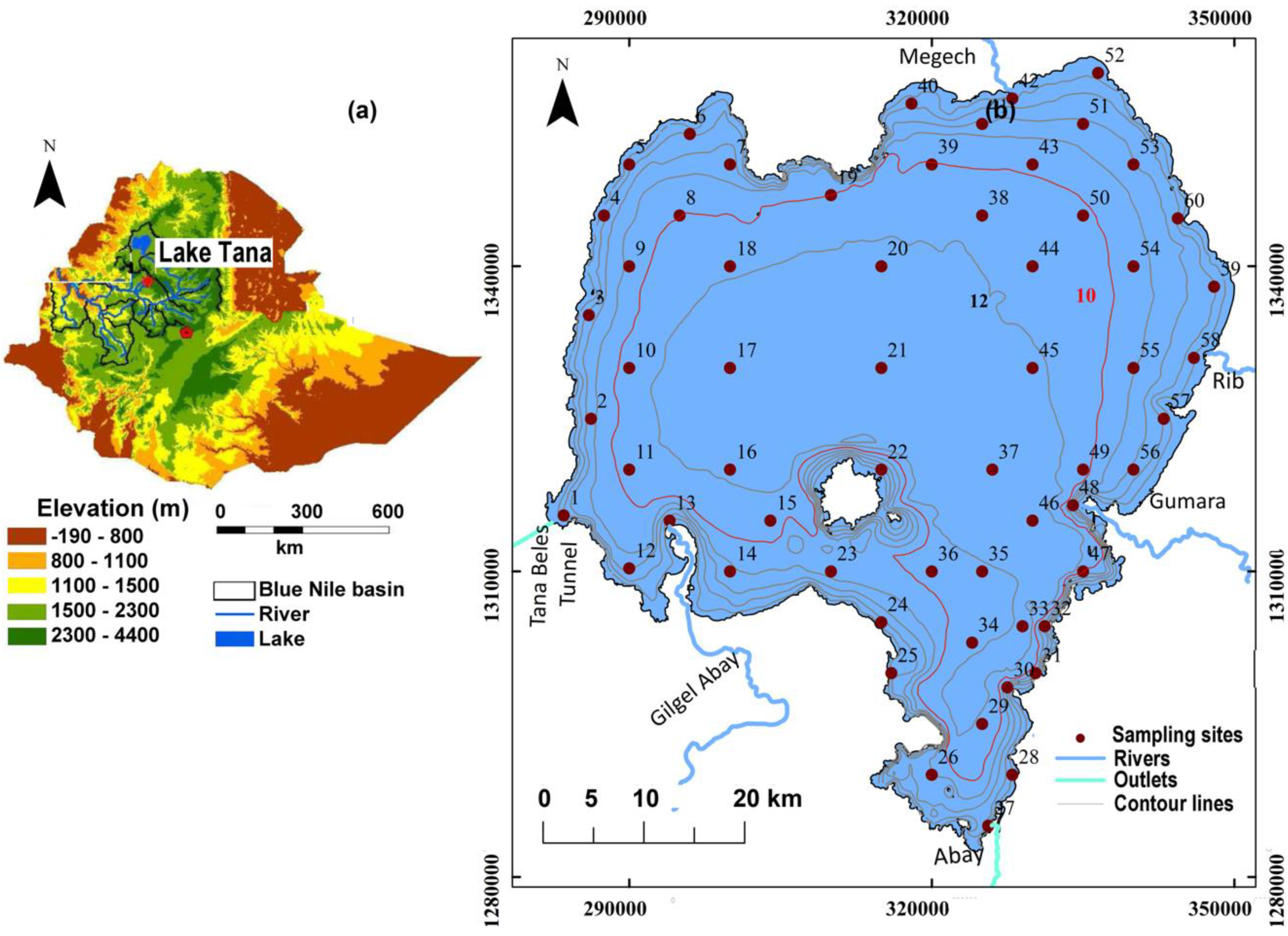
2.1. Study Area

Lake Tana, located in the headwaters of the Blue Nile in the north-western Ethiopian highlands, is the largest lake in Ethiopia (Figure 1) [27]. The average depth is 9 m, and the area is 3041 km2 [40]. It serves as a natural reservoir for Tis Abay and Tana Beles hydropower stations. It is an important source of income for the local communities [41]. The lake water is used for irrigation, hydropower, fishing, transportation, and tourism [42]. Lake Tana and surrounding areas were designated by the government as a growth corridor with several irrigation schemes [43].
The lake is fed by more than 40 seasonal rivers and 4 permanent rivers: Gilgel Abay from the south, Megech from the north, and Gumara and Rib from the east. The major rivers contribute about 80% of the total annual inflow and 62% of the sediment load to the lake [39,44]. The sediment concentrations in the rivers have been increasing in the past fifty years [24]. Sediment concentrations of more than 10 g L−1 are not uncommon from watersheds with active gully erosion [45]. In addition, the nutrient input from the upland agricultural areas has increased [26,46]. Phosphorus concentrations in the lake water have been rising [47] and have resulted in a progressive change of the lake from mesotrophic to eutrophic status [31].

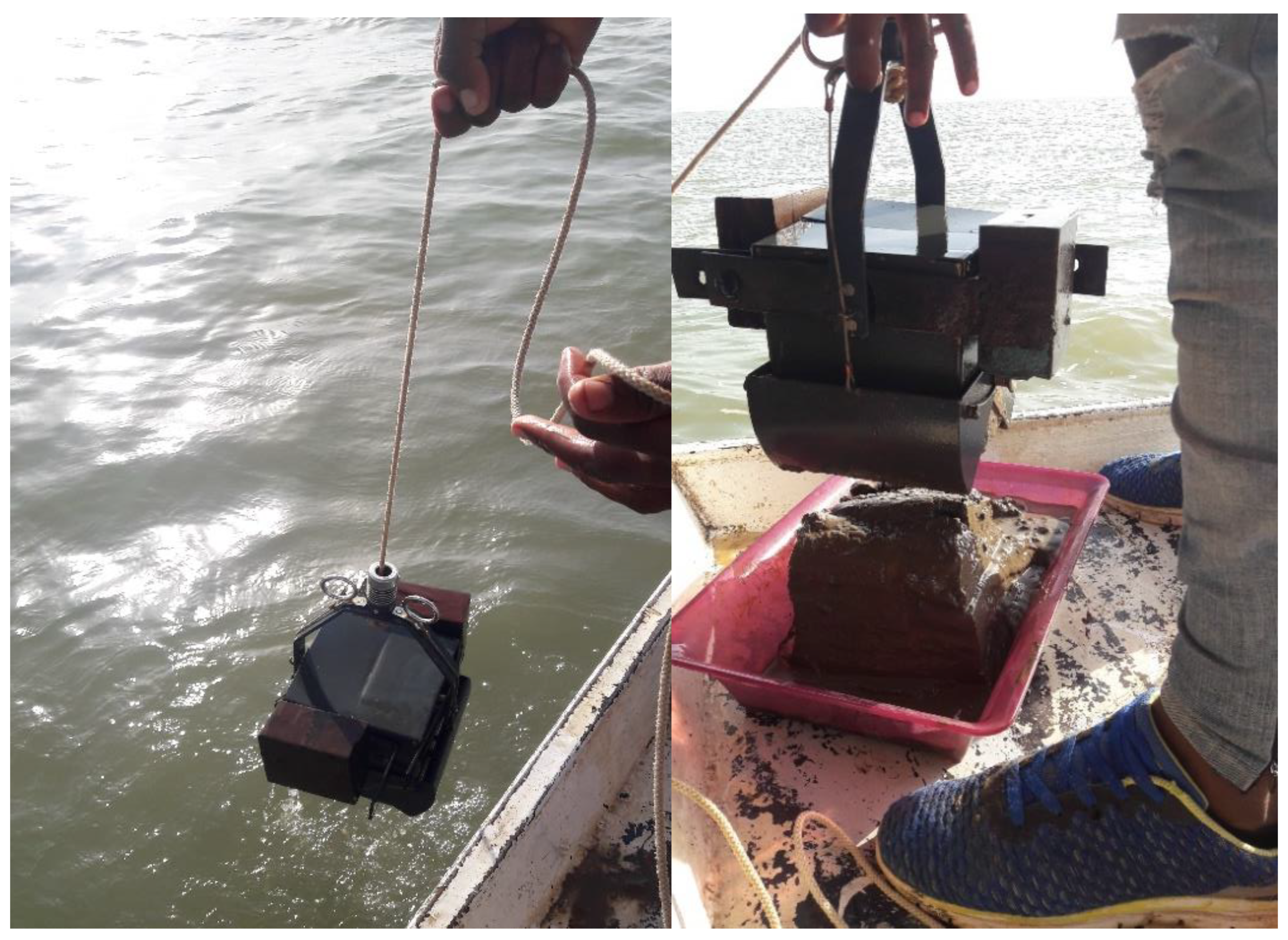
2.2. Bottom Sediment Sampling

From 27 February to 6 March 2018, sediment samples were collected from deposited sediments at the bottom of Lake Tana. In the main part of the lake at a depth greater than 10 m depth where the sedimentation was uniform, samples were taken in a grid of approximately 10 km by 10 km (Figure 1 shows the 10 m contour line). At depths less than 10 m in the nearshore areas, additional bottom sediment samples were taken at locations where sediment composition was expected to change rapidly (Figure 1). A total of 60 sediment samples were collected The GPS locations of all sampling locations were used for navigation. The standard Ekman grab sampler [48] was used to collect bottom sediment samplers. For sampling at a depth greater than 6 m, a weight of 8 kg was attached to the sampler (Figure 2 shows the configuration). The minimum weight of the sediment sample collected was 1 kg, which was a wet weight. In cases where a greater sample was collected; a subsample was taken from 1 to 1.5 kg. After collection, samples were labeled and stored in a sealed bag for further analysis (Table A1 in the Appendix).

2.3. Analytical Methods

Collected bottom sediment samples were analyzed in Amhara Design and Supervision Works Enterprise, Soil Chemistry Laboratory. Sediment samples were air-dried, ground, and passed through a 2 mm sieve. The hydrometer method was used for determining the sand, silt, and clay fractions [49]. The textural classification was based on USDA soil classification criteria [50]. Organic matter content was determined with the Walkley Black rapid titration method, total nitrogen with Kjeldahl’s method, and available phosphorus with the Olsen method [51]. The organic carbon content was derived assuming that 58% of organic matter is organic carbon [52].

2.4. Interpolation

The analytical data for the 60 bottom sediment sampling points were entered in Excel and then imported into Geospatial Analyst Tool extension, ArcGIS (version 10.4.1), for interpolation. The ordinary kriging, geostatistical interpolation, with an exponential semi-variogram method was used to find the spatial distribution of bottom sediment texture, organic matter, total nitrogen, C/N, and available phosphorus of the lake. Unlike the deterministic method, ordinary kriging uses autocorrelation or statistical relationships among a group of measured points to create surfaces [53]. A best fit exponential semi-variogram is fitted to the empirical semi-variogram that depicts the spatial autocorrelation of the measured points. The fitted semi-variogram will further be used to predict the unknown points within the measured values for spatial interpolation.

2.5. Statistical Methods

Microsoft Excel 2019 was used to calculate the descriptive statistics, box plots, and to perform regression analysis with lake depth on the bottom sediments. The relationship between measured sediment parameters was evaluated with Pearson’s correlation matrix.

3. Results

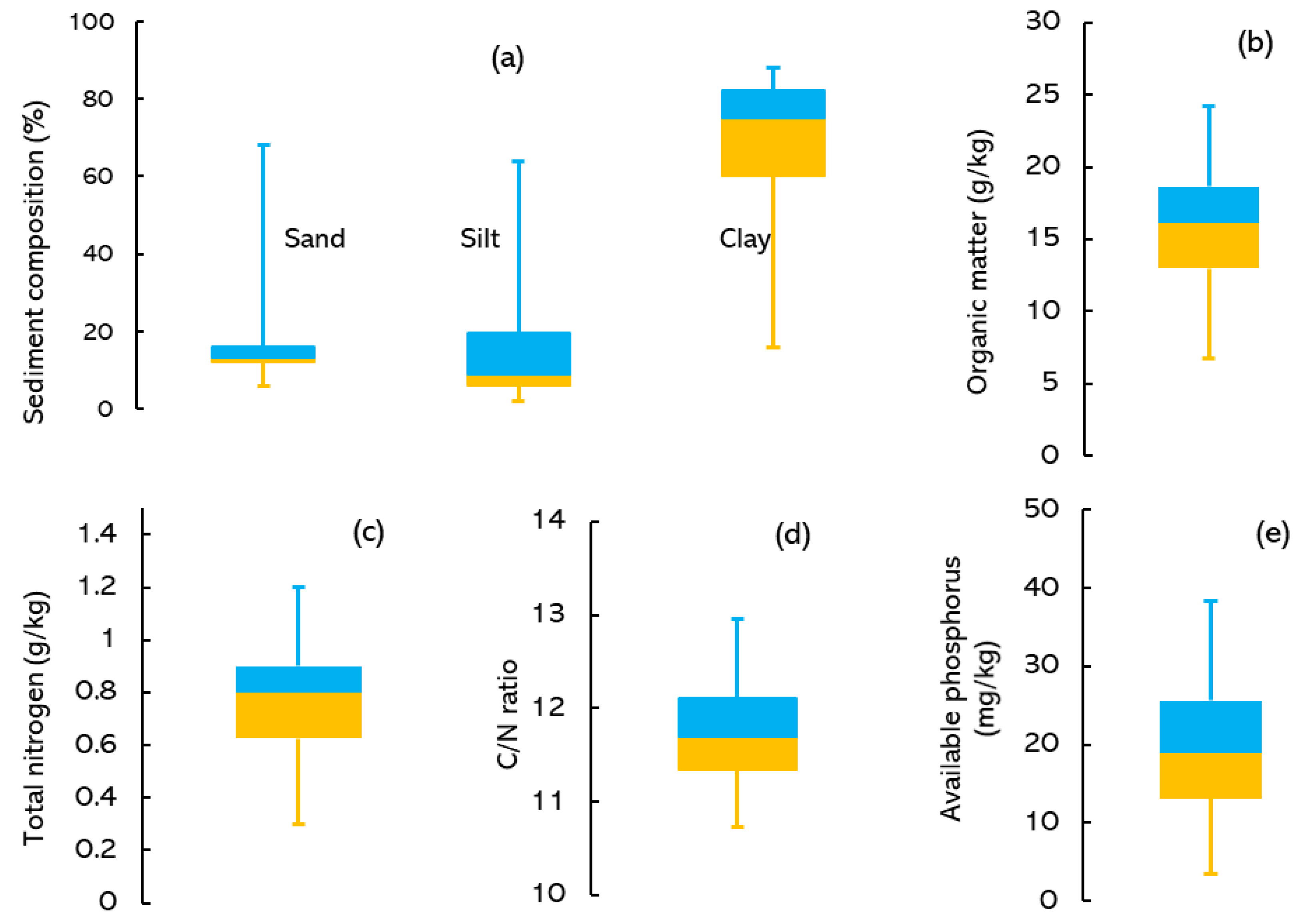
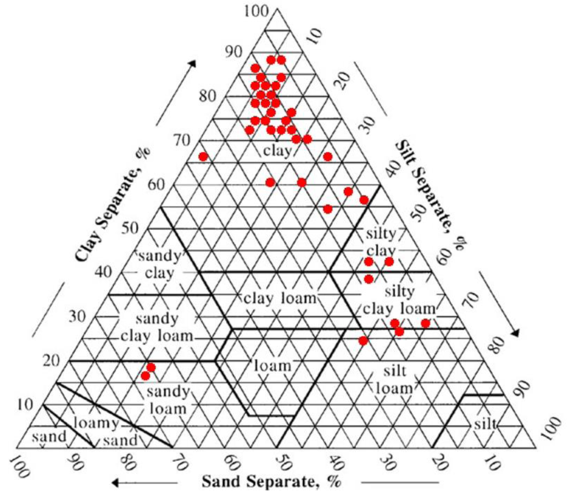
3.1. Bottom Sediment Characteristics of Lake Tana

The bottom sediment had an average of 16% sand, 17% silt, and 67% clay. The median is 13% sand, 9% silt, and 75% for clay (Table A1 in the Appendix). The clay content was positively skewed with lower outliers, and sand and silt fractions were negatively skewed with upper outliers (Figure 3, Table S1 in the Supplemental Material). Based on USDA soil classification, the bottom sediment composition, texture class, was mainly clay with limited occurrence of sandy loams at sampling points 13, 27, and 31, silty loams at sampling points 1 (Tana Beles tunnel inlet) and 25, silty clay loam at sampling points 58, 24, and 28, and silty clay at sampling points 56 and 57 (Figure 4; locations of the sampling points are given in Figure 1).
The average organic matter content of the sediment was 16 g kg−1 with a range of 7 to 24g kg−1, total nitrogen was from 0.3 to 1.2 g kg−1 with an average value of 0.8 g kg−1, and the sediment available phosphorus was 19 mg kg−1 and ranged between 3.5 to 39 mg kg−1 (Table A1). The organic matter was with lower outliers, total nitrogen was normally distributed, and available phosphorus and the C/N ratio were positively skewed (Table S1 in the Supplemental Material). However, the medians are fairly close to the center of the box, and the whiskers are of approximately equal length for the contents of organic matter, total nitrogen, C/N, and available phosphorus (Figure 3).

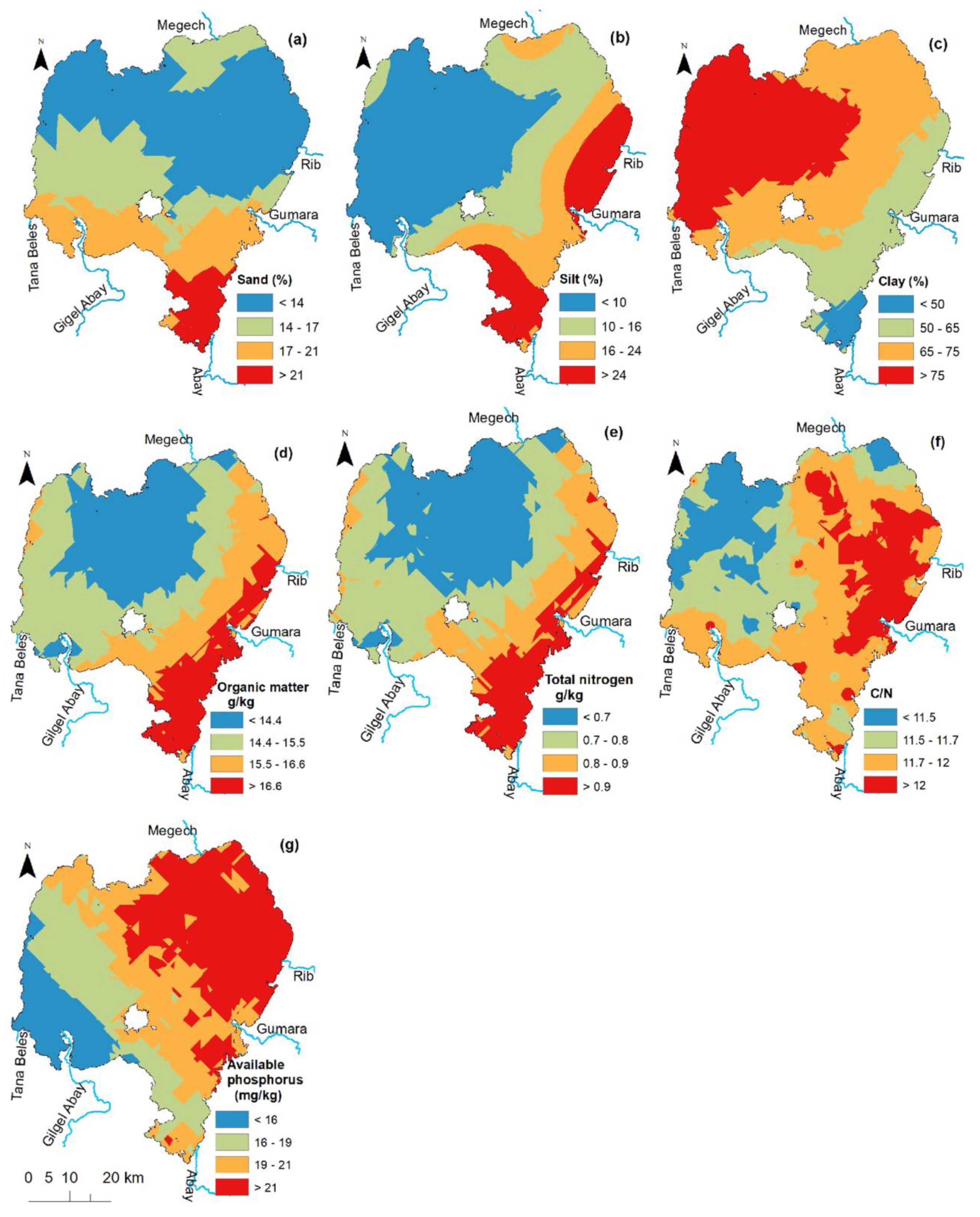
3.2. Spatial Distribution

Based on the 60 bottom sediment samples, maps were created using ordinary kriging with an exponential semi-variogram (Figure S1 in the Supplemental Material) of the contents of sand, silt, and clay (Figure 5a–c), the concentrations of organic matter, total N and available P (Figure 5d–f), and the C/N ratio, which has the lowest RMSE value. The sediment composition data (Figure 3) had a large skew and were log-transformed to make the distribution normal. The other parameters were normally distributed.
The semi-variograms depicted in Figure S1 show there was a large nugget effect for all measured parameters indicating that the variation at a distance smaller than approximately 10 km was large compared to the sill or the maximum variability between two points. In the case of the organic matter, total N, and available phosphorus (Figure S1d–f), the nugget effect and the sill are almost equal, indicating that the large- and small-scale variability are nearly equal. The clay percentage (Figure S1c) is the only parameter that shows a good spatial dependence with an effective range (defined as lag at which 95% of the sill is exceeded) of 50–60 km.
The kriged maps in Figure 5 show that the sand and silt fractions were the greatest near the outlet of the lake (Figure 5a,b) where the Blue Nile starts. One sampling point (13) near the Gilgel Abay had the greatest sand content (68%, Table A1). Silt content was also elevated near Rib and Gumara rivers on the east side of the lake (station 48) and Rib inlet (station 58). The largest amount of clay content was found at the northwestern and deeper parts of the lake (Figure 5c). More than 42% of the lakebed had more than 75% clay, and only 3% of the lake had less than 50% clay.
The spatial distribution of the organic matter, (including organic carbon), and total nitrogen in the bottom sediments was similar. The minimum concentrations were observed in the central and the northern parts and the maximum in the southern and eastern sides of the lake (Figure 5d–f). Organic matter content greater than 20 g kg−1 was observed at sampling points 41 near Megech inlet, 58, 47, 44, 59, 60, and 57 near Rib inlet and nearby areas, and 28 and 32 in the southeastern part (Figure 5d; Table A1; Figure 1 gives the locations of the sampling stations). The largest C/N ratios were observed in the southeastern part of the lake near the Gumara and Rib rivers. The southwestern part had relatively more carbon than nitrogen (Figure 5e). Available phosphorus increased from the western part near the Gilgel Abay River inlet to the northeast in an area that stretches for Megech and Rib rivers (Figure 5g). The latter was the location where the water hyacinths are most prominent.

3.3. Correlation

The analysis showed a very strong positive correlation between the contents of organic matter and total nitrogen and a strong correlation between clay content and lake depth. A weak correlation between silt content and organic matter and silt content and total nitrogen was found. A strong negative correlation occurred between silt and clay content and between silt content and lake depth. A moderate negative correlation was observed between sand and clay content. However, the linear correlation of available phosphorus with the other parameters was very weak. In addition, the linear correlation sand fraction with all measured parameters except clay content was very weak.

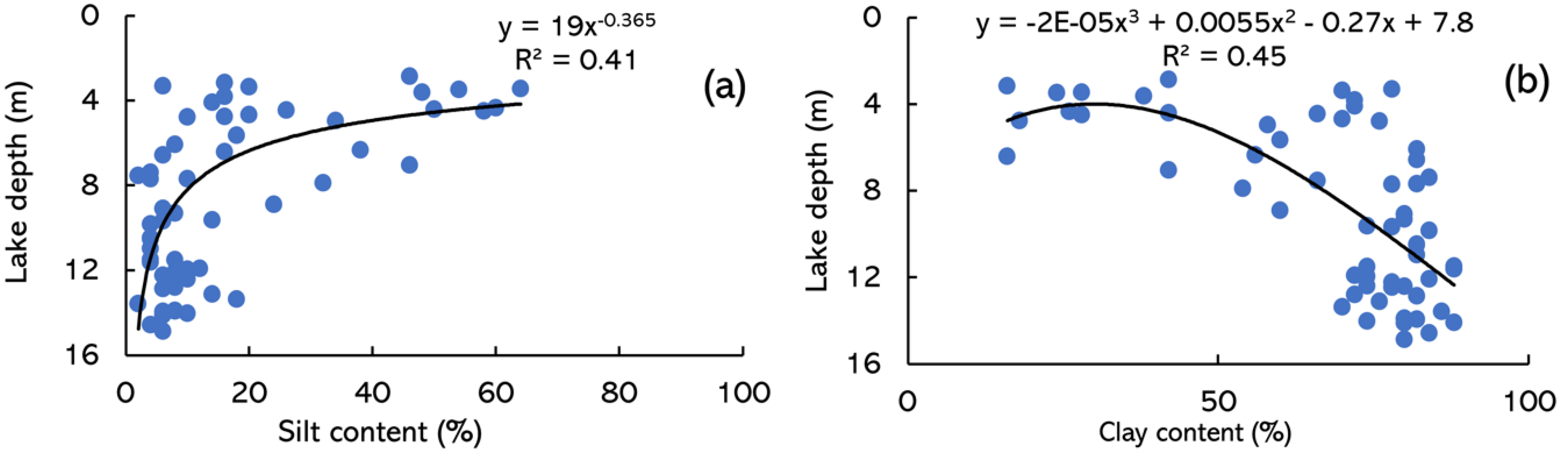
3.4. Relationship with Lake Depth

The results of regression plots (Figure 6a,b) confirm the results in Table 1 that with increasing lake depth, the clay content increased, and the silt content decreased. All other measured parameters were not related to lake depth, although in some cases a weak trend could be detected (Figure S2 in the Supplemental Material).

4. Discussion

The bottom sediments of Lake Tana were sampled on a grid of approximately 10 by 10 km (Figure 1). The 60-sediment sample had a median of 75% clay, 9% silt, and 13% sand (Figure 3; Table A1). Averages due to the skewness of the textural composition (Figure 3) are lower flow clay with 65% and slightly greater for both silt (17%) and sand (16%). The sediments in the deepest part of the lake had the greatest percentage clay and were classified according to the USDA classification as clay (Figure 4). Sandy deposits were found near the inlet of the major rivers and outlet to the Blue Nile (Figure 5). The sand concentration near the major rivers is greater, especially near the Gilgel Abay, which does not have a substantial floodplain, because sand drops out first due to its fast settling velocity [54]. The rapid growth of the peninsulas of Gilgel Abay [40] and Gumara [55] are also a result of this process. The high sand content near the exit of the Blue Nile is caused by a different process and originates from the sediments resuspended by the wind; the suspended fine particles are transported away in the Blue Nile river water, leaving the sand particles behind [56].
In comparing the bottom sediments of Lake Tana, we find that the bottom sediment samples from the northern part of the 223,000 km2 Lake Victoria (Uganda and Kenya) have a slightly lower clay percentage of 61%, more silt 35%, and less sand (4%) [57]. The textural classification of the 947 samples from Lake Abaya and Chamo in the southern part of Ethiopia is mainly silty clay, indicating less clay and more silt than Lake Tana. The depth of these two lakes is approximately the same, but the surface area is only one-third of Lake Tana [12]. The small tropical Lake Berijam in India of 0.24 km2 consists of silty and sandy clays [15].
The bottom sediments of, the on average over 300 m deep and 33,000 km2 large, Lake Tanganyika and the 270 m deep and 30,000 km2 Lake Malawi in the Rift Valley are much sandier than Lake Tana [58,59,60]. The sediments near the inlets of the rivers have more clay than the rest of Lake Malawi due to the deposition of eroded material from agricultural fields [58,60]. Another tropical lake with a sandier bottom than Lake Tana is the 9 m deep and 160 km2 large Lake Navashi in Kenya that has 33% clay, 40% silt, and 30% sand [61]. The inflow and outflow to this lake that is located in the Rift valley was mostly via the subsurface. Finally, the bottom sediment of the small tropical Kadaikanal Lake India was sand.
The organic matter content in this study with an average of 16 g kg−1 (Figure 3b, Table A1) was greater than that of the limited data collected 20 years ago [62] but less than the study conducted 5 years ago that sampled the lake near the shoreline [35] that was dominated by aquatic plants [36]. The organic matter content on Lake Tana was small compared with Lake Abaya and Chamo [12] in Ethiopia, Lake Victoria [14] in Central Africa, and the Waler and Berijam lakes in India [19,63]. The low organic matter and total N content in Lake Tana is a consequence of agricultural land in the watershed that is low in organic matter and the shallow depth. Because of the shallow depth, the lake is well-mixed and fully oxidized, enhancing mineralization [16]. The lowest percentage of organic matter in the western and deeper areas indicates that the mineralization in the deepest part of the lake is enhanced [64]. The southern part is also influenced by the urbanized areas and aquatic plants.
The C/N ratio varied from 10.5 to 13 and was greater on the east side of the lake than the west site (Figure 3 and Figure 5). The source of organic matter in the sediment of Lake Tana was from both aquatic and terrestrial origins because algae have a C/N ratio of less than 10 and terrestrial inputs have a C/N ratio greater than 20 [65]. In the deeper parts on the west side of the lake farthest away from the main rivers with the C/N ratios closest to 10, there is mainly aquatic organic matter, while in the western part, some terrestrial organic matter is mixed in.
The available phosphorus in the sediment ranged from 4 mg to 31 mg kg−1. The greatest concentrations were found in the northeast part of the lake. This was also the location where the water hyacinths were found [29,32]. The available phosphorus concentrations in the lake bottom sediments were not related to any other measured parameter (Table 1), indicating that the conversion processes that caused the pattern are unique. We should note that Gumara and Rib rivers that enter the lake on the east side have during the rainy season a dissolved P concentration that exceeds the lake concentration [27,30,47,66]. In the Awramba watershed close to lake outlet, the concentration was about three to four times the observed average dissolved phosphorus content in the lake of 0.18 mg L−1 [26,66]. This excess dissolved P concentration will adsorb on the lake sediment until a new equilibrium is established, thereby increasing the sediment phosphorus concentration. However, it is not obvious why this increase in bottom concentration is the greatest in the northeast side of the lake. A planned study on lake circulation might provide the answer.

5. Conclusions

Sixty sediment samples were collected from the bottom of Lake Tana. Textural analysis of the samples showed that the sediment was mainly clay. Spatially, silt and sand fractions were mixed in with the clay near the inlet of the four major rivers and Blue Nile outlet. Clay content was strongly related with lake depth and silt content was negatively correlated. The average organic matter content of the bottom sediment was 16 g kg−1, total nitrogen 0.8 g kg−1, and available phosphorous 19 mg kg−1 and were not correlated significantly with lake depth. Available phosphorus that was not correlated with any of the measured parameters was the greatest in the shallow northeastern part of the lake that was invaded by water hyacinths. Future studies will address the spatial distribution the bottom sediment with suspended sediment and dissolved nutrients in the river and lake water circulation including water hyacinth invasion.

Supplementary Materials

The following are available online at https://www.mdpi.com/2306-5338/7/1/18/s1, Table S1, Descriptive statistics of Lake Tana bottom sediment composition and sediment nutrients: organic matter, organic carbon, total nitrogen, C/N ratio, and available phosphorus fractions. Figure S1, Kriging variogram model for spatial distribution of Lake Tana bottom sediment characteristics: (a) sand fraction, (b) silt fraction, (c) clay fraction, (d) organic matter fraction, (e) sediment total nitrogen, (f) sediment available phosphorus, and (g) carbon to nitrogen ratio on Lake Tana bottom sediments. Figure S1, bottom sediment characteristics of Lake Tana: (a) sand content with lake depth, (b) organic matter content with lake depth, (c) sediment total nitrogen content with lake depth, (d) C/N ratio with lake depth, and (e) sediment available phosphorous content with lake depth.

Author Contributions

M.G.K. contributed during conceptualization, data collection, data analysis, writing the original draft manuscript, and improving the manuscript based on the comments and suggestions of the coauthors. S.A.T. contributed in shaping the objective, methods, project administration, supervision, review, and editing. F.A.Z. helped in conceptualizing the study and providing comments and suggestions. T.S.S. contributed during conceptualization, overall content, structure and English of the paper, improving the English, and supervising. All authors have read and agreed to the published version of the manuscript.

Funding

The research was funded by the EXCEED–SWINDON project “Excellence Center for Development Cooperation–Sustainable Water Management in developing countries” centered at Technical University of Braunschweig, Germany and Blue Nile Water Institute of Bahir Dar University Ethiopia. Additional funding was provided by the Robert S. McNamara Fellowships Program (World Bank), and an anonymous gift made to Cornell.

Acknowledgments

We acknowledge the dedication of Bantesew Muluye and Getahun Birara during sampling of the bottom sediment of Lake Tana. They also shared willingly in the dangers of sampling of the 3000 km2 Lake Tana in a small boat.

Conflicts of Interest

The authors declare that they do not have a conflict of interest.

Appendix A

Table A1. Bottom sediment characteristics (texture, organic matter (OM), total nitrogen (TN), available phosphorus (AV.P), organic carbon (OC), C/N ratio, lake depth (Dept.), and texture class).
Sit. No XY Sand (%)Clay (%)Silt (%)OM g kg−1TN g kg−1OC g kg−1C/N Av. P mg kg−1Dept. (m)Texture Class
128300013150001082812.10.6711.79.56.1Silty loam
2286200132500012781013.40.77.811.115.47.7Heavy clay
3286000133520014761018.20.910.611.78.64.8Heavy clay
4287500134500010702019.51.011.311.3124.7Heavy clay
5290000135000010702014.80.78.612.3123.4Heavy clay
629600013530001678617.50.910.211.36.93.3Heavy clay
730000013500001482411.40.66.61117.17.7Heavy clay
829500013450001482416.10.89.311.722.310.5Heavy clay
929000013400001678617.50.910.211.327.49.7Heavy clay
102900001330000888414.10.78.211.710.311.6Heavy clay
112900001320000888416.10.89.311.77.811.5Heavy clay
1229000013103001282616.10.89.311.721.46.6Heavy clay
13294000131500068161610.80.56.312.58.63.2Sandy loam
1430000013100001480620.21.011.711.77.89.1Heavy clay
153040001315000167869.40.55.510.914.612.2Heavy clay
1630000013200001286216.10.89.311.78.613.6Heavy clay
173000001330000688613.40.77.811.118.914.1Heavy clay
183350001354000128449.40.55.510.925.77.5Heavy clay
193100001347000148247.40.44.310.725.711Heavy clay
203150001340000128088.10.44.711.734.213.9Heavy clay
2131500013300001480610.80.56.312.525.714.9Heavy clay
2231500013200001280813.40.77.811.120.613.9Heavy clay
23310000131000012741418.20.910.611.718.99.6Heavy clay
24315000130500014285810.80.56.312.59.54.5Silty clay loam
25316000130000014266024.20.121411.718.94.4Silty loam
26320000129000016602418.20.910.611.7188.9Clay
27325600128500066181614.80.78.612.313.74.8Sandy loam
28328000129000014384823.51.213.611.412.93.6Silty clay loam
2932500012950001478817.50.910.211.327.412.5Heavy clay
303275001298600656388.70.4512.638.56.3Clay
31330300130000068161616.10.89.311.7186.4Sandy loam
32331200130460022601822.91.113.312.117.15.7Clay
33329000130460016741014.10.78.211.76.114Heavy clay
34324000130300016741019.51.011.311.328.212.4Heavy clay
3532500013100002072818.80.910.912.116.312.8Heavy clay
36320000131000016741018.20.910.611.724.812Heavy clay
3732600013200001480616.10.89.311.72414.1Heavy clay
3832500013450001280818.80.910.912.16.912.4Heavy clay
393200001350000187486.70.33.91317.111.5Heavy clay
40318000135600014721414.10.78.211.731.64.1Heavy clay
41325000135400014543220.21.011.711.714.67.9Clay
42328000135650012424616.10.89.311.714.62.9Clay
4333000013500001482416.10.89.311.727.410.5Heavy clay
4433000013400001282621.51.112.511.332.512.9Heavy clay
45330000133000012701812.10.6711.723.113.4Heavy clay
4633000013150001282614.80.78.612.320.613.9Heavy clay
47335000131000016721223.51.213.611.432.511.9Heavy clay
48334000131650022245416.80.89.712.223.13.5Clay loam
49335000132000010761410.80.56.312.513.713.1Heavy clay
4934800013380008583422.21.112.911.729.15Clay
503350001345000884814.80.78.612.319.712.1Heavy clay
5130000013400003266217.50.910.211.330.812.8Heavy clay
52336500135900012721613.40.77.811.1243.8Heavy clay
5334000013500001284414.10.78.211.718.97.4Heavy clay
5434000013400001284410.80.56.312.525.79.8Heavy clay
5534000013300001280812.80.67.412.43.59.3Heavy clay
56340000132000012424616.80.89.712.226.57.1Clay
5734300013250008425021.51.112.511.3184.4Clay
5834600013310008286420.21.011.711.729.93.4Silty clay loam
5934800013380008583422.21.112.911.729.14.951Clay
6034440013447008662620.21.011.711.727.44.5Heavy clay

References

  1. Hou, X.; Feng, L.; Duan, H.; Chen, X.; Sun, D.; Shi, K. Fifteen-year monitoring of the turbidity dynamics in large lakes and reservoirs in the middle and lower basin of the yangtze river, China. Remote Sens. Environ. 2017, 190, 107–121. [Google Scholar] [CrossRef]
  2. Mortimore, M. Population growth and land degradation. GeoJournal 1993, 31, 15–21. [Google Scholar] [CrossRef]
  3. Kim, S.M.; Jang, T.I.; Kang, M.S.; Im, S.J.; Park, S.W. Gis-based lake sediment budget estimation taking into consideration land use change in an urbanizing catchment area. Environ. Earth Sci. 2014, 71, 2155–2165. [Google Scholar] [CrossRef]
  4. Chapman, D.V. Water Quality Assessments: A Guide to the Use of Biota, Sediments, and Water in Environmental Monitoring; World Health Organization: Geneva, Switzerland, 1996. [Google Scholar]
  5. Almada Rojas, G.; Palafox, J.T.P.; Uribe, D.M.; Gaytan, J.M.; Garcia, L.F.C.; Figueroa, J.L.A. Morphological, sediment and soil chemical characteristics of dry tropical shallow reservoirs in the southern mexican heghlands. J. Limnol. 2011, 70, 139. [Google Scholar] [CrossRef]
  6. Morris, G.L.; Fan, J. Reservoir Sedimentation Handbook: Design and Management of Dams, Reservoirs, and Watersheds for Sustainable Use; McGraw Hill Professional: New York, NY, USA, 1998. [Google Scholar]
  7. Danz, N.P.; Niemi, G.J.; Regal, R.R.; Hollenhorst, T.; Johnson, L.B.; Hanowski, J.M.; Axler, R.P.; Ciborowski, J.J.; Hrabik, T.; Brady, V.J. Integrated measures of anthropogenic stress in the us great lakes basin. Environ. Manag. 2007, 39, 631–647. [Google Scholar] [CrossRef]
  8. Håkanson, L.; Jansson, M. Principles of Lake Sedimentology; Springer: Berlin/Heidelberg, Germany, 1983; Volume 316. [Google Scholar]
  9. Balamurugan, P.; Vasudevan, S.; Selvaganapathi, R.; Nishikanth, C. Spatial distribution of grain size characteristics and its role in interpreting the sedimentary depositional environment, Kodaikanal Lake, Tamil Nadu, India. J. Earth Sci. Clim. Chang. 2014, 5, 2. [Google Scholar]
  10. Mclaren, P.; Bowles, D. The effects of sediment transport on grain-size distributions. J. Sediment. Petrol. 1985, 55, 457–470. [Google Scholar]
  11. Shu, G.; Collins, M. The use of grain size trends in marine sediment dynamics: A review. Chin. J. Oceanol. Limnol. 2001, 19, 265–271. [Google Scholar] [CrossRef]
  12. Gebremariam, B. Basin Scale Sedimentary and Water Quality: Responses to External Forcing in Lake Abaya, Southern Ethiopian Rift Valley. 2009. Available online: https://refubium.fu-berlin.de/handle/fub188/6983 (accessed on 19 March 2019).
  13. Shah, R.A.; Achyuthan, H.; Puthan-Veettil, R.S.; Derwaish, U.; Rafiq, M. Sediment distribution pattern and environmental implications of physico-chemical characteristics of the Akkulam-Veli Lake, South India. Appl. Water Sci. 2019, 9, 188. [Google Scholar] [CrossRef] [Green Version]
  14. Mwamburi, J. Spatial variations in sedimentary organic matter in surficial lake sediments of nyanza gulf (lake victoria, kenya) after invasion of water hyacinth. Lakes Reserv. Res. Manag. 2016, 21, 94–113. [Google Scholar] [CrossRef]
  15. Vijayaraj, R.; Achyuthan, H. Distribution of sediments and organic matter source: Berijam lake, tamil nadu. J. Geol. Soc. India 2015, 86, 620–626. [Google Scholar] [CrossRef]
  16. Lone, A.M.; Shah, R.A.; Achyuthan, H.; Rafiq, M. Source identification of organic matter using c/n ratio in freshwater lakes of Kashmir Valley, Western Himalaya, India. Himal. Geol. 2018, 39, 101–114. [Google Scholar]
  17. Hamidi, S.A.; Hosseiny, H.; Ekhtari, N.; Khazaei, B. Using modis remote sensing data for mapping the spatio-temporal variability of water quality and river turbid plume. J. Coast. Conserv. 2017, 21, 939–950. [Google Scholar] [CrossRef]
  18. Fish, G.R.; Andrew, I.A. Nitrogen and phosphorus in the sediments of lake rotorua. N. Z. J. Mar. Freshw. Res. 1980, 14, 121–128. [Google Scholar] [CrossRef]
  19. Wang, L.; Liang, T. Distribution characteristics of phosphorus in the sediments and overlying water of Poyang lake. PLoS ONE 2015, 10, e0125859. [Google Scholar] [CrossRef] [PubMed] [Green Version]
  20. Crane, J.L. Ambient sediment quality conditions in minnesota lakes, USA: Effects of watershed parameters and aquatic health implications. Sci. Total Environ. 2017, 607–608, 1320–1338. [Google Scholar] [CrossRef]
  21. Cheesman, R.E. Lake Tana & the Blue Nile: An Abyssinian Quest; Frankcas and Company Ltd.: London, UK, 1936. [Google Scholar]
  22. Roberts, H.M.; Bryant, C.L.; Huws, D.G.; Lamb, H.F. Generating long chronologies for lacustrine sediments using luminescence dating: A 250,000 year record from lake tana, ethiopia. Quat. Sci. Rev. 2018, 202, 66–77. [Google Scholar] [CrossRef]
  23. Lamb, H.F.; Bates, C.R.; Bryant, C.L.; Davies, S.J.; Huws, D.G.; Marshall, M.H.; Roberts, H.M.; Toland, H. 150,000-year palaeoclimate record from northern ethiopia supports early, multiple dispersals of modern humans from Africa. Sci. Rep. 2018, 8, 1–7. [Google Scholar] [CrossRef] [Green Version]
  24. Abate, M.; Nyssen, J.; Moges, M.M.; Enku, T.; Zimale, F.A.; Tilahun, S.A.; Adgo, E.; Steenhuis, T.S. Long-term landscape changes in the lake tana basin as evidenced by delta development and floodplain aggradation in ethiopia. Land Degrad. Dev. 2017, 28, 1820–1830. [Google Scholar] [CrossRef]
  25. Wondie, A.; Mengistu, S.; Vijverberg, J.; Dejen, E. Seasonal variation in primary production of a large high altitude tropical lake (lake tana, ethiopia): Effects of nutrient availability and water transparency. Aquat. Ecol. 2007, 41, 195–207. [Google Scholar] [CrossRef]
  26. Alemu, M.L.; Geset, M.; Mosa, H.M.; Zemale, F.A.; Moges, M.A.; Giri, S.K.; Tillahun, S.A.; Melesse, A.M.; Ayana, E.K.; Steenhuis, T.S. Spatial and temporal trends of recent dissolved phosphorus concentrations in lake tana and its four main tributaries. Land Degrad. Dev. 2017, 28, 1742–1751. [Google Scholar] [CrossRef]
  27. Vijverberg, J.; Sibbing, F.A.; Dejen, E. Lake Tana: Source of the Blue Nile, in The Nile; Springer: Berlin/Heidelberg, Germany, 2009; pp. 163–192. [Google Scholar]
  28. Dejen, E.; Anteneh, W.; Vijverberg, J. The decline of the lake tana (ethiopia) fisheries: Causes and possible solutions. Land Degrad. Dev. 2017, 28, 1842–1851. [Google Scholar] [CrossRef] [Green Version]
  29. Dersseh, M.G.; Kibret, A.A.; Tilahun, S.A.; Worqlul, A.W.; Moges, M.A.; Dagnew, D.C.; Abebe, W.B.; Melesse, A.M. Potential of water hyacinth infestation on lake tana, ethiopia: A prediction using a gis-based multi-criteria technique. Water 2019, 11, 1921. [Google Scholar] [CrossRef] [Green Version]
  30. Goshu, G.; Byamukama, D.; Manafi, M.; Kirschner, A.K.; Farnleitner, A.H. A pilot study on anthropogenic faecal pollution impact in bahir dar gulf of lake tana, northern ethiopia. Ecohydrol. Hydrobiol. 2010, 10, 271–279. [Google Scholar] [CrossRef]
  31. Goshu, G.; Koelmans, A.; de Klein, J. Water Quality of Lake Tana Basin, Upper Blue Nile, Ethiopia. A Review of Available Data, in Social and Ecological System Dynamics; Springer: Berlin/Heidelberg, Germany, 2017; pp. 127–141. [Google Scholar]
  32. Anteneh, W.; Dereje, T.; Addisalem, A.; Abebaw, Z.; Befta, T. Water Hyacinth Coverage Survey Report on Lake Tana; Bahir Dar University: Bahir Dar, Ethiopia, 2015. [Google Scholar]
  33. Wondie, A. Dynamics of the Major Phytoplankton and Zooplankton Communities and Their Role in the Food Web of Lake Tana, Ethiopia. Ph.D. Thesis, Addis Ababa University, Addis Ababa, Ethiopia, 2006; 162p. [Google Scholar]
  34. Ligdi, E.E.; El Kahloun, M.; Meire, P. Ecohydrological status of lake tana—A shallow highland lake in the blue nile (abbay) basin in ethiopia. Ecohydrol. Hydrobiol. 2010, 10, 109–122. [Google Scholar] [CrossRef]
  35. Wondim, Y.K.; Mosa, H.M. Spatial variation of sediment physicochemical characteristics of lake tana, ethiopia. J. Environ. Earth Sci. 2015, 5, 95–109. [Google Scholar]
  36. Ewnetu, D.A. Determination of Surface Water Quality Status and Identifying Potential Pollution Sources of Lake Tana: Particular Emphasis on the Lake Boundary of Bahirdar City, Amhara Region, North West Ethiopia. J. Environ. Earth Sci. 2014. [Google Scholar]
  37. Kaba, E. Validation of Altimetry Lake Level Data and Its Application in Water Resources Management. Master’s Thesis, ITC, Enschede, The Netherlands, 2007. [Google Scholar]
  38. Zimale, F.A.; Moges, M.A.; Alemu, M.L.; Ayana, E.K.; Demissie, S.S.; Tilahun, S.A.; Steenhuis, T.S. Budgeting suspended sediment fluxes in tropical monsoonal watersheds with limited data: The lake tana basin. J. Hydrol. Hydromech. 2018, 66, 65–78. [Google Scholar] [CrossRef] [Green Version]
  39. Lemma, H.; Admasu, T.; Dessie, M.; Fentie, D.; Deckers, J.; Frankl, A.; Poesen, J.; Adgo, E.; Nyssen, J. Revisiting lake sediment budgets: How the calculation of lake lifetime is strongly data and method dependent. Earth Surf. Process. Landf. 2018, 43, 593–607. [Google Scholar] [CrossRef]
  40. Poppe, L.; Frankl, A.; Poesen, J.; Admasu, T.; Dessie, M.; Adgo, E.; Deckers, J.; Nyssen, J. Geomorphology of the lake tana basin, ethiopia. J. Maps 2013, 9, 431–437. [Google Scholar] [CrossRef] [Green Version]
  41. Worku, M. Ecosystem services and tourism potential in lake tana peninsula: Ethiopia review. J. Tour. Hosp. 2017, 6, 2167-0269. [Google Scholar] [CrossRef]
  42. Worku, M. Lake tana as biosphere reserve: Review. J. Tour. Hosp. 2017, 6, 2167. [Google Scholar] [CrossRef]
  43. Awulachew, S.B.; McCartney, M.; Steenhuis, T.S.; Ahmed, A.A. A Review of Hydrology, Sediment and Water Resource Use in the Blue Nile Basin; IWMI: Addis Ababa, Ethiopia, 2009; Volume 131. [Google Scholar]
  44. Wosenie, M.D.; Verhoest, N.; Pauwels, V.; Negatu, T.A.; Poesen, J.; Adgo, E.; Deckers, J.; Nyssen, J. Analyzing runoff processes through conceptual hydrological modeling in the upper blue nile basin, ethiopia. Hydrol. Earth Syst. Sci. 2014, 18, 5149–5167. [Google Scholar]
  45. Zegeye, A.D.; Langendoen, E.J.; Stoof, C.R.; Tilahun, S.A.; Dagnew, D.C.; Zimale, F.A.; Guzman, C.D.; Yitaferu, B.; Steenhuis, T.S. Morphological dynamics of gully systems in the subhumid ethiopian highlands: The debre mawi watershed. Soil 2016, 2, 443–458. [Google Scholar] [CrossRef] [Green Version]
  46. Taffese, T.; Tilahun, S.A.; Steenhuis, T.S. Phosphorus modeling, in lake tana basin, ethiopia. J. Environ. Hum. 2014, 2, 47–55. [Google Scholar] [CrossRef]
  47. Moges, M.A.; Schmitter, P.; Tilahun, S.A.; Ayana, E.K.; Ketema, A.A.; Nigussie, T.E.; Steenhuis, T.S. Water quality assessment by measuring and using landsat 7 etm+ images for the current and previous trend perspective: Lake tana ethiopia. J. Water Resour. Protect. 2017, 9, 1564. [Google Scholar] [CrossRef] [Green Version]
  48. Ekman, S. Neue apparate zur qualitativen und quantitativen erforschung der bodenfauna der seen. Int. Rev. Gesamten Hydrobiol. Hydrogr. 1911, 3, 553–561. [Google Scholar] [CrossRef]
  49. Dewis, J.; Freitas, F. Physical and Chemical Methods of Soil and Water Analysis; FAO Soils Bulletin: Rome, Italy, 1970. [Google Scholar]
  50. Garc a-Gaines, R.A.; Frankenstein, S. Uscs and the Usda Soil Classification System: Development of a Mapping Scheme; Engineer Research And Development Center Hanover Nh Cold Regions Research: Hanover, NH, USA, 2015. [Google Scholar]
  51. Bartlett, G.; Craze, B.; Stone, M.; Crouch, R. Guidelines for Analytical Laboratory Safety; Department of Conservation & Land Management: Hanover, NH, USA, 1994. [Google Scholar]
  52. Hyne, N.J. The distribution and source of organic matter in reservoir sediments. Environ. Geol. 1978, 2, 279–287. [Google Scholar] [CrossRef]
  53. Johnston, K.; Hoef, J.M.V.; Krivoruchko, K.; Lucas, N. Using Arcgis Geostatistical Analyst; ESRI: Redlands, CA, USA, 2001; Volume 380. [Google Scholar]
  54. Blais, J.M.; Kalff, J. The influence of lake morphometry on sediment focusing. Limnol. Oceanogr. 1995, 40, 582–588. [Google Scholar] [CrossRef]
  55. Abate, M.; Nyssen, J.; Steenhuis, T.S.; Moges, M.M.; Tilahun, S.A.; Enku, T.; Adgo, E. Morphological changes of gumara river channel over 50 years, upper blue nile basin, ethiopia. J. Hydrol. 2015, 525, 152–164. [Google Scholar] [CrossRef]
  56. Dargahi, B.; Setegn, S.G. Combined 3d hydrodynamic and watershed modelling of lake tana, ethiopia. J. Hydrol. 2011, 398, 44–64. [Google Scholar] [CrossRef]
  57. Campbell, L.M.; Hecky, R.E.; Muggide, R.; Dixon, D.G.; Ramlal, P.S. Variation and distribution of total mercury in water, sediment and soil from northern lake victoria, east africa. Biogeochemistry 2003, 65, 195–211. [Google Scholar] [CrossRef]
  58. Ellis, G.S.; Katz, B.J.; Scholz, C.A.; Swart, P.K. Organic Sedimentation in Modern Lacustrine Systems: A Case Study from Lake Malawi, East Africa. Paying Attention to Mudrocks: Priceless; Geological Society of America: New York, NY, USA, 2015; pp. 19–47. [Google Scholar]
  59. Soreghan, M.J.; Cohen, A.S. Textural and compositional variability across littoral segments of lake tanganyika: The effect of asymmetric basin structure on sedimentation in large rift lakes. AAPG Bull. Am. Assoc. Pet. Geol. 1996, 80, 382–409. [Google Scholar]
  60. Li, J.Y.; Brown, E.T.; Crowe, S.A.; Katsev, S. Sediment geochemistry and contributions to carbon and nutrient cycling in a deep meromictic tropical lake: Lake malawi (east africa). J. Great Lakes Res. 2018, 44, 1221–1234. [Google Scholar] [CrossRef]
  61. Olando, G.; Olaka, L.A.; Okinda, P.O.; Abuom, P. Heavy metals in surface sediments of lake naivasha, kenya: Spatial distribution, source identification and ecological risk assessment. SN Appl. Sci. 2020, 2, 279. [Google Scholar] [CrossRef] [Green Version]
  62. Howell, P.P.; Allan, J.A. The Nile: Sharing a Scarce Resource; Howell, P.P., Allan, J.A., Eds.; Cambridge University Press: Cambridge, UK, 1994; p. 426. ISBN 0521450403. [Google Scholar]
  63. Shah, R.A.; Achyuthan, H.; Lone, A.M.; Ramanibai, R. Diatoms, spatial distribution and physicochemical characteristics of the wular lake sediments, kashmir valley, jammu and kashmir. J. Geol. Soc. India 2017, 90, 159–168. [Google Scholar] [CrossRef]
  64. Wassmann, P. Sedimentation of organic and inorganic particulate material in lindaaspollene, a stratified, land-locked fjord in western norway. Mar. Ecol. Prog. Ser. Oldend. 1983, 13, 237–248. [Google Scholar] [CrossRef]
  65. Meyers, P.A. Preservation of elemental and isotopic source identification of sedimentary organic-matter. Chem. Geol. 1994, 114, 289–302. [Google Scholar] [CrossRef] [Green Version]
  66. Moges, M.A.; Tilahun, S.A.; Ayana, E.K.; Moges, M.M.; Gabye, N.; Giri, S.; Steenhuis, T.S. Non-point source pollution of dissolved phosphorus in the ethiopian highlands: The awramba watershed near lake tana. Clean Soil Air Water 2016, 44, 703–709. [Google Scholar] [CrossRef]
Figure 1. Location map of the study area (a). The map of Ethiopia and Ethiopian lakes superimposed on the national geography world map (b). Bottom sediment sampling sites on Lake Tana and major inflow–outflow rivers. The contour lines indicate the depth of the lake at 2 m intervals. The red contour is the 10 m depth contour.
Hydrology 07 00018 g001
Figure 2. Bottom sediment sample collection from Lake Tana (photo taken on 3 March, 2018).
Hydrology 07 00018 g002
Figure 3. Box plots for bottom sediment characteristics of Lake Tana; (a) texture, (b) organic matter content, (c) total nitrogen, (d) C/N, and (e) available phosphorus.
Hydrology 07 00018 g003
Figure 4. Bottom sediment texture triangle of Lake Tana based on USDA soil classification criteria.
Hydrology 07 00018 g004
Figure 5. Bottom sediment characteristics of Lake Tana: Sediment composition; (a) sand, (b) silt, (c) clay percentages, (d) organic matter concentration of sediment, (e) total nitrogen concentration of sediment, (f) carbon to nitrogen ratio, and (g) available phosphorus concentration of the sediment.
Hydrology 07 00018 g005
Figure 6. Bottom sediment texture of Lake Tana: (a) silt content with lake depth and (b) clay content with lake depth.
Hydrology 07 00018 g006
Table 1. Pearson correlation coefficient for bottom sediment properties of Lake Tana. OM is organic matter; TN is total N. and Av.P is available phosphorous
Sand (%)Clay (%)Silt (%)OM (g/kg)TN (g/kg)C/N Ratio Av.P (mg/kg)
Sand (%)1
Clay (%)−0.5811
Silt (%)−0.049−0.7841
OM (g/kg)−0.051−0.2440.3381
TN (g/kg)−0.071−0.2060.3070.9931
C/N 0.175−0.2650.192−0.199−0.3071
Av.P (mg/kg)−0.1370.0260.0720.0130.036−0.1461
Depth (m)−0.1920.621−0.615−0.237−0.223−0.0480.140

