Evaluating and Predicting the Effects of Land Use Changes on Hydrology in Wami River Basin, Tanzania

Abstract

Understanding the variation in the hydrological response of a basin associated with land use changes is essential for developing management strategies for water resources. The impact of hydrological changes caused by expected land use changes may be severe for the Wami river system, given its role as a crucial area for water, providing food and livelihoods. The objective of this study is to examine the influence of land use changes on various elements of the hydrological processes of the basin. Hybrid classification, which includes unsupervised and supervised classification techniques, is used to process the images (2000 and 2016), while CA–Markov chain analysis is used to forecast and simulate the 2032 land use state. In the current study, a combined approach—including a Soil and Water Assessment Tool (SWAT) model and Partial Least Squares Regression (PLSR)—is used to explore the influences of individual land use classes on fluctuations in the hydrological components. From the study, it is evident that land use has changed across the basin since 2000 (which is expected to continue in 2032), as well as that the hydrological effects caused by land use changes were observed. It has been found that the major land use changes that affected hydrology components in the basin were expansion of cultivation land, built-up area and grassland, and decline in natural forests and woodland during the study period. These findings provide baseline information for decision-makers and stakeholders concerning land and water resources for better planning and management decisions in the basin resources’ use.

1. Introduction

Due to a global increase in population, a substantial rise in fluctuations in many types of land use (e.g., urbanization, deforestation, and agriculture) has been documented, resulting in challenges to water resource availability [1]. Globally, basin resources have been facing severe pressure to provide for the needs of an increasing population, causing intensified agricultural practices and deforestation [2]. As a result, the future accessibility of adequate supplies of water for agricultural and human needs has become critical in many areas [3,4]. Several areas face water scarcity due to variations in land use types, pollution, agriculture, climate change, and human activities [5]. Land use changes cause adverse effects on catchments by affecting infiltration, flood peaks, evapotranspiration, groundwater recharge, sediment transportation, surface runoff, and water quality, among others [6]. In several parts of the earth, in the last few years there has been a severe change in the land use and consequently change in the hydrological and ecological systems [7]. At the watershed scale, land cover changes pose risks of water resources due to loss of vegetative cover, which control the movement of run-off into river systems [8,9].

The influence of land use fluctuations on catchment hydrological components has been growing, where semi-arid and arid areas are particularly susceptible [10]. The Wami River Basin is a significant area, due to its different benefits to a diverse range of shareholders [11]. The effects of hydrological changes caused by expected changes in land use may be severe for the Wami river system, given its primary role for water, providing food and livelihoods [12]. This alteration towards increasing land use has caused several fluctuations in services and roles, subsequently causing an inclusive degradation in provisioning services from the natural resources of the Wami River Basin [13]. Thus, changes in freshwater resource availability is likely to be one of the most critical consequences affecting the sustainable growth of livelihoods (and life) in the basin [14,15]. Relative change in streamflow is the most common estimate for studying the effect of land-use change on water resources and is considered to be useful in decision-making processes for water resource management [16,17,18,19,20,21,22,23].

Many studies have reported the impact of land use changes on hydrology at different spatial and temporal scales [24,25,26,27,28,29,30]. Techniques for evaluating the hydrological impacts of land use changes in basins include hydrological modeling, multivariate statistics, and paired catchments (e.g., [31,32,33]). Physically based models, such as the Soil and Water Assessment Tool (SWAT), are well recognized models for analyzing the impact of land management practices on water, sediment, and agricultural chemical yields in large and complex catchments [34]. SWAT is a semi-distributed physically based simulation model, and can predict the impacts of land use and management practices on hydrological regimes in watersheds with varying soil, land use and management conditions over long periods, primarily as a strategic planning tool [35]. The SWAT model application has gained reliability and consistency while being widely used to assess the effect of land use dynamics on hydrology [36,37,38,39,40,41,42].

Assessing changes in hydrological processes caused by land use change provides a demanding challenge for ecological researchers [43,44]. Studying the inconsistencies in the hydrology feedback of a catchment linked to land use change is crucial for developing an action plan and management of the water resources [45,46]. Therefore, in this study, we investigate the effects of land use change on various hydrological elements of the basin [47]. Initially, we calibrate and validate the SWAT model and then assess the effects of land use changes on the hydrological processes in the basin. These results are intended to assist in managing and monitoring land practices and active water management plans in basins similar to the Wami River basin, which are subject to agricultural expansion, population growth, and urbanization.

2. Materials and Methods

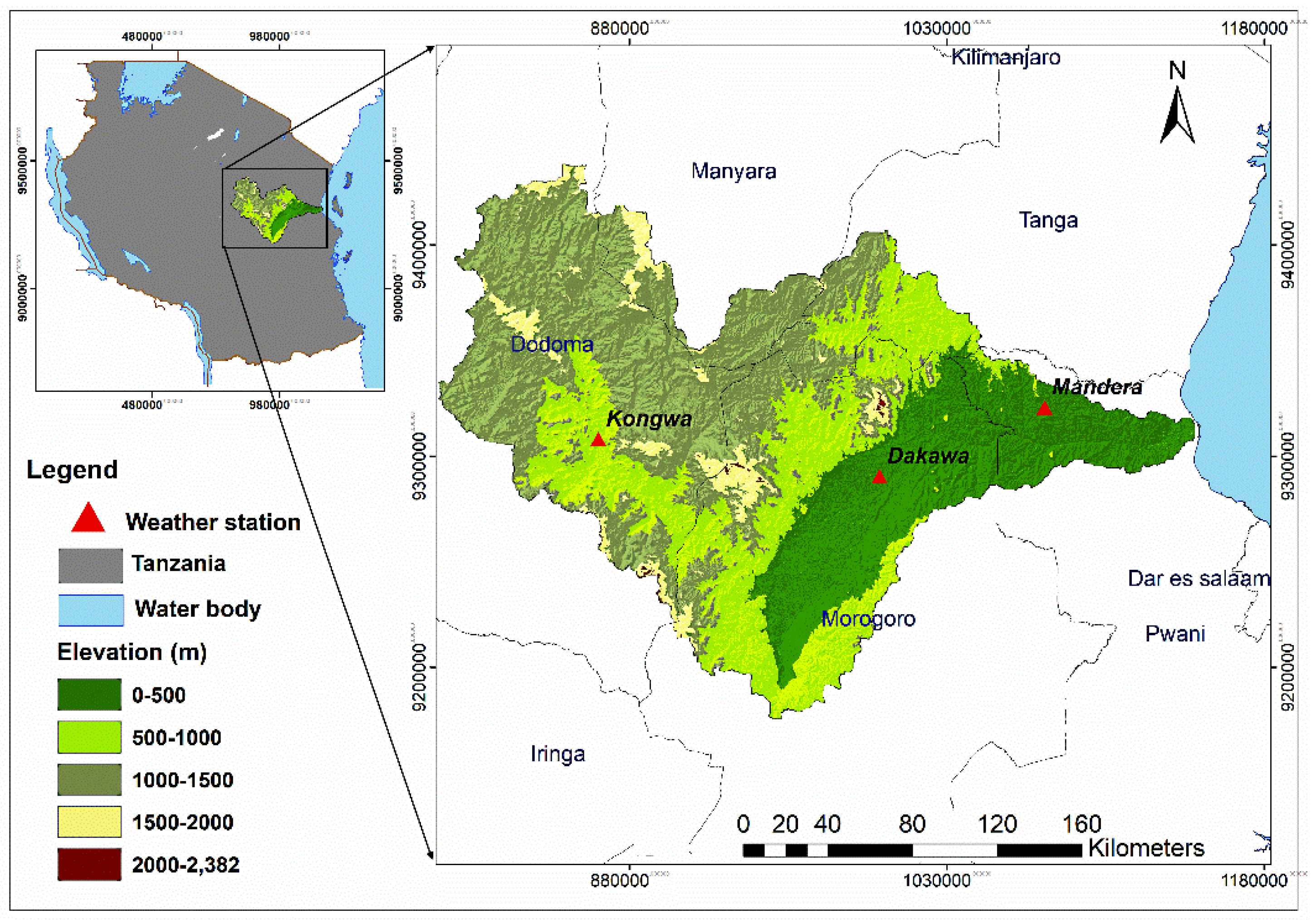
2.1. Study Area

The study location of the Wami River Basin (Figure 1) ranges between 5–7° S and 36–39° E covering the semi-arid parts in central Tanzania. It covers 41,167 km² and is characterized by humid inland swamps linked to the Indian Ocean. The basin topographically ranges from 2–2370 m above sea level. Kinyasungwe, Mkondoa, and Wami are three major sub-catchments forming the Wami River Basin [48]. Climatic conditions in the Wami River Basin are both spatially and seasonally variable with an average annual rainfall estimated to be 550–750 mm in the highlands near Dodoma, 900–1000 mm in the middle parts of the basin near Dakawa and at the river’s estuary in Bagamoyo [49]. The lowlands are warm, whereas the highlands are cold. The Wami River Basin is comprised of five basin draining zones—(i) upland plains, (ii) mountain torrents, (iii) inland plains, (iv) rejuvenated cascades, and (v) coastal plains—which characterize the topography of the study area. The river’s path varies: a relatively straight and confined pattern is observed in elevated and mountainous areas, but a meandering system dominates the coastal and inland plains, interfered with in a few areas by minor cascades at certain gradient levels [50]. On the other hand, a cascade zone can be seen near Wami at Mandera, upstream from the bridge crossing on the Chalinze–Segera highway [51].

2.2. Land Use Change Analysis and Prediction

Land use assessment was carried out based on images from Landsat-5, Landsat-7, and Landsat-8. The USGS Global Visualization Viewer (https://glovis.usgs.gov) provided the images, from which those with 30 m resolution and less cloud cover were chosen using Path/Row 168/64, 168/65, 166/64, 167/64, and 167/65 (

Table 1. Details of Landsat images used in the study.

Year	Satellite	Sensor	Path/Row	Resolution (m)	Acquisition Date	Cloud Cover
2000	Landsat 5	TM	168/64	30	10 October 2000	1%
	Landsat 5	TM	168/65	30	10 October 2000	4%
	Landsat 5	TM	166/64	30	21 January 1997	12%
	Landsat 7	ETM	167/64	30	07 July 2000	5%
	Landsat 7	ETM	167/65	30	07 July 2000	2%
2016	Landsat 8	OLI	168/64	30	22 October 2016	0.06%
	Landsat 8	OLI	168/65	30	22 October 2016	0.07%
	Landsat 8	OLI	167/64	30	16 September 2017	1.92%
	Landsat 8	OLI	167/65	30	16 September 2016	2.42%
	Landsat 8	OLI	166/64	30	26 January 2016	17.44% (not in the study area)

). The image classification was hybrid, comprised of both unsupervised and supervised classification techniques [52,53]. The Iterative Self-Organizing Data Analysis (ISODATA) clustering algorithm carried out unsupervised classification, while the Maximum Likelihood Classification (MLC) algorithm was engaged for supervised classification [54,55]. The delineated types were woodland, bushland, wetland, cultivated land, grassland, built-up area, water, and natural forest (

Table 2. Land use classes classification scheme.

Class	Descriptions
Bushland	Mainly comprised of plants that are multi-stemmed from a single root base.
Woodland	An assemblage of trees with canopy ranging from 20–80% but which may, on rare occasions, be closed entirely.
Wetland	Low-lying, uncultivated ground where water collects; a bog or marsh.
Cultivated land	Crop fields and fallow lands.
Built-up area	Residential, commercial, industrial, transportation, roads, and mixed urban.
Grassland	Mainly composed of grass.
Natural forest	A continuous stand of trees, many of which may attain a height of 50 m; includes natural forest, mangroves, and plantation forests.
Water	River, open water, lakes, ponds, and reservoirs.

). To improve classification accuracy, post-classification refinement was used [56]. The mixed pixels problem was later addressed by visual interpretation. Later, the stratified random method was used to assess the accuracy for both of two land use maps in the study area representing different land use classes. Moreover, the non-parametric Kappa test was used for classification accuracy, in order to account for the diagonal and confusion matrix elements [57].

Simulation of future land use change was based on CA–Markov chain analysis. The CA–Markov chain is a statistical tool which can define the chance of the land use changing from one date to another by establishing a transitional probability matrix between the first period and second period, based on the neighborhood effects [58,59,60]. The CA–Markov model was developed using the IDRISI Selva 17.0 software following two significant steps: first, to calculate the conversion probability, a conversion area matrix followed by layers of conditional probability is constructed by employing Markov chain analysis; the second stage is spatial description of the land use analysis, simulated by a CA spatial operator and multi-criteria evaluation (MCE) to predict and simulate the future land use change [61,62]. The classified land use maps for 2000 (which represents the past) and 2016 (which represents the present) were used as input data into the model, in order to predict the expected change for the year 2032. We performed model validation by comparison of the 2016 simulated land use map with the actual satellite land use map based on Kappa statistics [63]. The VALIDATE tool was used to compute the Kappa statistics for the projected land use and Kappa index >70% indicates a valid model [64].

2.3. Soil and Water Assessment Tool (SWAT) Model

The SWAT model was applied in the Wami River Basin to assess the effects of land use changes on hydrological components. A significant number of SWAT models have been applied to study hydrology in watersheds in different areas of the world. More details about the SWAT model can be found in Arnold et al. [65] and at http://swat-model.tamu.edu/. The SWAT model input data included a Digital Elevation Model (DEM), climate data, soil data, and a land use map. The DEM was obtained from the Shuttle Radar Topography Mission (SRTM) data set with a resolution of 30 m × 30 m. The soil data was obtained from the FAO with 1 km resolution. Land use data for two periods (2000 and 2016) and the projected land use (2032) maps were used to assess the effects of land use changes on the hydrology of the Wami River Basin. The observed climatic data, including daily rainfall and minimum and maximum temperatures values from 1990–2012 for the Wami River Basin, were obtained from the Tanzania Meteorological Agency (TMA). Daily runoff data from the Mandera gauge station (at the outlet of the catchment) from 1990–2012 was collected from the Ministry of Water, Tanzania. The SWAT 2012 version was used, based on the slope, soil data, and land use. The study area was divided into 23 sub-basins, which were later subdivided into 71 HRUs. The SWAT model simulates the land stage of the hydrological cycle established on the water balance equation [65]. The Soil Conservation Service Curve Number (SCS CN) method was employed in the study to compute the runoff, using Equation 2 [66,67,68]:

$$S{W}_t=S{W}_O+{\displaystyle \sum }_{i=1}^t\left(R_{day}-Q_{surf}-E_a-W_{sweep}-W_{gw}\right)$$

(1)

where $S{W}_t$ is the final water content (mm), $S{W}_0$ is the initial water content (mm), t is the time (days), $R_{day}$ is the amount of precipitation on a specific day (mm), $Q_{surf}$ is the runoff amount on a specific day (mm), $E_a$ is the evapotranspiration amount on specific day (mm),$W_{sweep}$ is the amount of water percolation into the vadose zones on a specific day (mm), and $W_{gw}$ is the return amount of flow on a specific day (mm).

$$Q_{surf}=\frac{{\left(R_{day}-I_a\right)}^2}{\left(R_{day}-I_a+S\right)}$$

(2)

where $Q_{surf}$ is the daily surface runoff (mm), $R_{day}$ is the precipitation depth for the day (mm), and $S$ is the retention parameter (mm). The retention parameter ($S$) is given by the equation

$$S=25.4\left(\frac{1000}{CN}-10\right)$$

(3)

where $S$ is the drainable volume of soil water per unit area of the saturated thickness (mm/day) and $CN$ is a curve number. $I_a$ is usually given as 0.2S. Therefore, Equation 2 becomes

$$Q_{surf}=\frac{{\left(R_{day}-0.2S\right)}^2}{\left(R_{day}+0.8S\right)}$$

(4)

Nineteen flow parameters were selected to detect the SWAT sensitive parameters, based on the literature [69,70,71,72,73,74]. Global sensitivity analysis [73,75,76,77] was employed in SWAT-CUP 2012 version 5.1.4 by allowing each parameter to be individually varied at a time [78]. To analyze the significance sensitivity, the p-value and t-Stat were used [73,75,76,77]: a high t-test value means high sensitivity, whereas a lower p-value indicates higher significance [73,75,77]. Model calibration is a process of adjusting model parameters, within the suggested ranges, based on observed data to approve the same response over time [78,79,80], and validation is the process of proving the representation of the parameters by simulating the observed data with an independent data set exclusive of changing model parameters [78,79,80]. The Sequential Uncertainty Fitting (SUFI-2) algorithm was used to carry out calibration and validation, as established in the SWAT-CUP user manual [75]. SUFI-2 is a semi-automated calibration and uncertainty analysis algorithm [81] that accounts for all sources of uncertainty, including uncertainty in the driving variables (e.g., rainfall), conceptual model, parameters and measured data [69,79,80]. SUFI-2 is the most popular calibration and uncertainty analysis program and, has been used in many studies [69,77,80,82]. The data set was split into a warm-up period (1990–1999), a calibration period (2000–2006), and a validation period (2007–2012). There are several indices available to check the performance of the SWAT model; the following were used to evaluate the performance of the SWAT model, as recommended by Moriasi et al. [83]:

$$\mathrm{Coefficient} \mathrm{of} \mathrm{Determination} R^2={\left[\frac{{{\displaystyle \sum }}_{i=1}^n\left(Ob{s}_i-Ob{s}_{avr}\right)\ast \left(Si{m}_i-Si{m}_{avr}\right)}{\sqrt{\left[{{\displaystyle \sum }}_{i-1}^n{\left(Ob{s}_i-Ob{s}_{avr}\right)}^2\right]}\ast \left[\sqrt{{{\displaystyle \sum }}_{i-1}^n{\left(Si{m}_i-Si{m}_{avr}\right)}^2}\right]}\right]}^2$$

(5)

$$\mathrm{Nash}–\mathrm{Sutcliffe} \mathrm{Efficiency} NSE=1-\left[\frac{{{\displaystyle \sum }}_{i=1}^n{\left(Ob{s}_i-Si{m}_i\right)}^2}{{{\displaystyle \sum }}_{i-1}^n{\left(Ob{s}_i-Si{m}_{avr}\right)}^2}\right]$$

(6)

$$\mathrm{Percentage} \mathrm{Bias} PBIAS=\left[\frac{{{\displaystyle \sum }}_{i=1}^n\left(Ob{s}_i-Si{m}_i\right)\ast 100}{{{\displaystyle \sum }}_{i=1}^{n}Ob{s}_i}\right]$$

(7)

$$\mathrm{Observation} \mathrm{standard} \mathrm{deviation} \mathrm{ratio} RSR=\frac{RMSE}{STDE{V}_{obs}}=\frac{\left[\sqrt{{{\displaystyle \sum }}_{i=1}^n{\left(Ob{s}_i-Si{m}_i\right)}^2}\right]}{\left[\sqrt{{\displaystyle \sum }{\left(Ob{s}_{i=1}-Ob{s}_{avr}\right)}^2}\right]}$$

(8)

The detailed land use maps (2000 and 2016) and the predicted land use map (2032) were used individually, whereas the other SWAT model inputs were the same as those used to analyze the basin’s response to land use change. The simulated results were used to assess the effects of historical and future land use changes on water hydrology and to measure the input of changes in separate land use types to changes in hydrological components at the catchment.

2.4. Pearson Correlation and Partial Least Squares Regression

The relationship between land use change and hydrological components was assessed using the pairwise Pearson correlation [39,41,74]. Pearson correlation analysis was adopted to analyze the linear correlations between land use change (dependent variables) and hydrological components (independent variables). Significant values were determined by a 95% confidence interval from the sample size, n equal to four (independent variables), and the Pearson correlation coefficient. Thus, land use change influences the hydrological components more firmly as the Pearson correlation coefficient value approaches 1. Moreover, the hydrological effects of separate land use changes were investigated using correlation analysis by the Partial Least Squares Regression (PLSR) model. PLSR is a multivariate analysis method (Equation 9) which combines and generalizes features from primary element analysis and multiple regressions [84]. PLSR forecasts a dependent variable(s) set from an independent variables set [84,85,86,87,88]. One of the benefit features of PLSR is that the relations between the dependent and independent variables can be concluded from the weights and regression coefficients of single dependent variable in the furthermost independent components [85,86]. Thus, it is possible to control which dependent variable strongly relates with independent variables [88].

Using multiple regression, changes in hydrological components between two land use maps in 2000 and projected 2032, respectively, were related to changes of land use to quantify the effect of individual land use at the basin scale. Dependent variables were the changes for eight land use classes (i.e., natural forest, woodland, bushland, grassland, water, wetland, cultivated land and built-up area) while independent variables (responses) were changes for four hydrological components (i.e., surface runoff, groundwater flow, evapotranspiration and water yield). The PLSR models were created to recognize the key land use types that control hydrological components. To reduce the drawback of over-fitting, the suitable number of components of individual PLSR model was determined by cross-validation to attain an optimum balance among the described variation in the response and the projecting ability of the model (goodness of prediction: Q²). In PLSR modelling, the significance of a predictor for both the dependent and the independent variables is set by the variable importance for the projection (VIP), with large VIP values are the best significant for describing the dependent variable.

The percentage of variance and cross-validated goodness of prediction (Q²) described for the dependent variables (hydrological components), together with the cross-validated root mean squared error as the change among the predicted and observed values of each individual pass, were analyzed for each model. The regression coefficients of the PLSR models were used to express the direction of the correlation between the changes in individual land use types and hydrological components. XLSTAT was used to perform the statistical analysis of the dataset [41].

$$y=b_0+b_1{x}_1+b_2{x}_2+b_3{x}_3+\cdots +b_i{x}_i.$$

(9)

where $y$ is the dependent variable, $b_0$ is the intercept, x is the independent variables from 1 to i, and b is the coefficients of the x variables.

3. Results and Discussion

3.1. Accuracy Assessment and CA-Markov Validation

The accuracy results, including accuracy per specific land use class (i.e., producer accuracy (PA) and user accuracy (UA)), are presented in

Table 3. Land use accuracy at Wami River Basin.

	2000		2016
Land Use	PA	UA	UA	PA
Natural Forest	98.68	94.46	98.59	99.18
Woodland	86.05	95.07	98.68	99.53
Bushland	89.16	84.95	99.19	98.53
Grassland	98.47	89.66	99.40	97.62
Water	100	99.68	100	100
Wetland	95.26	90.29	99.33	95.68
Cultivated land	87.13	92.10	99.10	99.72
Built-up area	98.35	99.01	97.03	98.56
Overall Accuracy (%)	91.87		99.01
Kappa coefficient	0.90		0.99

. The overall accuracy was 91.87% and 99.01% for the 2000 and 2016 maps, respectively. The Kappa coefficient was above 0.90 for the two classified images. According to Anderson et al. [89], the level of accuracy in the classification of land use classes from remote sensing data must be at a minimum of 85%, while the Kappa coefficient must be higher than 80% [90]. Hence, the data set showed an excellent agreement with the image and the ground truths. CA–Markov validation was achieved, with a Receiver Operating Characteristic (ROC) value of 87.5%. The Kappa statistics values such as Kno (86.20%), Klocation (83.3%), KlocationStrata (89.8%) and Kstandard (81.9%) were also above 80%, which shows the excellent capacity of the model to simulate the 2032 land use [91,92].

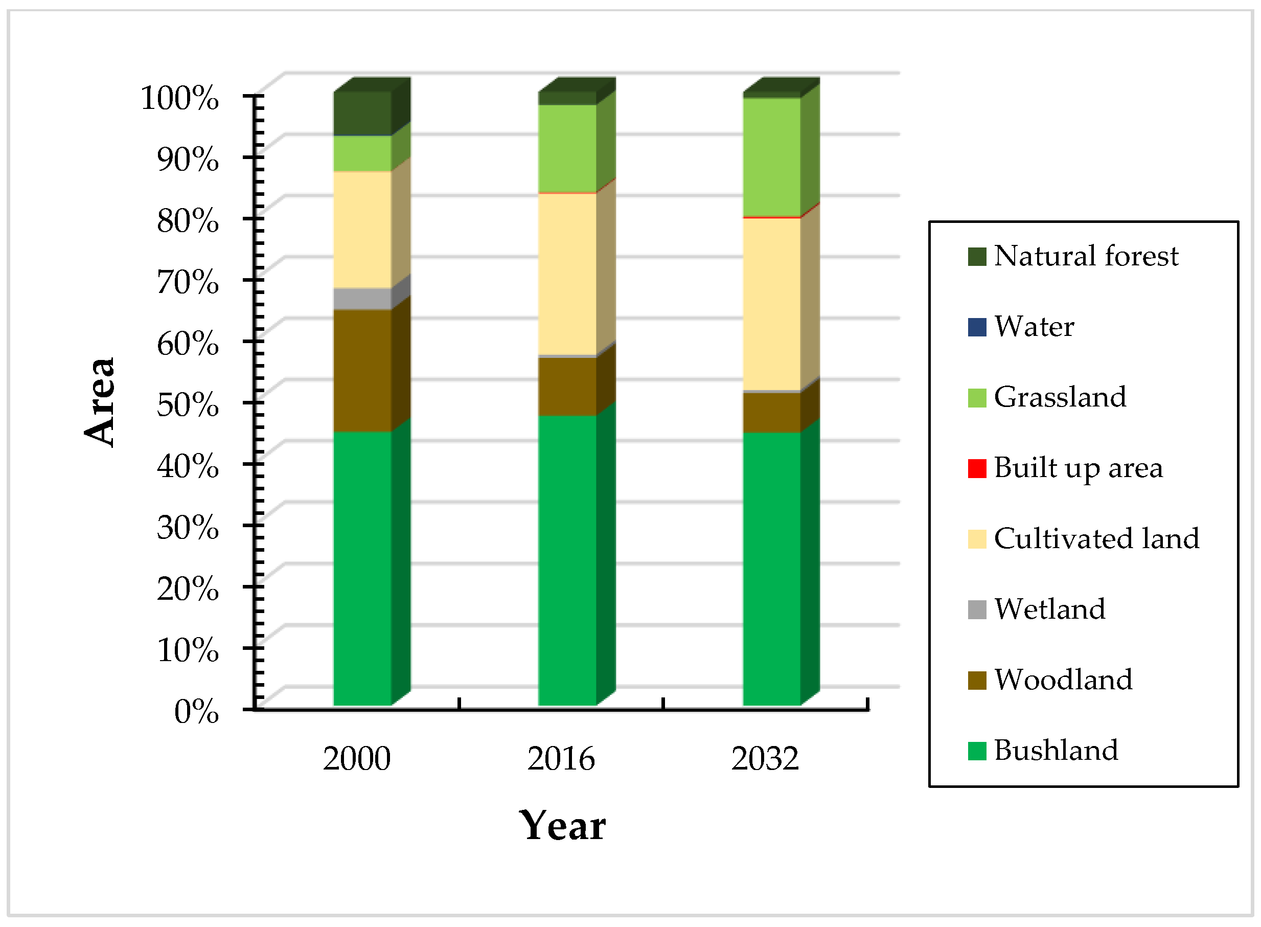
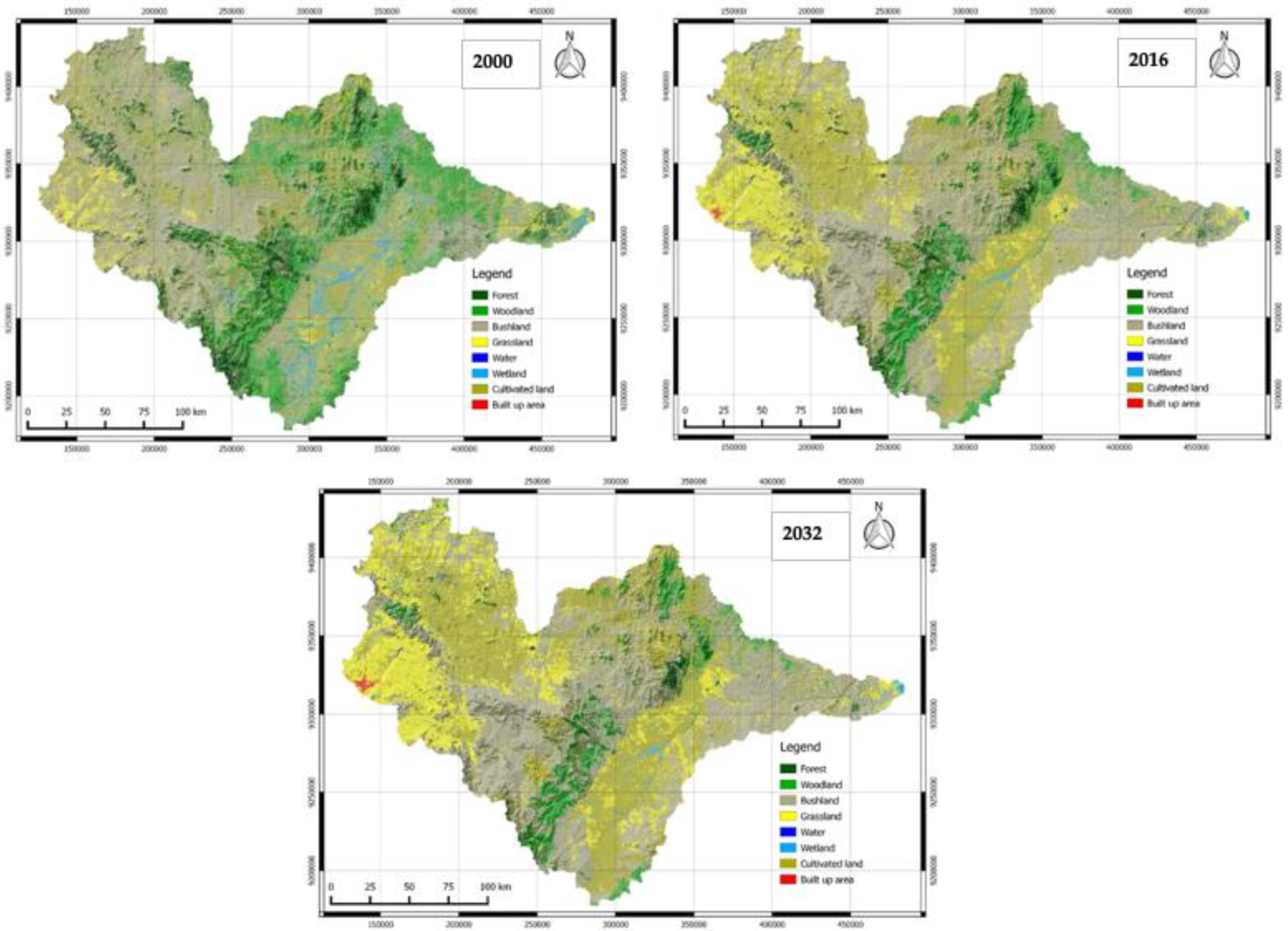
3.2. Land Use Change Analysis

The land use situations of the Wami River Basin between 2000 and 2032 are shown in

Table 4. Areas of individual land use classes in the years 2000, 2016, and 2032 (projected).

Year	2000		2016		2032		Rate of Change
Land Use	Area (km2)	%	Area (km2)	%	Area (km2)	%	(km2/year)
Natural forest	2892.40	6.99	863.63	2.09	424.05	1.02	−126.80
Woodland	8252.20	19.93	3903.58	9.43	2676.77	6.46	−310.62
Bushland	18,416.20	44.48	19,529.85	47.17	18,393.29	44.42	79.55
Grassland	2376.24	5.74	5901.68	14.25	7990.64	19.30	251.82
Water	76.88	0.19	8.46	0.02	7.23	0.019	−4.89
Wetland	1491.62	3.50	223.35	0.54	193.19	0.47	−90.59
Cultivated land	7891.65	19.05	10,907.99	26.34	11,603.20	28.02	215.45
Built-up area	8.81	0.02	67.46	0.16	117.63	0.28	4.19
Total	41406	100	41406	100	41406	100

,

Table 5. Results of the land use classification for 2000, 2016, and 2032 (projected) images, showing area change and percentage.

Land Use	2000–2016		2016–2032
	Area Change(km2)	%	Area Change (km2)	%
Natural forest	−2028.77	−4.90%	−439.58	−1.07%
Woodland	−4348.62	−10.50%	−1226.81	−2.97%
Bushland	1113.65	+2.69%	−1136.56	−2.75%
Grassland	3525.44	+8.51%	2088.96	+5.05%
Water	−68.42	0.17%	1.23	−0.001%
Wetland	−1268.27	−2.96%	−30.16	−0.07%
Cultivated land	3016.34	+7.29%	695.21	+1.68%
Built-up area	58.65	+0.14%	50.17	+0.12%

and Figure 2, while the spatial distribution of all land use is represented in Figure 3. During 2000–2016, a small amount of land use change happened in the basin; further, these changes are anticipated to continue in 2032. For example, grassland increased from 5.74% in 2000 to 14.25% in 2016 and is predicted to continue to increase to 19.30% by 2032 (Table 4). Cultivated land area expanded from 19.05% in 2000 to 26.34% in 2016 and continued increasing to 28.02% in 2032. Similarly, built-up areas increased between 2000 and 2016 (0.02% to 0.16%), and are expected to increase to 0.28% by 2032. Moreover, bushland increased from 44.48% in 2000 to 47.17% in 2016, but is expected to decrease to 44.42% in 2032. Nevertheless, the yearly expansion percentage of grassland until 2032 is higher than cultivated land, followed by bushland and built-up areas. Net loss was observed in natural forests, woodland, wetlands, and water. Natural forest decreased from 6.99% in 2000 to 2.09% in 2016 and continued to decrease to 1.02% in 2032 (Table 4). Woodland decreased from 19.93% in 2000 to 9.43% in 2016 and continued to decrease to 6.46% in 2032. Similarly, the extent of wetland decreased between 2000 and 2016 (3.50% to 0.54%), and is expected to decrease in to 0.47% in 2032. Moreover, water decreased from 0.19% in 2000 to 0.02% in 2016; it is expected to remain constant in the period up to 2032. The annual reduction rate of woodland until 2032 was greater than that of natural forests, followed by wetlands and water. These results are in agreement with a previous study in the basin [53].

3.3. Sensitive Parameters.

The sensitivity analysis results identified six sensitive parameters controlling the output variable (

Table 6. Sensitive flow parameters and their rank.

Rank	Parameter	Parameter Definition	Min	Max	Fitted Value
1	R_CN2.mgt	SCS runoff curve number	−0.3	0.3	−0.023000
2	SOL_AWC.sol	Available water capacity of the soil layer	−0.8	0.8	0.210667
3	V_GW_DELAY.gw	Groundwater delay	0	600	109.000000
4	V_ALPHA_BF.gw	Baseflow alpha factor	0	1.011	0.652095
5	GWQWN.gw	Threshold depth of water in the shallow aquifer required for return flow to occur	0	2000	1730.000000
6	ESCO.hru	Soil evaporation compensation factor	0	1	0.711667

). The parameters were adjusted to suit the ranges, until a satisfactory agreement was obtained between observed and simulated flows. Parameter values (upper and lower bound, and fitted value) used for model sensitivity analysis were found within the rage of the suggested SWAT user’s manual [93]. The three most sensitive parameters were R_CN2.mgt, SOL_AWC.sol, and V_GW_DELAY.gw.

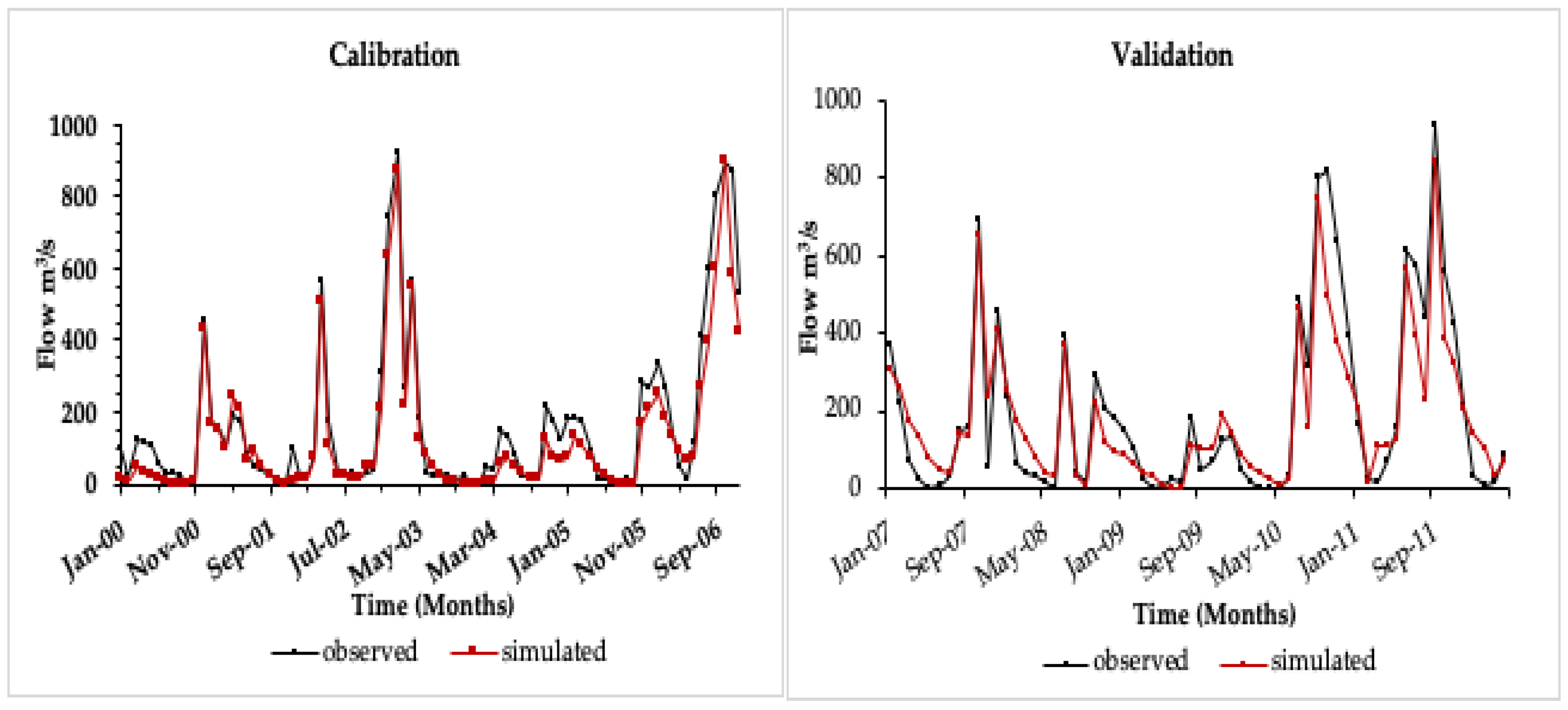
3.4. Calibration and Validation

According to Niraula et al. [42], a hydrological model should be calibrated spatially; hence, the SWAT model was calibrated using three gauging stations (Figure 1). Calibration (2000–2007) and validation (2007–2012) were performed using monthly data, and the result is presented in

Table 7. Model performance statistics for the calibration and validation periods.

Period		Average Monthly Flow(m3/s)		Evaluated Statistics
		Observed	Simulated	NSE	RSR	PBIAS	R2
Jan 2000–Dec 2006	Calibration	158.14	150.30	0.71	0.59	5.0	0.93
Jan 2007–April 2012	Validation	176.84	168.10	0.65	0.54	4.9	0.83

. Figure 4 shows comparative results of observed and simulated flows for the duration of calibration and validation. The parameter values for NSE, RSR, PBIAS, and R² were, respectively, estimated as 0.65, 0.59, 5.0, and 0.69 in calibration, and 0.71, 0.54, 0.49, and 0.73 in validation. The simulation reflected the observed flow rationally, indicating a good performance of model in simulating the hydrological impacts of land use changes over the 2000 to 2032 periods [72,74,76,83].

The achieved R² (0.93 for calibration and 0.83 for validation) values express good evenness between the observed and simulated data [72,74,76,83]. NSE above 0.60, PBIAS < 10% and RSR < 0.6 were also achieved while positive values of PBIAS indicate the under estimation of the model.

3.5. Impacts of Land Use Changes in Hydrological Components

Investigation of the variations in the hydrological components influenced by land use changes showed effects on the components (

Table 8. Hydrological component change due to land use.

Hydrological Component	2000	2016	2032	2000–2016	2016–2032
Surface runoff (mm)	64.61	68.84	71.26	+4.23	+2.42
Groundwater flow (mm)	87.45	86.76	85.24	–0.69	–1.52
Evapotranspiration (mm)	511.8	508.7	507.6	–3.1	–1.1
Water yield (mm)	168.38	171.63	172.77	+3.25	+1.14

). The analysis focused on hydrological components including surface runoff, groundwater flow, evapotranspiration and water yield. The results are presented in Table 7, from which it can be seen that the hydrological components were affected differently, while surface runoff was the most significant contributor to streamflow in the Wami River Basin. With land use 2000, the results for the hydrological components were as follows: surface runoff, 64.61 mm; groundwater flow, 87.45 mm; evapotranspiration, 511.8 mm; and water yield, 168.38 mm. Moreover, the results showed that, with land use 2016, the surface runoff, groundwater flow, evapotranspiration, and water yield were 68.84 mm, 86.76 mm, 508.7 mm, and 171.63 mm, respectively, while those for 2032 (projected) were 71.26 mm, 85.24 mm, 507.6 mm, and 171.77 mm, respectively. Furthermore, between 2000 and 2016, the surface runoff increased by 4.23 mm while the water yield increased by 3.25 mm, while groundwater decreased by 0.69 mm and evapotranspiration decreased by 3.1 mm over the same period. During the study period (2016–2032), an increasing trend was observed in surface runoff (by 2.42 mm) and water yield (by 1.14 mm), while a decreasing trend was observed in groundwater flow (by 1.52 mm) and evapotranspiration (by 1.1 mm).

3.6. Impacts of Individual Land Use Changes in Hydrological Components

The pairwise relationships of the eight land use types and hydrological components are presented in

Table 9. Pairwise Pearson correlation for changes in land use types and hydrological components between 2000 and 2032 periods.

Variable	NF	WL	BL	GL	WT	WTL	CL	BLT	SUR_Q	GW_Q	ET	WYLD
NF	1.000
WL	0.999	1.000
BL	−0.329	−0.289	1.000
GL	−0.978	−0.986	0.127	1.000
WT	0.986	0.978	−0.483	−0.930	1.000
WTL	0.989	0.982	−0.466	−0.937	1.000	1.000
CL	−1.000	−0.999	0.322	0.980	−0.984	−0.988	1.000
BLT	−0.952	−0.964	0.025	0.995	−0.887	−0.897	0.955	1.000
SUR_Q	−0.980	−0.988	0.136	1.000	−0.933	−0.940	0.982	0.994	1.000
GW_Q	0.843	0.865	0.231	−0.936	0.740	0.754	−0.847	−0.967	−0.933	1.000
ET	0.996	0.999	−0.247	−0.993	0.968	0.973	−0.997	−0.975	−0.994	0.886	1.000
WYLD	−0.996	−0.999	0.249	0.992	−0.968	−0.973	0.997	0.975	0.993	−0.885	−0.986	1.000

NF—Natural forest, WL—Woodland, BL—Bushland, GL—Grassland, WT—Water, WTL—Wetland, CL—Cultivated land, BLT—Built-up area, SUR_Q—Surface runoff, GW_Q—Groundwater flow, ET—Evapotranspiration, WYLD—Water yield.

. Based on the results, nearly all land use types showed a strong relationship with the individual hydrological components. For example, natural forest and woodland both showed negative (but significant) correlations with water yield and surface runoff, and positive correlations with groundwater flow and ET. Bushland had a positive correlation with water yield, surface runoff, and groundwater, but a negative correlation with ET. Furthermore, it was observed that grassland, cultivated land, and built-up areas had significant positive correlations with water yield and surface runoff, while their correlations with groundwater and ET were negative. However, water and wetland had significant negative correlations with surface runoff and water yield, and significant positive correlations with groundwater and ET.

The results of the PLSR model for hydrological components in the Wami River Basin are given in

Table 10. Results of the Partial Least Squares Regression (PLSR) model of the hydrological components in the Wami River Basin.

Response Variable Y	Variation in Response	Q2	Component	Explained Variability in Y (%)	Cumulative Explained Variability in Y (%)	Root Mean PRESS	Q2 cum
Hydrological components(SURQ, GWQ, ET, WYLD)	0.975	0.916	1	95.1	95.1	0.216	0.955
			2	3.1	98.2	0.342	0.988
			3	1.6	99.8	0.446	0.992
			4	0.2	100	0.672	0.995

Note: The bold number indicates the number of factors required to fit the PLSR model; the minimum Root Mean PRESS shows the number of predictors needed to explain the model (SAS Institute Inc, 2017).

and a summary of the PLSR weights and variable importance of the projected values (VIP) of the hydrological components is given in

Table 11. Variable importance for the projection (VIP) values and PLSR weights of hydrological components in the Wami River Basin.

	Hydrological Components (SURQ, GWQ, ET & WYLD)
	VIP	W*1	W*2	W*3
Natural forest	1.074	−0.380	0.307	0.909
Woodland	1.083	−0.383	0.349	0.360
Bushland	0.126	−0.045	0.909	0.389
Grassland	1.100	0.219	−0.015	−0.462
Water	1.018	−0.360	0.455	0.427
Wetland	1.026	−0.363	0.436	0.431
Cultivated land	1.076	0.380	−0.407	−0.452
Built-up area	1.096	0.387	−0.302	−0.460

Note: The bold numbers are values greater than 0.3; the positive and negative signs indicate the sign of the loadings in the PLSR model.

. The PLSR model Q², cumulative, and variation in the response values were above 0.60, signifying that the model was correctly predicted. The minimum Root Mean Press (predicted residual sum of squares) was used to obtain three components of water balance in the Wami River Basin. The variance of changes in water balance for the 1^st, 2^nd, and 3^rd components was explained in the cumulative model by 95.1%, 98.2%, and 99.8%, respectively (Table 10). The explained variance did not significantly increase with additional components (Table 11).

The first component was dominated by natural forest, woodland, water and wetland on the negative side, and by built-up area and cultivated land on the positive side. Moreover, the second component was dominated by natural forest, woodland, bushland, water and wetland on the positive side, and cultivated land and built-up area on the negative side. The last component was dominated by all land classes, where the negative side included grassland, built-up area and cultivated land, while the positive side included natural forest, woodland, bushland, water and wetland. The results of the relative importance of predictors of the model showed that bushland (VIP < 1) had less significance and that bushland and grassland were relatively less important in affecting water balance components, compared to other land use types.

Furthermore, the PLSR coefficients showed the effects of individual land use types on hydrological components in the periods from 2000 to 2032 in the Wami River Basin, which are given in

Table 12. PLSR coefficients presenting the effects of different land use types on hydrological components between 2000 and 2032 (projected) in the Wami River Basin.

Model	Variable	NR	WL	BL	GL	WT	WL	CL	BT
PLSR 1	SURQ	−0.980	−0.988	−0.136	−1.000	−0.933	−0.940	0.982	0.994
	GWQ	0.843	0.865	0.231	0.936	0.740	0.754	−0.847	−0.967
	ET	0.996	0.999	0.247	0.993	0.968	0.973	−0.997	−0.975
	WYLD	−0.996	−0.999	−0.249	−0.992	−0.968	−0.973	0.997	0.975

NF—Natural forest, WL—Woodland, BL—Bushland, GL—Grassland, WT—Water, WTL—Wetland, CL—Cultivated land, BLT—Built-up area. Note: The positive and negative signs reveal the influence position.

. The regression coefficients indicated that natural forest, woodland, bushland, grassland, water and wetland influenced water yield and surface runoff negatively, while the effects of built-up area and cultivated land on these components were positive. Moreover, the regression coefficient results revealed that cultivated land and built-up area influenced groundwater flow and evapotranspiration negatively, while the effects of natural forest, woodland, bushland, grassland, water and wetland on these components were positive.

4. Discussion

The main objectives of this study were to investigate the effects of land use change on various elements of the hydrological processes in the Wami River Basin. The change of different land use types occurred in different directions and degrees during the study period. For example, natural resource decreased except for grassland while increasing changes were observed in cultivated land and built-up area. By analyzing land use changes, this paper indicated that the Wami River Basin was experiencing cultivated land and built-up area development during the study period. The land use pattern observed agrees with findings from Dickens [94] and Anderson [95] in which it was found that challenges for river conservation and management include expansion of irrigated agriculture and increasing domestic water supply withdrawal due to population increase. Furthermore, the basin was affected by the Southern Agricultural Growth Corridor of Tanzania Project with the aim of accelerated agricultural expansion and agricultural intensification [96]. Thus, irrigation is desirable and comes at the cost of already stressed fresh water supplies [97].

Simulating a land use change in Wami River Basin revealed the changes in basin hydrological processes. From the study, it is evident that land use has changed across the basin since 2000 and is expected to continue in 2032, while the effects of land use changes on the hydrological components were observed. The increase of bushland, grassland, built-up areas and cultivated land, accompanied by a decrease of the natural forests, woodland, water and wetlands during the study period increased water yield and surface runoff while reducing the groundwater flow and evapotranspiration. The ET is the key element in understanding the effect of change in land use on water production, and in this study a significant decrease was shown, which could be caused by increase in grassland [98]. The results agree with Neitsch et al.’s [93] statements, showing that the SWAT model computes the ET based on the maximum plant transpiration rate, canopy water evaporation intercepted and the maximum soil evaporation rate.

The PLSR results demonstrated that all land uses are significant and were relatively important in affecting water balance components, except for bushland and grassland. Therefore, in terms of water stability, the natural forest, woodland, wetland, cultivated land and built-up area should be regulated to a rational level to decrease the related impact on hydrological components. Despite relatively small changes in runoff generation due to the land use change, the findings suggest that increasing cultivated land and the built-up area in the Wami River Basin can cause severe threats in the future [55]. This will be more complicated with the current rapid population growth, climate change and economic growth within the basin [99]. The results can be used to identify and prioritize the implementation of best management practices in the most vulnerable areas to protect the natural resource in the basin [100]. Additionally, this study showed the potential of using a hydrologic modelling framework for a data-scarce basin in Tanzania. The use of Landsat images produced precise land use types in this analysis and showed the land use change in the basin. These results can be used to identify and highlight the application of best management practices in the most exposed areas.

5. Conclusions

Effects of changes in land use classes due to hydrology components in the Wami River Basin were assessed using hydrological modeling and PLSR. It was found that the major land use changes that affected hydrology components in the basin were expansion of cultivation land, built-up area and grassland, and decline in natural forests and woodland during the study period. The VIP values for these land-use types are greater than 1, and hence they are considered of great importance for the prediction of changes in the hydrology components. It can be concluded from the analysis that cultivation land, built-up area and grassland is directly proportional to the surface run-off and water yield, but inversely proportional to the groundwater flow and evapotranspiration. Furthermore, the decline in other land use classes is directly proportional to the groundwater flow and evapotranspiration, but inversely proportional to the surface run-off and water yield. These findings provide baseline information for decision-makers and stakeholders concerning land and water resources for better planning and management decisions in the basin. The approach used in this study has attributed contributions of changes in land use to hydrological components and might be useful to predict hydrological consequences of land use changes to another basins. Therefore, more studies should be undertaken to examine the effects of land use changes with different temporal and spatial scale in future research.

References

1. Abdulkareem, J.H.; Sulaiman, W.N.A.; Pradhan, B.; Jamil, N.R. Relationship between design floods and land use land cover (LULC) changes in a tropical complex catchment. Arab. J. Geosci. 2018, 11, 376. [Google Scholar] [CrossRef]
2. Maharjan, A.; Bauer, S.; Knerr, B. Migration for Labour and Its Impact on Farm Production in Nepal; Centre for the Study of Labour and Mobility: Kathmandu, Nepal, 2013. [Google Scholar]
3. Wear, D.N.; Turner, M.G.; Naiman, R.J. Land cover along an urban-rural gradient: Implications for water quality. Ecol. Appl. 1998, 8, 619–630. [Google Scholar]
4. Hogan, M.C. Water Pollution. In Encyclopedia of Earth; Topic ed.; Cleveland, C.C., McGinley, M., Eds.; National Council on Science and the Environment: Washington, DC, USA, 2010. [Google Scholar]
5. Torbick, N.; Hession, S.; Hagen, S. Mapping inland lake water quality across the lower peninsula of Michigan using Landsat TM imagery. Int. J. Remote Sens. 2013, 34, 7607–7624. [Google Scholar] [CrossRef]
6. Noori, H.; Siadatmousavi, M.; Mojaradi, B. Assessment of sediment yield using RS and GIS at two sub-basins of Dez Watershed, Iran. Int. Soil Water Conserv. Res. 2016, 4, 199–206. [Google Scholar] [CrossRef] [Green Version]
7. Khare, D.; Patra, D.; Mondal, A.; Kundu, S. Impact of landuse/land cover change on run-off in the catchment of a hydro power project. Appl. Water Sci. 2017, 7, 23–35. [Google Scholar] [CrossRef]
8. Notter, B.; MacMillan, L.; Viviroli, D.; Weingartner, R.; Liniger, H. Impacts of environmental change on water resources in the Mt. Kenya Region. J. Hydrol. 2007, 343, 266–278. [Google Scholar]
9. Schneider, L.C.; Gil Pontius, R., Jr. Modeling land-use change in the Ipswich watershed, Massachusetts, USA. Agric. Ecosyst. Environ. 2001, 85, 83–94. [Google Scholar] [CrossRef]
10. Vörösmarty, C.J.; McIntyre, P.B.; Gessner, M.O.; Dudgeon, D.; Prusevich, A.; Green, P.; Glidden, S.; Bunn, S.E.; Sullivan, C.A.; Liermann, C.R.; et al. Global threats to human water security and river biodiversity. Nature 2010, 467, 555–561. [Google Scholar] [CrossRef]
11. Madulu, N. Environment, poverty and health linkages in the Wami river basin, A search for sustainable water resource management. Phys. Chem. Earth 2005, 30, 950–960. [Google Scholar] [CrossRef]
12. Wambura, J.J. Stream Flow Response to Skilled and Non-linear Bias Corrected GCM Precipitation Change in the Wami River Sub-basin, Tanzania. Br. J. Environ. Clim. Chang. 2014, 4, 389–408. [Google Scholar] [CrossRef]
13. Nobert, J.; Jeremiah, J. Hydrological Response of Watershed Systems to Land Use/Cover Change. A Case of Wami River Basin. Open Hydrol. J. 2012, 6, 78–87. [Google Scholar] [CrossRef]
14. Bates, B.C.; Kundezewicz, Z.W.; Wu, S.; Palutikof, J.P. Climate change and water: Technical paper of the Intergovernmental Panel for Climate Change (Geneva: IPCC Secretariat). Clim. Chang. 2008, 95, 96. [Google Scholar]
15. Todd, M.C.; Taylor, R.G.; Osborn, T.J.; Kingston, D.G.; Arnell, N.W.; Gosling, S.N. Uncertainty in climate change impacts on basin-scale freshwater resources–preface to the special issue: The QUEST-GSI methodology and synthesis of results. Hydrol. Earth Syst. Sci. 2011, 15, 1035–1046. [Google Scholar] [CrossRef] [Green Version]
16. Kepner, G.; Semmens, D.J.; Bassett, S.D.; Mouat, D.A.; Goodrich, D.C. Scenario analysis for the San Pedro River, analyzing hydrological consequences of a future environment. Environ. Monit. Assess. 2004, 94, 115–127. [Google Scholar] [CrossRef]
17. Christensen, N.A.; Wood, A.W.; Voisin, N.; Lettenmaier, D.P.; Palmer, R.N. The effects of climate change on the hydrology and water resources of the Colorado River basin. Clim. Chang. 2004, 62, 337–363. [Google Scholar] [CrossRef]
18. Tang, Z.; Engel, B.A.; Pijanowski, B.C.; Lim, K.J. Forecasting land use change and its environmental impact at a watershed scale. J. Environ. Manag. 2005, 76, 35–45. [Google Scholar] [CrossRef]
19. Hurkmans, R.T.W.L.; Terink, W.; Uijlenhoet, R.; Moors, E.J.; Troch, P.A.; Verburg, P.H. Effects of land use changes on streamflow generation in the Rhine basin. Water Resour. Res. 2009, 45, W06405. [Google Scholar] [CrossRef] [Green Version]
20. Li, Z.; Liu, W.Z.; Zhang, X.C.; Zheng, F.L. Impacts of land use change and climate variability in an agricultural catchment on the Loess Plateau of China. J. Hydrol. 2009, 377, 35–42. [Google Scholar] [CrossRef]
21. Park, J.Y.; Park, M.J.; Joh, H.K. Assessment of Miroc3.2 Hires Climate and Clue- S land Use change impacts on watershed hydrology using SWAT. Trans. ASABE 2011, 54, 1717–1724. [Google Scholar]
22. Perazzoli, M.; Pinheiro, A.; Kaufmann, V. Assessing the impact of climate change scenarios on water resources in southern Brazil. Hydrol. Sci. J. 2013, 58, 77–87. [Google Scholar] [CrossRef] [Green Version]
23. Shaw, S.B.; Marrs, J.; Bhattarai, N.; Quackenbush, L.J. Longitudinal study of the impacts of land cover change on hydrologic response in four mesoscale watersheds in New York State, USA. J. Hydrol. 2014, 519, 12–22. [Google Scholar] [CrossRef]
24. Hundecha, Y.; Bardossy, A. Modeling of the effect of land use changes on the runoff generation of a river basin through parameter regionalization of a watershed model. J. Hydrol. 2004, 292, 281–295. [Google Scholar] [CrossRef]
25. Wang, G.; Liu, J.; Kubota, J.; Chen, L. Effects of land-use changes on hydrological processes in the middle basin of the Heihe River, northwest China. Hydrol. Process. 2007, 21, 1370–1382. [Google Scholar] [CrossRef]
26. Zhang, X.; Cao, W.; Guo, Q.; Wu, S. Effects of landuse change on surface run-off and sediment yield at different watershed scales on the Loess Plateau. Int. J. Sediment Res. 2010, 25, 283–293. [Google Scholar] [CrossRef]
27. Rientjes, T.; Haile, A.; Kebede, E.; Mannaerts, C.; Habib, E.; Steenhuis, T. Changes in land cover, rainfall and stream flow in Upper Gilgel Abbay catchment, Blue Nile basin Ethiopia. Hydrol. Earth Syst. Sci. 2011, 15, 1979–1989. [Google Scholar] [CrossRef] [Green Version]
28. Warburton, M.; Schulze, R.; Jewitt, G. Hydrological impacts of land use change in three diverse South African catchments. J. Hydrol. 2012, 414–415, 118–135. [Google Scholar] [CrossRef]
29. Gumindoga, W.; Rientjes, T.H.M.; Haile, A.T.; Dube, T. Predicting streamflow for land cover changes in the Upper Gilgel Abay River Basin, Ethiopia: A TOPMODEL based approach. Phys. Chem. Earth Parts A/B/C. 2014, 76, 3–15. [Google Scholar] [CrossRef]
30. Kalantari, Z.; Lyon, S.; Folkeson, L.; French, H.; Stolte, J.; Jansson, P.; Sassner, M. Quantifying the hydrological impact of simulated changes in land use on peak discharge in a small catchment. Sci. Total Environ. 2014, 466–467, 741–754. [Google Scholar] [CrossRef]
31. Zhang, Y.; Schilling, K. Increasing streamflow and baseflow in Mississippi River since the 1940s: Effect of land use change. J. Hydrol. 2006, 324, 412–422. [Google Scholar] [CrossRef]
32. Bi, H.; Liu, B.; Wu, J.; Yun, L.; Chen, Z.; Cui, Z. Effects of precipitation and land use on run-off during the past 50 years in a typical watershed in Loess Plateau, China. Int. J. Sediment Res. 2009, 24, 352–364. [Google Scholar] [CrossRef]
33. Khoi, D.; Suetsugi, T. Impact of climate and land-use changes on hydrological processes and sediment yield: A case study of the Be River catchment, Vietnam. Hydrol. Sci. J. 2014, 59, 1095–1108. [Google Scholar] [CrossRef]
34. Akpoti, K.; Antwi, E.O.; Kabo-bah, A.T. Impacts of Rainfall Variability, Land Use and Land Cover Change on Stream Flow of the Black Volta Basin, West Africa. Hydrology 2016, 3, 26. [Google Scholar] [CrossRef] [Green Version]
35. Nietsch, S.L.; Arnold, J.G.; Kiniry, J.R.; Srinivasan, R.; Williams, J.R. Soil and Water Assessment Tool Input/Output File Documentation; Blackland Research Center: Temple, TX, USA, 2005. [Google Scholar]
36. Hernandez, M.; Miller, S.; Goodrich, D.; Goff, B.; Kepner, W.; Edmonds, C.; Jones, K. Modeling run-off response to land cover and rainfall spatial variability in semi-arid watersheds. Environ. Monit. Assess. 2000, 64, 285–298. [Google Scholar] [CrossRef]
37. Miller, S.; Kepner, W.; Mehaffey, M.; Hernandez, M.; Miller, R.; Goodrich, D.; Devonald, K.; Heggem, D.; Miller, W. Integrating landscape assessment and hydrologic modeling for land cover change analysis. J. Am. Water Resour. Assoc. 2002, 38, 915–929. [Google Scholar] [CrossRef]
38. Ghaffari, G.; Keesstra, S.; Ghodousi, J.; Ahmadi, H. SWAT-simulated hydrological impact of land-use change in the Zanjanrood basin, Northwest Iran. Hydrol. Process. 2010, 24, 892–903. [Google Scholar] [CrossRef]
39. Nie, W.; Yuan, Y.; Kepner, W.; Nash, M.; Jackson, M.; Erickson, C. Assessing impacts of Landuse and Landcover changes on hydrology for the upper San Pedro watershed. J. Hydrol. 2011, 407, 105–114. [Google Scholar] [CrossRef]
40. Getachew, E.; Melesse, A. The impact of land use change on the hydrology of the Angereb Watershed, Ethiopia. Int. J. Water Sci. 2012, 1, 1–7. [Google Scholar]
41. Yan, B.; Fang, N.; Zhang, P.; Shi, Z. Impacts of land use change on watershed streamflow and sediment yield: An assessment using hydrologic modelling and partial least squares regression. J. Hydrol. 2013, 484, 26–37. [Google Scholar] [CrossRef]
42. Niraula, R.; Meixner, T.; Norman, L. Determining the importance of model calibration for forecasting absolute/relative changes in streamflow from LULC and climate changes. J. Hydrol. 2015, 522, 439–451. [Google Scholar] [CrossRef]
43. Wilson, C.; Weng, Q. Assessing Surface Water Quality and Its Relationship with Urban Land Cover Changes in the Lake Calumet Area, Greater Chicago. Environ. Manag. 2010, 45, 1096–1111. [Google Scholar] [CrossRef]
44. Engel, B.; Storm, D.; White, M.; Arnold, J.; Arabi, M. A hydrologic/water quality model application protocol. J. Am. Water Resour. Assoc. 2007, 43, 1223–1236. [Google Scholar] [CrossRef]
45. Nijssen, B.; Schnur, R.; Lettenmaier, D.P. Global retrospective estimation of soil moisture using the variable infiltration capacity land surface model, 1980–93. J. Clim. 2001, 14, 1790–1808. [Google Scholar] [CrossRef]
46. Chawla, I.; Mujumdar, P.P. Isolating the impacts of land use and climate change on streamflow. Hydrol. Earth Syst. Sci. 2015, 19, 3633–3651. [Google Scholar] [CrossRef] [Green Version]
47. Liu, X.; Li, J. Application of SCS model in estimation of runoff from the small watershed in Loess Plateau of China. Chin. Geogr. Sci. 2008, 18, 235–241. [Google Scholar] [CrossRef]
48. Wami/Ruvu Basin Water Office (WRBWO). Business Plan; Wami/Ruvu Basin Water Office: Morogoro, Tanzania, 2008.
49. Ndomba, P. Streamflow Data Needs for Water Resources Management and Monitoring Challenges: A Case Study of Wami River Subbasin in Tanzania. In Nile River Basin; Melesse, A., Abtew, W., Setegn, S., Eds.; Springer: Cham, The Netherlands, 2014. [Google Scholar]
50. Wami/Ruvu Basin Water Office (WRBWO). A Rapid Ecological Assessment of the Wami River Estuary, Tanzania. Global Water for Sustainability Program; Anderson, E.P., McNally, C., Eds.; Florida International University: Miami, FL, USA, 2007.
51. International Union for Conservation of Nature (IUCN). The Wami Basin: A Situation Analysis. In Eastern and Southern Africa Programme; IUCN-ESARO Publications Service Unit: Nairobi, Kenya, 2010. [Google Scholar]
52. Mas, J. Monitoring land-cover changes: A comparison of change detection techniques. Int. J. Remote Sens. 1999, 20, 139–152. [Google Scholar] [CrossRef]
53. Twisa, S.; Buchroithner, M.F. Land-Use and Land-Cover (LULC) Change Detection in Wami River Basin, Tanzania. Land 2019, 8, 136. [Google Scholar] [CrossRef] [Green Version]
54. Xiao, H.; Weng, Q. The impact of land use and land cover changes on land surface temperature in a karst area of China. J. Environ. Manag. 2007, 85, 245–257. [Google Scholar] [CrossRef]
55. Garcia, M.; Alvarez, R. TM digital processing of a tropical forest region in southern Mexico. Int. J. Remote Sens. 1994, 15, 1611–1632. [Google Scholar] [CrossRef]
56. Harris, P.M.; Ventura, S.J. The integration of geographic data with remotely sensed imagery to improve classification in an urban area. Photogramm. Eng. Remote Sens. 1995, 61, 993–998. [Google Scholar]
57. Rosenfield, G.H.; Fitzpatirck-Lins, K. A coefficient of agreement as a measure of thematic classification accuracy. Photogramm. Eng. Remote Sens. 1986, 52, 223–227. [Google Scholar]
58. Al-Bakri, J.T.; Duqqah, M.; Brewer, T. Application of remote sensing and GIS for modeling and assessment of land use/cover change in Amman/Jordan. J. Geogr. Inform. Syst. 2013, 5, 509–519. [Google Scholar] [CrossRef] [Green Version]
59. Araya, Y.H.; Cabral, P. Analysis and modeling of urban land cover change in Setubal and Sesimbra, Portugal. Remote Sens. 2010, 2, 1549–1563. [Google Scholar] [CrossRef] [Green Version]
60. Wang, S.; Zhang, Z.; Wang, X. Land use change and prediction in the Baimahe Basin using GIS and CA-Markov model. In IOP Conference Series: Earth and Environmental Science; IOP: Bristol, UK, 2014; Volume 17. [Google Scholar] [CrossRef] [Green Version]
61. Sang, L.; Zhang, C.; Yang, J.; Zhu, D.; Yun, W. Simulation of land use spatial pattern of towns and villages based on CA–Markov model. Math. Comput. Model. 2011, 54, 938–943. [Google Scholar] [CrossRef]
62. Hyandye, C.; Martz, L. A Markovian and cellular automata land-use change predictive model of the Usangu Catchment. Int. J. Remote Sens. 2017, 38, 64–81. [Google Scholar] [CrossRef]
63. Hua, A.K. Application of CA-Markov model and land use/land cover changes in Malacca River watershed, Malaysia. Appl. Ecol. Environ. Res. 2017, 15, 605–622. [Google Scholar] [CrossRef]
64. Ahmed, B.; Ahmed, R.; Zhu, X. Evaluation of Model Validation Techniques in Land Cover Dynamics. ISPRS Int. J. Geo-Inf. 2013, 2, 577–597. [Google Scholar] [CrossRef]
65. Arnold, J.; Srinivasan, R.; Muttiah, R.; Williams, J. Large area hydrologic modeling and assessment. Part I Model. J. Am. Water Resour. Assoc. 1998, 34, 73–89. [Google Scholar]
66. Setegn, S.; Srinivasan, R.; Dargahi, B. Hydrological modelling in the Lake Tana basin, Ethiopia using SWAT model. Open Hydrol. J. 2008, 2, 49–62. [Google Scholar] [CrossRef] [Green Version]
67. Tibebe, D.; Bewket, W. Surface runoff and soil erosion estimation using the SWAT model in the Keleta watershed, Ethiopia. Land Degrad. Dev. 2011, 22, 551–564. [Google Scholar] [CrossRef]
68. Ghoraba, S. Hydrological modeling of the Simly Dam watershed (Pakistan) using GIS and SWAT model. Alex. Eng. J. 2015, 54, 583–594. [Google Scholar] [CrossRef] [Green Version]
69. Tang, F.; Xu, H.; Xu, Z. Model calibration and uncertainty analysis for runoff in the Chao River Basin using sequential uncertainty fitting. Procedia Environ. Sci. 2012, 13, 1760–1770. [Google Scholar] [CrossRef] [Green Version]
70. Gebremicael, T.; Mohamed, Y.; Betrie, G.; van der Zaag, P.; Teferi, E. Trend analysis of runoff and sediment fluxes in the Upper Blue Nile basin: A combined analysis of statistical tests, physically-based models and land use maps. J. Hydrol. 2013, 482, 57–68. [Google Scholar] [CrossRef]
71. Dila, Y.; Daggupati, P.; George, C.; Srinivasan, R.; Arnold, J. Introducing a new open source GIS user interface for the SWAT model. Environ. Model. Softw. 2016, 85, 129–138. [Google Scholar] [CrossRef]
72. Gyamfi, C.; Ndambuki, J.; Salim, R. Hydrological responses to land use/cover changes in the Olifants basin, South Africa. Water 2016, 8, 588. [Google Scholar] [CrossRef]
73. Khalid, K.; Ali, M.; Rahman, N.; Mispan, M.; Haron, S.; Othman, Z.; Bachok, M. Sensitivity analysis in the watershed model using SUFI-2 algorithm. Proc. Eng. 2016, 162, 441–447. [Google Scholar] [CrossRef] [Green Version]
74. Tekalegn, A.; Elagib, N.; Ribbe, L.; Heinrich, J. Hydrological responses to land use/cover changes in the source region of the Upper Blue Nile Basin, Ethiopia. Sci. Total Environ. 2017, 575, 724–741. [Google Scholar]
75. Abbaspour, K. SWAT-CUP, 2012: SWAT Calibration and Uncertainty Programs. A User Manual. 2013. Available online: https://swat.tamu.edu/media/114860/usermanual_swatcup.pdf (accessed on 27 May 2019).
76. Begou, J.; Jomaa, S.; Benabdallah, S.; Bazie, P.; Afouda, A.; Rode, M. Multi-site validation of the SWAT model on the Bani catchment: Model performance and predictive uncertainty. Water 2016, 8, 178. [Google Scholar] [CrossRef]
77. Narsimlu, B.; Gosain, A.; Chahar, B.; Singh, S.; Srivastava, P. SWAT model calibration and uncertainty analysis for streamflow prediction in the Kunwari River Basin, India, using sequential uncertainty fitting. Environ. Process. 2015, 2, 79–95. [Google Scholar] [CrossRef]
78. Arnold, J.; Moriasi, D.; Gassman, P.; Abbaspour, K.; White, M.; Srinivasan, R.; Santhi, C.; Harmel, R.; van Griensven, A.; Van Liew, M.; et al. SWAT: Model use, calibration, and validation. Trans. ASABE 2012, 55, 1491–1508. [Google Scholar] [CrossRef]
79. Lijalem, Z.; Roehrig, J.; Dilnesaw, A. Calibration and validation of SWAT hydrologic model for Meki watershed, Ethiopia. In Proceedings of the Conference on International Agricultural Research for Development, University of Kassel-Witzenhausen and University of Göttingen, Witzenhausen, Germany, 9–11 October 2007. [Google Scholar]
80. Vilaysane, B.; Takara, K.; Luo, P.; Akkharath, I.; Duan, W. Hydrological streamflow modelling for calibration and uncertainty analysis using SWAT model in the Xedone river basin, Lao PDR. Procedia Environ. Sci. 2015, 28, 380–390. [Google Scholar] [CrossRef] [Green Version]
81. Zhou, J.; Liu, Y.; Guo, H.; He, D. Combining the SWAT model with sequential uncertainty fitting algorithm for streamflow prediction and uncertainty analysis for the Lake Dianchi Basin, China. Hydrol. Process. 2014, 28, 521–533. [Google Scholar] [CrossRef]
82. Khalid, K.; Ali, M.F.; Rahman, N.F.A.; Mispan, M.R.; Haron, S.H.; Othman, Z.; Bachok, M.F. Sensitivity analysis in watershed model using SUFI-2 algorithm. Procedia Eng. 2016, 162, 441–447. [Google Scholar] [CrossRef] [Green Version]
83. Moriasi, D.; Arnold, J.; Van Liew, M.; Bingner, R.; Harmel, R.; Veith, T. Model evaluation guidelines for systematic quantification of accuracy in watershed simulations. ASABE 2007, 50, 885–900. [Google Scholar] [CrossRef]
84. Abdi, H. Partial least square regression (PLS regression). In Encyclopedia of Measurement and Statistics; Salkind, N.J., Ed.; Sage Publications: Thousand Oaks, CA, USA, 2007. [Google Scholar]
85. Wold, S.; Sjöström, M.; Eriksson, L. PLS-regression: A basic tool of chemometrics. Chemom. Intell. Lab. Syst. 2001, 58, 109–130. [Google Scholar] [CrossRef]
86. Abdi, H. Partial least squares regression and projection on latent structure regression (PLS Regression). WIREs Comput. Stat. 2010, 2, 97–106. [Google Scholar] [CrossRef]
87. Abdi, H.; Bastien, P.; Vinzi, V.; Tenenhaus, M.; Carrascal, L.; Galván, I.; Eriksson, L. Partial least squares regression and projection on latent structure regression. Chemom. Intell. Lab. Syst. 2014, 2, 3925–3942. [Google Scholar] [CrossRef]
88. Carrascal, L.; Galván, I.; Gordo, O. Partial least squares regression as an alternative to current regression methods used in ecology. Oikos 2009, 118, 681–690. [Google Scholar] [CrossRef]
89. Anderson, J.R. A Land use and Land Cover Classification System for Use with Remote Sensor Data; US Government Printing Office: Washington, WA, USA, 1976.
90. Carletta, J. Assessing agreement on classification tasks: The kappa statistic. Comput. Linguist. 1996, 22, 249–254. [Google Scholar]
91. Singh, S.K.; Mustak, S.K.; Srivastava, P.K.; Szabó, S.; Islam, T. Predicting spatial and decadal LULC changes through Cellular Automata Markov Chain models using earth observation datasets and geo-information. Environ. Process. 2015, 2, 61–78. [Google Scholar] [CrossRef] [Green Version]
92. Mosammam, H.; Nia, J.; Khani, H.; Teymouri, A.; Kazem, M. Monitoring land use change and measuring urban sprawl based on its spatial forms: The case of Qom city. Egypt J. Remote Sens. Space Sci. 2016, 20, 103–116. [Google Scholar]
93. Neitsch, S.L.; Arnold, J.G.; Kiniry, J.R.; Williams, J.R. Soil and Water Assessment Tool theoretical documentation, version 2009. In Texas Water Resources Institute Technical Report No. 406; Texas A&M University: College Station, TX, USA, 2011. [Google Scholar]
94. Dickens, C. Critical Analysis of Environmental Flow Assessments of Selected Rivers of Tanzania and Kenya; Vii+104, Pages; IUCN ESARO office and Scottsville: Nairobi, Kenya; INR: Scottsville, South Africa, 2011. [Google Scholar]
95. Anderson, E.P.; GLOWS-FIU. Wami River Sub-Basin: Environmental Flow Assessment Phase II. In Global Water for Sustainability Program; GLOWS-FIU: North Miami, FL, USA, 2014. [Google Scholar]
96. Seeteram, N.A.; Hyera, P.T.; Kaaya, L.T.; Lalika, M.C.S.; Anderson, E.P. Conserving Rivers and Their Biodiversity in Tanzania. Water 2019, 11, 2612. [Google Scholar] [CrossRef] [Green Version]
97. Maksimovic, C.; Kurian, M.; Ardakanian, R. Rethinking Infrastructure for Multi-use Water Services; Springer Briefs-UNU: Dordrecht, The Netherlands, 2015; pp. 27–68. [Google Scholar]
98. Morán-Tejeda, E.; Zabalza, J.; Rahman, K.; Gago-Silva, A.; López-Moreno, J.I.; Vicente-Serrano, S.; Beniston, M. Hydrological impacts of climate and land-use changes in a mountain watershed: Uncertainty estimation based on model comparison. Ecohydrology 2014, 8, 1396–1416. [Google Scholar] [CrossRef]
99. Mondal, M.S.H. The implications of population growth and climate change on sustainable development in Bangladesh. Jàmbá J. Disaster Risk Stud. 2019, 11, a535. [Google Scholar]
100. FAO. Sustainable Land Management (SLM) in practice in the Kagera Basin. In Lessons Learned for Scaling up at Landscape Level-Results of the Kagera Transboundary Agro-Ecosystem Management Project (Kagera TAMP); Food and Agriculture Organization of the United Nations: Rome, Italy, 2017. [Google Scholar]
Figure 1. Location of the Wami River Basin within Tanzania.
Hydrology 07 00017 g001
Figure 2. Graph showing land use change for 2000, 2016, and 2032 (projected) in the Wami River Basin.
Hydrology 07 00017 g002
Figure 3. Land use map for 2000, 2016 and 2032 (projected) at Wami River Basin.
Hydrology 07 00017 g003
Figure 4. Observed and simulated monthly discharge data for the calibration and validation period.
Hydrology 07 00017 g004