Future Changes in Water Supply and Demand for Las Vegas Valley: A System Dynamic Approach based on CMIP3 and CMIP5 Climate Projections

Abstract

The study investigated the impact on water supply and demand as an effect of climate change and population growth in the Las Vegas Valley (LVV) as a part of the Thriving Earth Exchange Program. The analyses evaluated future supply and demand scenarios utilizing a system dynamics model based on the climate and hydrological projections from the Coupled Model Intercomparison Project phases 3 and 5 (CMIP3 and CMIP5, respectively) using the simulation period expanding from 1989 to 2049. The main source of water supply in LVV is the water storage in Lake Mead, which is directly related to Lake Mead elevation. In order to assess the future water demand, the elevation of Lake Mead was evaluated under several water availability scenarios. Fifty-nine out of the 97 (27 out of the 48) projections from CMIP5 (CMIP3) indicated that the future mean elevation of Lake Mead is likely to be lower than the historical mean. Demand forecasts showed that the Southern Nevada Water Authority’s conservation goal for 2035 can be significantly met under prevalent conservation practices. Findings from this study can be useful for water managers and resource planners to predict future water budget and to make effective decisions in advance to attain sustainable practices and conservation goals.

1. Introduction

Water resources planning and management are essential to ensure sustainable use of available resources; however, they are challenged by the dynamic nature of global climate variability and change. The uncertainties associated with global and regional climate change have adverse consequences on the hydrological cycle, which in turn affects the effective water resources planning and management [1,2,3]. Climate change has significantly altered the hydrological processes like floods and droughts [4] that obstruct the functioning of the natural ecosystem, which results in more frequent but unlikely extreme events. Additionally, oceanic variabilities like El Niño–Southern Oscillation also influence the hydrology of the region [5,6]. The average surface temperature of the United States (U.S.) has risen at a rate of 255.45 K/decade since 1901 [7]. The uncertainties and irregularities in the hydrological cycle create a gap in the net water availability by reducing the supply [8] and increasing the demand [9,10,11,12]. Furthermore, the hydrological process disruptions, as a consequence of climate change and variability, have resulted in severe streamflow fluctuation [13,14]. Change in land use and land cover, coupled with the population growth, has significantly challenged water management in urban watersheds [15].

The Colorado River, located in the Southwestern U.S.; feeds two major water supply reservoirs, namely Lake Mead in the Lower Colorado River Basin (LCRB) and Lake Powell in the Upper Colorado River Basin (UCRB). According to the Southern Nevada Water Authority (SNWA), by the end of 2014, the combined capacity of these two reservoirs decreased to 44%. In addition, the annual flows have significantly decreased compared to the long-term average in recent decades [16]. Many researchers have predicted reduced streamflow in the Colorado River due to changing climate, and 10–30% reduced flow is anticipated in these two reservoirs by 2060 [17]. Moreover, the assessment under three greenhouse gas emission scenarios with 16 general circulation models (GCMs) by Dawadi and Ahmad [18] predicted that flow in the Colorado River will decrease by approximately 3% by 2035. It is pivotal to assess the impending imbalances in order to manage the available water resource to ensure its sustainable use in the Las Vegas Valley (LVV) that is highly dependent on the Colorado River Basin (CRB). The growing demands with changing climate have further exacerbated the access to limited water resources that urge to develop suitable water management policies in a snow-dependent catchment like the CRB. Additionally, severe long-term drought has significantly increased, which hinders better resilience against increased water stress and climate variability and change [19,20].

GCMs outputs have associated bias in their simulation and have to be corrected prior to evaluating their output [21,22,23,24]. They are also sensitive to climate impact studies [25]. Although downscaled models are unable to differentiate the physical processes, downscaling provides local-scale insight [26]. Due to lower computation requirements in statistical downscaling, it has gained popularity in climate-related research over detailed dynamic downscaling [27,28]. Fowler et al. [29] found that GCM precipitation was considerably improved by simple statistical methods. Coupled Model Intercomparison Project phases 3 (CMIP3) and 5 (CMIP5) used a statistical downscaling method using point-by-point quantile mapping that employs cumulative distribution function to transform coarse resolution data to finer resolution. It utilized a common statistical downscaling method—bias-corrected with spatial disaggregation (BSCD). The statistical downscaling has an advantage in having consistency with the observations, can handle large GCM ensembles with manageable computation, and has high-resolution products available that can be effectively transformed to finer resolution [30,31]. BSCD-CMIP3 and BCSD-CMIP5 had an advantage of the available downscaled climate and hydrological projections over the contiguous U.S. They also provide the gridded climate datasets for the historic period. A single set of time series of observed downscaled precipitation and temperature datasets is available from 1950. For future predictions, the bias-corrected GCM projections are available until 2099 and differ for each GCM and emission scenario.

The primary objective of this study was to assess the risk and vulnerability of the LVV as a part of the Thriving Earth Exchange Program during the hydrologic extremes, e.g.; drought and extreme temperature and precipitation, as a consequence of climate change. Four key planning areas, namely, water resources, stormwater infrastructure, emergency management, and energy supply, have been identified to formulate vulnerability assessments and adaptation plans under the Thriving Earth Exchange Program. This study utilizes a system dynamics (SD) modeling approach to evaluate the future water availability scenarios under the influence of climate change and population growth in the LVV. The major contributions of this study are:

• Determining the probable future water supply scenarios in the LVV (in terms of Lake Mead elevation) using climate and hydrological simulation models from multiple GCMs.
• Obtaining future water demand for the LVV under changing climate with the growing population and comparing the demand forecast with the 2009 Conservation Goals set by the SNWA for 2035.
• Evaluating the reliability of the supply system of Lake Mead for the LVV in the coming decades.

2. System Dynamics (SD) Modeling

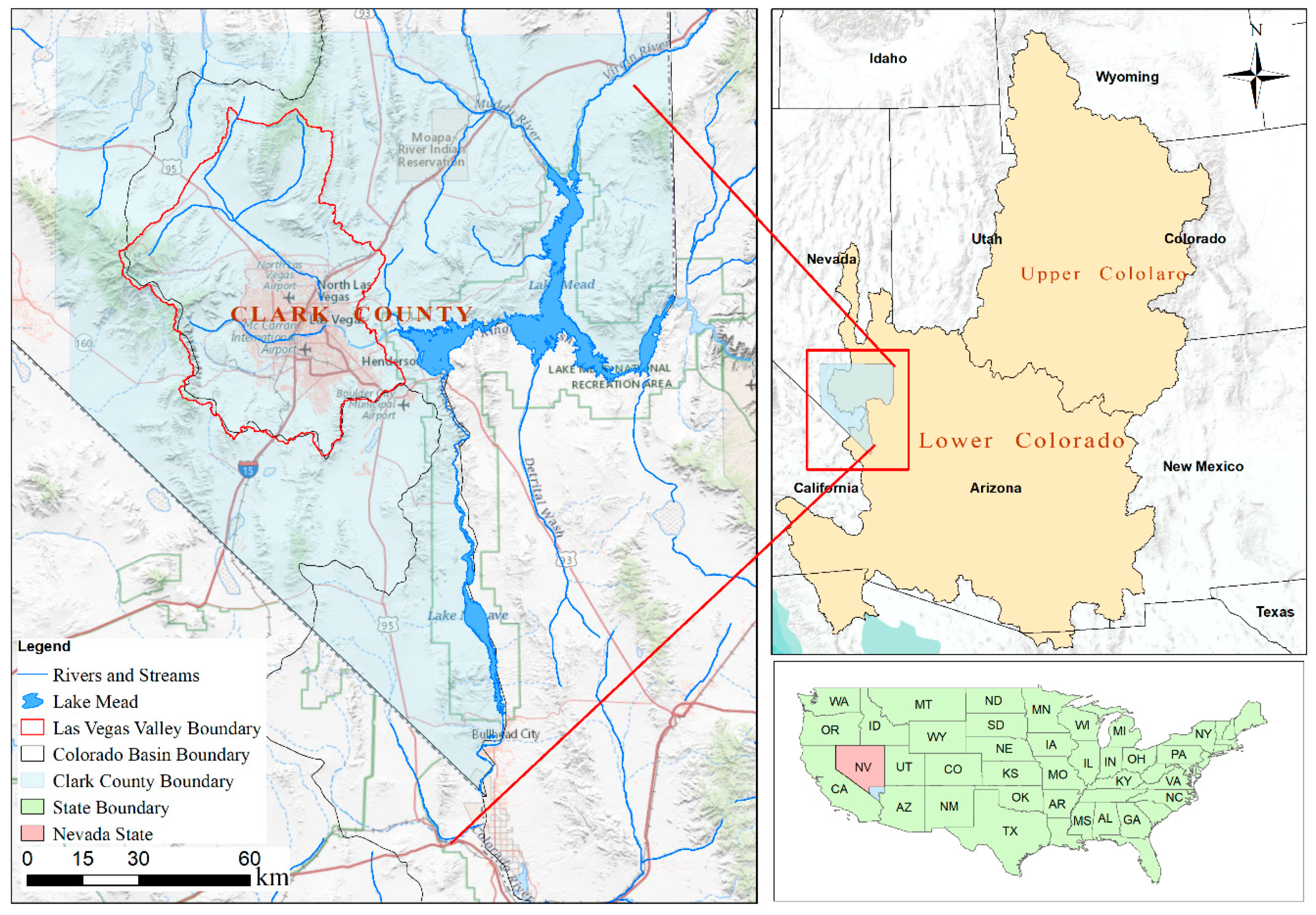
SD is a feedback-based dynamic problem addressing approach applied for complex systems [32,33,34]. It has been widely used in various environmental problems as well as to address water management issues [35,36]. SD modeling approach attributes to different components, creating a network system in terms of stocks and flows. Stocks and flows produce effects through feedback loops and represent system properties. The system’s performance may be altered, as it may have delayed response and internal feedback loops [34]. For example, feedback occurs between change in volume of reservoir water storage and evaporative losses as a function of volume/surface area of the reservoir. Stave [37] used SD modeling to incorporate participation from several stakeholders for water resources management. Qaiser et al. [38] studied the impact of water conservation practices on the outdoor water demand using SD modeling approach. Ahmad and Prashar [39] used SD modeling in South Florida to evaluate the relationship between municipal water availability and water demand. Dawadi and Ahmad [18] used an SD model to determine the impact of future climate change on the Colorado River flow. Using an SD model, Dawadi and Ahmad [40] studied the effect of demand-side water management in the LVV with respect to future climate change and population growth. Studies such as those of Qaiser et al. [38], Shrestha et al. [33], and Stave [37] have also focused on the supply and demand sides of water management; however, these studies did not consider the effects of climate change.

The current study considers the impacts of climate change by incorporating hydrological projections obtained from the Coupled Model Intercomparison Project phases 3 and 5 ensembles (CMIP3 and CMIP5, respectively), which are based on variable infiltration capacity (VIC) hydrologic model [41]. Bias-corrected spatial disaggregation projections from 16 GCMs of the CMIP3 model ensembles with three greenhouse gas emission scenarios were used, while 31 GCMs of the CMIP5 model ensemble with four representative concentration pathways (RCPs) were used in the analyses. Dawadi and Ahmad [18,40] also assessed the effects of climate change on supply and demand sides by using CMIP3 projections of temperature and precipitation from 16 GCMs with three emission scenarios and predicted Colorado River flow to decrease by about 3% until 2035. The current study assessed the future water supply conditions by incorporating population growth with climate change scenarios. The novelty of this study lies on the basis that it explored the advantage of the relatively recent simulations from the CMIP5 results and compared the future scenarios with the CMIP3 results. The results of the study may be helpful to foresee the probable future water supply and water demand scenarios using several climate projections. This also provides a useful comparison to trace out the differences in the CMIP3 and CMIP5 results. Comparison of the future projections from both the CMIP3 to CMIP5 simulations in the CRB has been made in other studies as well [42,43]. The temperature and precipitation projection until 2050 in Central Asia have a larger range obtained from CMIP5 than CMIP3 ensembles [43]. Sun et al. [43] found improvements in CMIP5 models over CMIP3 models for temperature variations and attributed them to advancement in reproducing observed annual average shortwave cloud forcing in CMIP5. However, such comparative studies used temperature and precipitation data from the CMIP3 and CMIP5 model ensembles to obtain the future hydrological projections, which is limited to application in hydrology only. This study used climate and population projections to determine both the supply and demand sides, which may have a broader application in the regional water resources management. Existing water management practices have also been incorporated to obtain demand scenarios for the future. This may be helpful to policymakers to address water conservation practices to meet the future water demand in the coming decades for the LVV.

3. Study Area

The LVV is one of the fastest-growing metropolitan cities in the U.S. and is located in Clark County, Nevada. Clark County has a population of 2,147,641 as of 2015 [44], and the valley is the most densely populated area in the county, with more than 90% of its population dwelling within the valley itself. The valley has experienced rapid population growth in recent times—growing from around 0.75 million to more than 2 million in a span of 25 years from 1990 to 2015. The daily average high (low) temperature is 38 °C (21 °C) and the valley has a very low relative humidity [45]. The average annual precipitation in the valley is only 4.5 inches. The major source of water is Lake Mead, which obtains water from the Colorado River. Ninety percent of the supply is met through the Colorado River and the remaining 10% of the supply is met from groundwater wells [46]. The valley is a major destination for tourists and receives around 40 million visitors annually. Figure 1 shows the location of the LVV with Lake Mead within the CRB.

SNWA is the main water management authority responsible for maintaining the supply and demand of the area. Since its inception in 1991, water conservation has been the major goal of SNWA. SNWA developed its first Water Resource Plan back in 1996. Even though significant progress has been made in water conservation practices, the water level of Lake Mead (the major water provider to SNWA) has dropped by more than 37 meters since January 2000, and its storage has been reduced to less than half of its capacity [47]. This can be attributed largely to the worst drought that has hit the Western U.S. during the first decade of the 21st century. To manage drought and ensure continuous water supply to its population, SNWA launched successful drought plan in 2003. During its first year, a whopping 23.1% savings was achieved [47]. Due to the climatic change and increased population, both hard path solutions and soft path solutions have been applied by SNWA to meet water use requirement. Water conservation practices by SNWA have led to the reduction of water demand from 1192 liters per capita per day (lpcd), which is equivalent to 315 gallons per capita per day (gpcd), in 2000 to 829 lpcd (219 gpcd) by the year of 2012, despite a more than 42% increase in the population during the same period [36]. In 2004, the goal of reducing water demand to 946 lpcd (250 gpcd) by 2010 was set, which was achieved two years ahead of schedule in 2008. SNWA has set a conservation goal of 753 lpcd (199 gpcd) for 2035 in 2009.

4. Materials and Methods

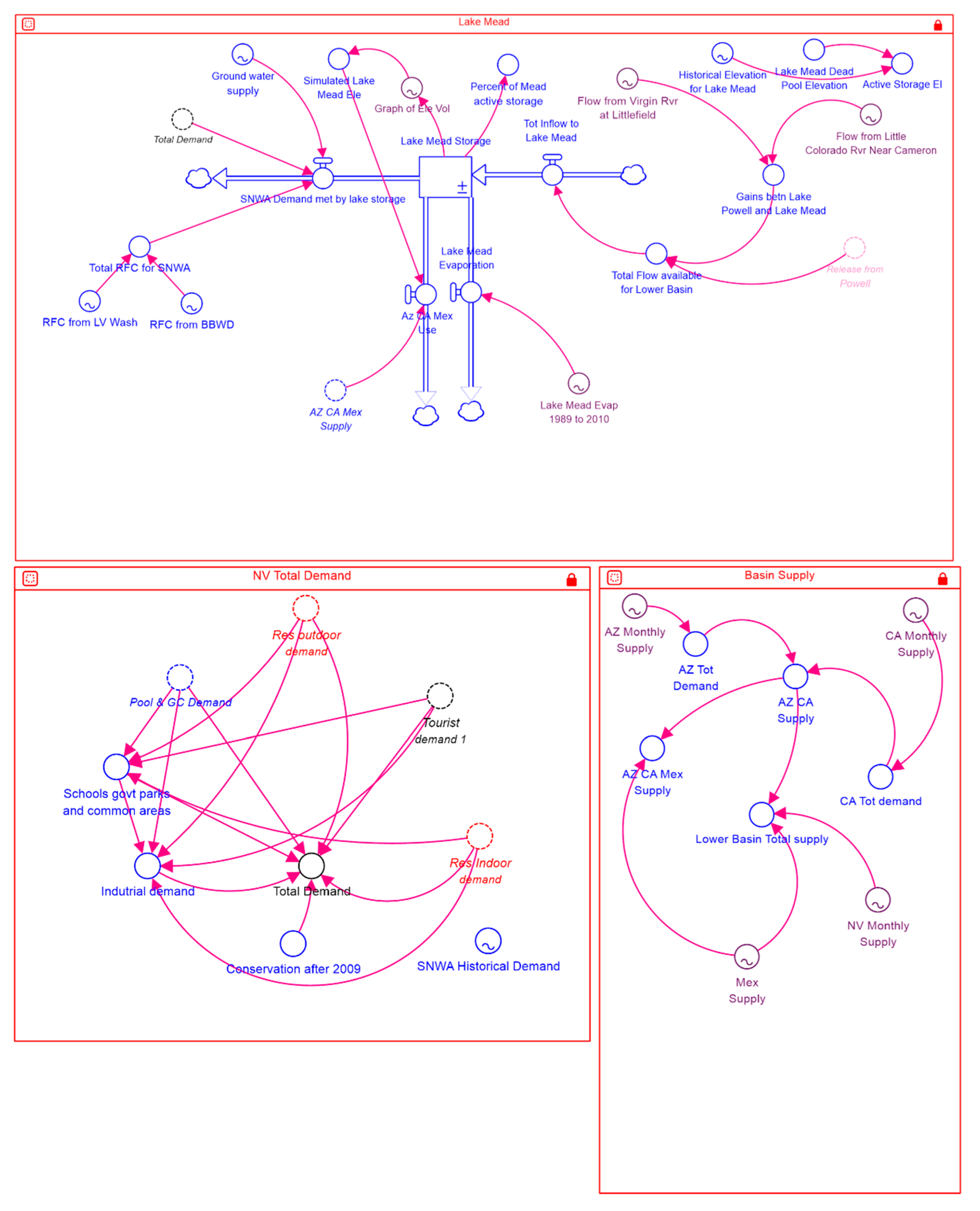
4.1. Modeling

To evaluate the effects of climate change and the growing population on the water supply and demand sides of the LVV, this study adopted SD modeling approach, which is a feedback-based system operation modeling technique with the inclusion of establishing relationships between stocks and flows using connectors and equations between several variables [34,48,49]. SD was applied using STELLA, a widely used system dynamics software. In STELLA, the model was simulated from 1989 to 2049 with 1989 to 2012 as a historical period and 2013 to 2049 as the future period with monthly time increment.

The model framework to simulate the effect of population, climate change, and conservation policies in the LVV was developed as shown in Figure 2. The model structure was primarily divided into four sectors: (1) Climate and Hydrological Projections Data Sector; (2) Lake Powell Operation Sector; (3) Lake Mead Operation with SNWA Supply Sector; (4) Demand Sector.

4.1.1. Climate and Hydrological Projections Data Sector

This sector provided the streamflow projections at Lees Ferry and temperature projections in the LVV for the different GCMs with their respective emission scenarios. Sixteen GCMs with three emission scenarios were used for the CMIP3 model ensemble and 31 climate models with four RCPs (based on their availability) were used for the CMIP5 model ensemble. A total of 48 (97) hydrological projections for the CMIP3 (CMIP5) model ensembles were analyzed in the study. Arrayed data were fed for each of the GCMs with each of the scenarios. GCMs and their scenarios could be changed to specify different inputs with the use of slider and knob in STELLA. Every unique GCM and unique scenario selection through knob and slider presented data for that GCM with its respective scenario.

4.1.2. Lake Powell Operation Sector

Historical naturalized streamflow at Lees Ferry for the historical period and the projected streamflow at Lees Ferry generated by the climate and hydrological projections for the future period were used as the inflow to Lake Powell operation sector. This sector was used to generate release to Lake Mead considering the upper basin consumptive uses and losses along with the evaporation loss from Lake Powell itself. Due to the absence of a naturalized streamflow gauge station at Lake Powell inlet, the naturalized streamflow at Lees Ferry was considered to have natural inflow to Lake Powell. Regulation criteria for releasing water from UCRB to LCRB were followed as per the reservoir guidelines. The two key criteria considered for Lake Powell operation were:

• A mandatory lower basin and Mexico release of 10.2 BCM/year [50,51]: Mandatory annual release was converted to the monthly release by using the conversion factor provided by U.S. Bureau of Reclamation (USBR) [52] and Dawadi and Ahmad [18].
• Equalization of Lake Mead and Lake Powell based on active storage of both reservoirs: An additional release for the LCRB above the mandatory release was provided if the available storage was found to be enough after equalization. An additional release was limited to 11.1 BCM/year. The percentage in the volume of Lake Mead and Lake Powell was equalized at each simulation month.

Lake Powell elevation data with respect to storage volume were used to generate simulated historical and future elevation.

4.1.3. Lake Mead Operation with SNWA Supply Sector

Lake Mead storage was considered as a stock for this sector. The release from Lake Powell, obtained from Lake Powell operation sector, and flows from major tributaries, namely Virgin River (USGS 09415000) at Littlefield and Little Colorado River (USGS 09402000) near Cameron in between Lake Powell and Lake Mead, were considered as inflows to the Lake Mead storage. The monthly historical flow data from 1989 to 2012 of these tributaries were obtained from the United States Geological Survey (USGS) gauging station at the confluence of those rivers with the Colorado River between Lake Mead and Lake Powell. Lake Mead feeds into the following lower basin states: California (CA), Arizona (AZ), Nevada (NV) and Mexico. Curtailment criteria below scheduled deliveries to the lower basin states from Lake Mead were based on those of the USBR [53].

In this operation sector, three different outflows from Lake Mead storage stock, namely Lake Mead evaporation, supply to lower basin states besides NV (AZ, CA, and Mexico), and water demand for NV obtained from Lake Mead, were considered. The water demand for NV to be fulfilled by Lake Mead storage was obtained by deducting groundwater supply and the total Return Flow Credits (RFC) obtained from SNWA from the total water demand in NV. The total water demand for NV was considered to be the same as the LVV within Clark County, which is under the jurisdiction of SNWA. This total water demand in the LVV was obtained from the Demand Sector. Lake Mead elevation against the storage data was used to obtain historical and future simulated elevation in the developed model. For this study, the demand for CA, AZ, and Mexico was assumed to remain constant for the future period after 2012.

4.1.4. Demand Sector

The total water demand in the LVV was evaluated in this sector. The demand included residential indoor demand, residential outdoor demand, tourist demand, swimming pool demand, golf course demand, and others as briefly described in the Appendix A.

4.2. Model Calibration and Validation

The primary objective of this study, as mentioned earlier, was to assess the water supply and demand sides of the LVV affected by climate change and population growth. Supply referred to the water storage in Lake Mead, which is the main source of supply for the valley, whereas the demand side referred to the total water demand in the valley. The water storage in Lake Mead is directly related to Lake Mead elevation, hence the latter rendered the supply. Therefore, the supply and demand evaluated in the model were Lake Mead elevation and the total water demand in the LVV, respectively.

The model was calibrated for both Lake Mead elevation and the total water demand for the historical period of 1989 to 2000. The parameter used to calibrate lake elevation included unaccounted flows to Lake Mead, while demand calibration included miscellaneous demands in the valley. Unaccounted flows referred to flows from small rivers, streams, or any other unknown flows, and miscellaneous demands in the LVV included demands not accounted hereupon. Careful selection of these parameters was considered, while only a small percentage of either the total flow or total demand was used to calibrate the model. Manual calibration was carried out in the study, and the aforementioned parameters were adjusted to get a close match between the simulated and observed dataset. Bias-corrected GCM outputs were used for temperature and precipitation, which reduces a certain level of uncertainty. The performance of the calibrated model was quantified by using different statistical indices like root-mean-square error (RMSE), RMSE-observations standard deviation ratio (RSR), percent bias (PBIAS), Nash Sutcliffe coefficient (NSE), correlation coefficient (r), and coefficient of determination (R²) for the historical period of 1989 to 2000. The developed model was validated for Lake Mead elevation and the total water demand for a 12-year period (2001 to 2012) using the performance indices.

4.3. Future Simulation

The future simulations for Lake Mead elevation and the total water demand spanned from 2013 to 2049 in monthly time steps. Future streamflow of the Colorado River and future temperature in the LVV (as predicted by various projection scenarios) were used as climate factors affecting the future supply and demand. Population forecasts from Centre for Business and Economic Research (CBER) [54] were used as another influencing factor for future simulations. Conservation policies, such as outdoor conservation, indoor conservation, and Price Elasticity of Demand (PED) effect, were also considered.

4.4. Evaluation of Model Performance

The model performance of Lake Mead under several scenarios was evaluated on the basis of reliability. Water supply system from Lake Mead to LVV can be considered reliable if lake level remains above 327.7 m (1075 ft). Below this level, it triggers the shortage criteria in Nevada. Reliability of this supply system was calculated for each climate model and their respective emission scenarios for the future period. The simulated mean lake level below 327.7 m (1075 ft) over a month was considered as the magnitude of failure. Hence, reliability for each of the projection scenarios from both the CMIP3 and CMIP5 model ensembles was obtained using the total number of successful (as opposed to failure) months over the future period. Mean reliability for each of the emission scenarios was also calculated.

4.5. Reliability Analysis

Reliability provides an index of the system’s capacity to meet anticipated water demand. In other words, high reliability refers to less variability [55]. The reliability model is a widely used index for risk analysis. Reliability is defined by “how often a certain level of demand is met or a volume of reservoir storage is maintained”. Resilience is defined by “how long a demand is not met or the volume of storage is not maintained”, and vulnerability is defined by “how much demand was short or how far the volume of storage goes below the desired level”. The main aim of the current study was to check the variability of a water system. The reliability of a system is altered by variability and availability of water supply, as well as population demand volume and variability. Water storage serves as a safeguard to supply and demand ratio, and hence reservoir storage levels can be used as an indicator of the water system’s performance and system’s capability to meet anticipated demands [56]. The assessment of water level is an appropriate measure to evaluate performance and risk associated with the water system. The reliability index is suitable to evaluate the acceptable level of risk and level of service as well as to modify the reliability goal of allowing implementation of shortage response measures. It is helpful to mitigate unforeseen events by calculating the water deficit and allocating emergency storage (risk mitigation). In addition, shortage response measures can also be taken by considering the normal water level (risk management), if exceeded during certain years as a management strategy, as well as to check the achieved indoor water demands.

The aforementioned water resources risk management plans were considered as an objective of this study and reliability analysis was used to assess the performance of the water system to meet the demand. Reliability, the average duration of failure, number of failures, and the average deficit were calculated. Reliability is calculated using the following formula from Zongxue et al. [57] as shown below.

$$\mathrm{Reliability}=\frac{1}{\mathrm{NS}}{\displaystyle \sum }_{\mathrm{i}=1}^{\mathrm{NS}}{\mathrm{I}}_{\mathrm{i}}$$

(1)

where, NS is the total duration of water supply and I_i is the state variable of the water supply system.

The average duration of failure was calculated as the sum of the duration of failures divided by the number of failures. Similarly, the average deficit as a percentage of demand was calculated by dividing the sum of all deficits during the water supply period by the water demand during the deficit period; this value increases with the increase in water deficit. Reliability is equal to 1 if there is no deficit and is equal to 0 if there is a deficit.

5. Data and Model Simulations

Datasets used in this study included downscaled climate and hydrological projections (modeled outputs), reservoir data, water supply data for the basin states, naturalized runoff data, population data, and others (as shown in

Table 1. Data used in the study and their sources.

SN	Data	Source
1	Climate and Hydrological Projections Data	Downscaled CMIP3 and CMIP5 Climate and Hydrology Projections [58]
2	Reservoir Data for Lake Powell and Lake Mead	US Department of Interior (USDOI) Bureau of Reclamation [59,60]
3	Basin States Water Use Data for Colorado River	USDOI Bureau of Reclamation [61]
4	Naturalized Streamflow Data	USBR [62]
5	Resident Population Data	SNWA [47]
6	Tourist Population Data in Las Vegas	Las Vegas Convention and Visitors Authority (LVCVA) [63]
7	No. of Houses Data in Clark County	Clark County Comprehensive Planning Department (CCCPD)
8	Turf Area in LVV	SNWA [46]
9	Swimming Pool Area in LVV and Conservation by Pool Covers	Sovocol and Morgan [64], SNWA [47]
10	Golf Course Area in LVV	Clark County Nevada (CCN) [65]
11	Price Elasticity of Demand in LVV	SNWA [47]
12	Groundwater Supply Data	SNWA [16]
13	Return Flow Credits Data	SNWA [16]
14	Flow Data for Virgin River and Little Colorado River	USBR [66]
15	Guidelines for Curtailment to Lower Basin States	USDOI [53]

). The study period spanned from 1989 to 2049. Datasets from 1989 to 2012 were considered as historical data, while the climate and hydrological projections and the population forecasts from 2013 to 2049 were analyzed as the future data. The data used in this study along with their sources are listed in Table 1.

5.1. Climate and Hydrological Model Outputs

The study used climate and hydrological model outputs from both the BCSD-CMIP3 and BCSD-CMIP5 model ensembles from 1950 to 2099. Between the two available data resolutions—1/8° latitude–longitude and 2° latitude-longitude—data with a spatial resolution of 1/8° latitude–longitude were used. Climate model outputs used for this study refer to the temperature projections of the model ensembles for the LVV, whereas the hydrological data refer to the streamflow projections of the model ensembles at Lees Ferry on the Colorado River.

There were 16 GCMs altogether in the CMIP3 model ensembles with three emission scenarios, namely A1b, A2, and B1. The emission scenarios are based on the CO₂ emission concentrations in the atmosphere. Similarly, there were 31 GCMs in the CMIP5 model ensembles with four RCPs (RCP2.6, RCP4.5, RCP6, and RCP8.5). RCPs are greenhouse gas (GHG) concentration trajectories used by the Intergovernmental Panel on Climate Change AR5. They are considered based on how much GHGs are emitted. Monthly climate projection outputs, in the form of projected average surface air temperature, from four RCPs of the CMIP5 ensembles, were used in the study. With the CMIP3 ensembles, monthly climate projections (as average surface air temperature) of all the climate models with three emission scenarios in the LVV were considered. Similarly, monthly hydrological projections, in the form of projected streamflow at Lees Ferry, of all the climate models with their respective emission scenarios for both the CMIP3 and CMIP5 ensembles were used. Streamflow data were available in cfs (35.31 cfs = 1 m³/s), while temperature data were obtained in °C. There were a total of 112 climate and hydrological projections available from the CMIP3 model ensembles, while a total of 234 climate projections and 97 hydrological projections [41,67] were available from the CMIP5 model ensembles. This study considers a single simulated future per climate model per scenario (16 GCMs × 3 emission scenarios or 31 GCMs × 4 emission scenarios for CMIP3 and CMIP5, respectively)—even though some of the GCMs had up to five simulations per emission scenario.

5.2. Reservoir Data

Reservoir data for Lake Mead and Lake Powell were obtained from the USBR [59,60] online database. Data for Lake Mead were available from 1934 to 2016, while data for Lake Powell were available from 1963 to 2016. Average storage, average elevation, average evaporation, and average inflow and outflow for each of the month were extracted from 1989 to 2012. Elevation data were obtained in ft (1 ft = 0.3048 m), while storage, flow, and evaporation data were obtained in ac-ft (1 ac-ft = 1233.48 m³). Graphical relationship between mean storage and mean elevation were used to simulate the developed model.

5.3. Basin State Water Use Data

Historical water usage data for the UCRB for each of the upper basin states were obtained from the UCRB Consumptive Uses and Losses Report [61]. The withdrawal data for the LCRB for each of the lower basin states were obtained from the LCRB Water Accounting Report [68]. The data were available in ac-ft. Monthly historical data from 1989 to 2012 was used for the study.

5.4. Naturalized Stream Runoff

To study the impact of climate change, monthly streamflow data (in cfs), which were not affected by human interventions, were obtained from USBR [62] for the stream gauge station located at Lees Ferry on the Colorado River for the period 1989 to 2012. USBR has prepared the data by adjusting the human factors (e.g.; reservoir regulation and other consumptive uses like irrigation, municipal and industrial use, and evaporation) that affect streamflow.

5.5. Population Data

Population data for Southern Nevada, which is under the jurisdiction of SNWA, were used in the study. Yearly population data from 1989 to 2012 were obtained from SNWA [47]. The population during the whole period of a year was assumed to remain the same due to lack of monthly population data. The total resident population dependent upon SNWA for water was about 1.945 million in 2012. Tourist population for each year from 1989 to 2012 was obtained from the LVCVA [63]. Tourist population data for a month were taken the same throughout a year. Visitors’ population for 2012 was approximately 39.73 million. Houses data on a monthly scale from the period of 1989 to 2012 were obtained from the CCCPD. Predicted future resident population data from 2013 to 2049 were obtained from the CBER, University of Nevada, Las Vegas [54]. Tourists’ population and the number of houses were assumed to increase at the same rate as the resident population. For the forecasts, data were available on a yearly scale; for simplicity, data for each month were considered to be the same for a particular year.

5.6. Other Data

The total turf area in the LVV was obtained from SNWA [46]. The swimming pool area in the valley and water conservation through pool covering were obtained from Sovocool and Morgan [51]. Golf course area was obtained from the Clark County Nevada [65] online database. PED was obtained from SNWA [47]. Groundwater supply data and RFC data were obtained from SNWA [16]. Streamflow data for the Virgin River and Little Colorado River were obtained from USBR [66].

6. Results

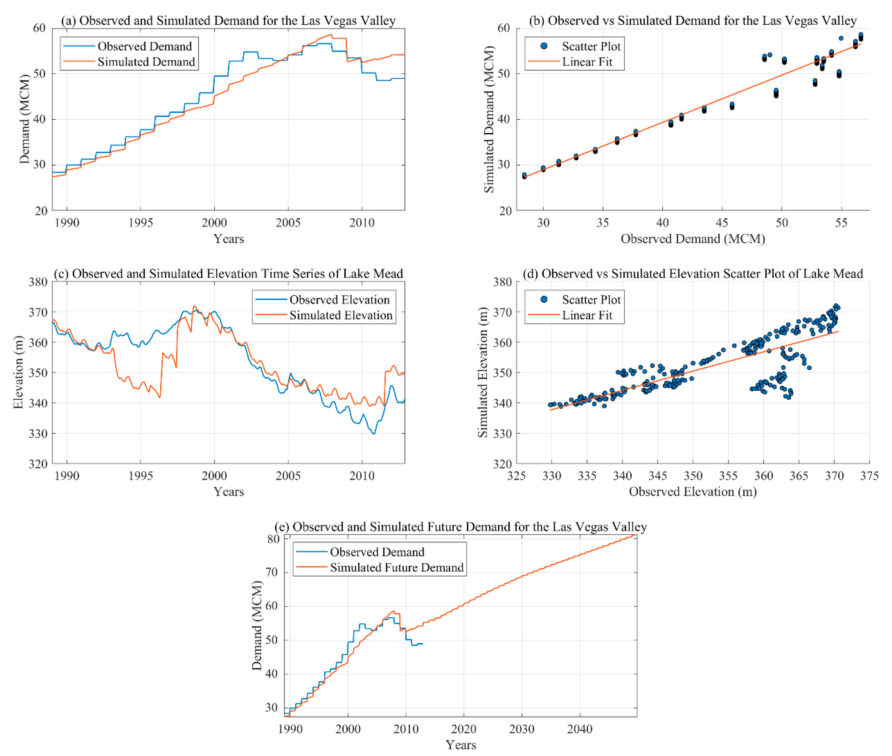
6.1. Model Validation

The modelling approach consisted of model validation and future simulation. The model performance was evaluated based on the total water demand in the LVV and Lake Mead elevation. The model performed satisfactorily under all statistical indices. The model was validated for water demand in the LVV from 2001 to 2012 and calibrated for both Lake Mead elevation and the total water demand for the historical period of 1989 to 2000.

6.1.1. Total Water Demand

A graphical comparison between observed and simulated water demand is shown in Figure 3a. The R² value of 0.97 was found between the observed and simulated water demand, as shown in Figure 3b. In the first two-thirds of the historical period of the study, the model predicted relatively closely to the observed values. However, the simulated values were found higher than the observed values during the latter part of the study period. This might be due to SNWA’s strict implementation of conservation policies after 2000, which resulted in reduced demand. Moreover, conservation programs were more stringent after 2009. The values of the performance measures, namely, RSR, PBIAS, and NSE were found to be 0.17, 0.99%, and 0.95, respectively, which were found to be within the satisfactory range as suggested by Moriasi et al. [69].

6.1.2. Lake Mead Elevation

Figure 3c shows the observed and simulated lake elevations over the historical period of the study. The simulated elevations predicted by the model suggested a satisfactory correlation with the observed elevations, as shown in Figure 3d. The model predicted quite appropriately during the latter half of the study, which was considered very important, especially for the drought period after 2000. Overall, the model had a satisfactory performance with a correlation coefficient of 0.8, an RSR of 0.6, and a PBIAS of 0.24%.

6.2. Future Simulation

6.2.1. Total Water Demand

Historical and simulated water demand for the historic and future periods, respectively, are presented in Figure 3e. As water demand for the future period will be predominantly governed by the population growth (based on the developed model), the slope of the demand curve gradually but consistently decreased in the long-term future, as depicted in the figure. During the first eighteen years of the study period (2013 to 2048), water demand increased by 24.9%, while during the last eighteen years it increased by 16.4%. The monthly water demand at the end of 2049 was found to be 81 Million Cubic Meters (MCM) (65,857 ac-ft), while the annual demand was 972 MCM (788,822 ac-ft) at the end of 2049 in LVV. This demand was evaluated considering all the conservation policies specified in the methodology section.

SNWA conservation goal for 2035 corresponded to 753 lpcd (199 gpcd) [46], which is equivalent to 894 MCM (725,000 ac-ft) for the year 2035, whereas the total water demand obtained from this study for the year 2035 was about 869 MCM (704,562 ac-ft). Similarly, the demand predicted by SNWA for the year 2049 was 1011 MCM (820,000 ac-ft). The current study predicted the demand to be around 972 MCM (788,823 ac-ft). This suggests that the result from the current model slightly underestimates the long-term demand as compared to SNWA. With the conservation programs implemented as assumed hereupon, the results of this study conclude that SNWA will be able to achieve their goal.

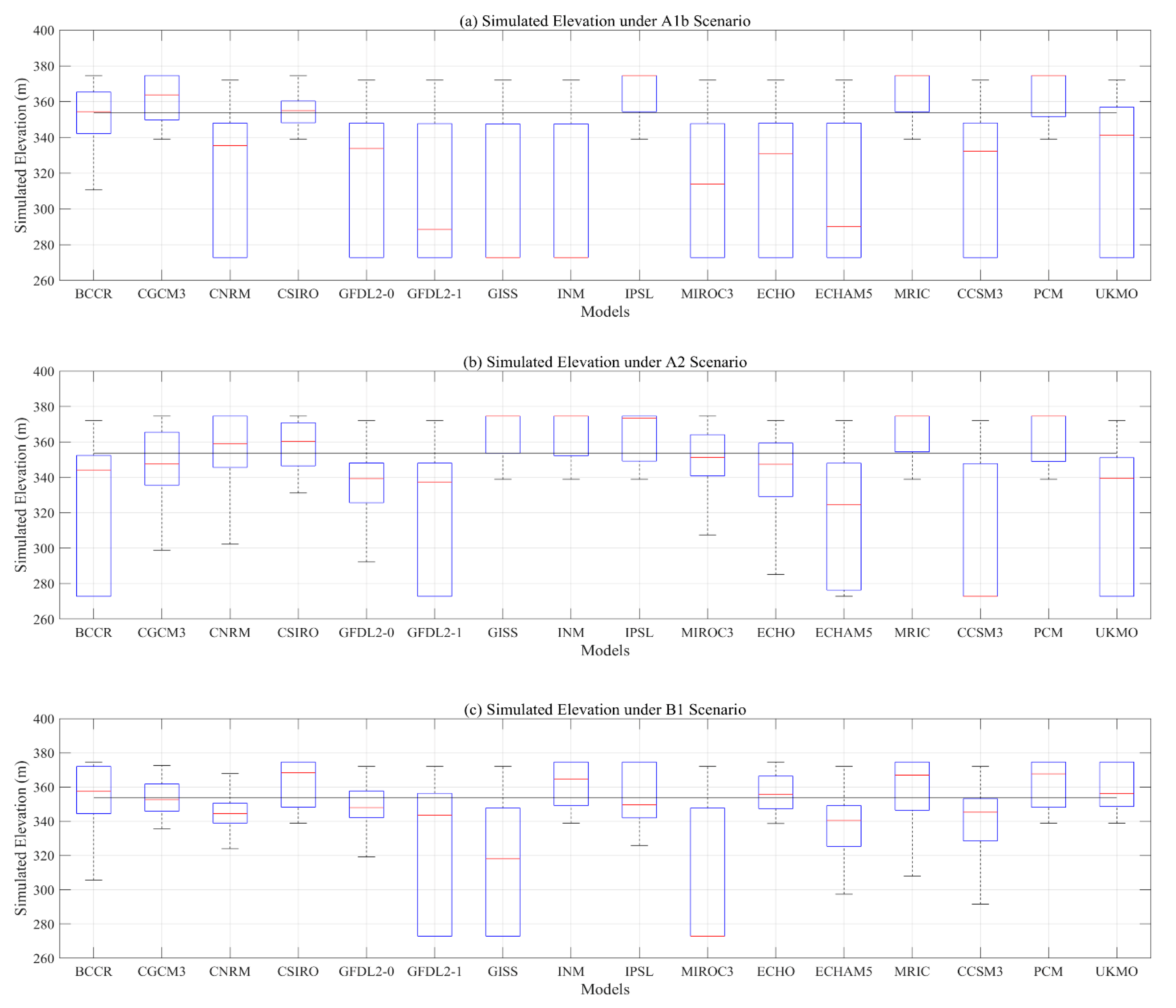
6.2.2. Lake Mead Elevation

Computation of Lake Mead elevation was carried out in order to obtain future water supply scenarios in LVV. Mean monthly elevation from January 2013 to December 2049 was obtained using 48 (97) hydrological projections from the CMIP3 (CMIP5) model ensembles with streamflow at Lees Ferry as the major flow input. The future elevation was obtained on the basis that the major outflow from Lake Mead to LVV corresponds to the total water demand in the valley, which was obtained separately for the future period (using the sector explained above). All conservation programs considered for water demand management were assumed to be implemented in the future. Observed mean lake elevation for the historical period (1989 to 2012) was calculated from the available mean monthly historical data from USBR, and it was found to be 1160.3 m. Simulated mean lake elevation for the future period from 2013 to 2049 was computed for all the models and their respective emission scenarios. Percentage change in Lake Mead elevation for the future period from the historical period was calculated for different climate models and their respective emission scenarios.

Table 2. Simulated future mean Lake Mead elevation (2013-2049) and its deviation from the observed historical mean (1989-2012) for the Coupled Model Intercomparison Project phase 3 (CMIP3) simulation models and their respective emission scenarios.

WCRP CMIP3 Climate Model ID	A1b		A2		B1
	Simulated Future Mean Lake Mead Elevation (m)	Change from the Observed Historical Mean Lake Mead Elevation (%)	Simulated Future Mean Lake Mead Elevation (m)	Change from the Observed Historical Mean Lake Mead Elevation (%)	Simulated Future Mean Lake Mead Elevation (m)	Change from the Observed Historical Mean Lake Mead Elevation (%)
BCCR-BCM2.0	337.20	−4.70	308.43	−12.8	354.27	0.20
CGCM3.1 (T47)	367.92	4.00	344.12	−2.70	354.42	0.20
CNRM-CM3	288.46	−18.4	360.09	1.80	340.22	−3.80
CSIRO-Mk3.0	356.10	0.70	362.77	2.60	368.84	4.30
GFDL-CM2.0	295.23	−16.5	316.44	−10.5	341.19	−3.50
GFDL-CM2.1	282.49	−20.1	303.76	−14.1	299.86	−15.2
GISS-ER	276.67	−21.8	372.98	5.50	297.61	−15.8
INM-CM3.0	276.67	−21.8	372.56	5.30	367.86	4.00
IPSL-CM4	373.14	5.50	370.00	4.60	353.96	0.10
MIROC3.2	290.02	−18.0	332.63	−6.00	281.39	−20.4
ECHO-G	292.85	−17.2	328.21	−7.20	359.85	1.70
ECHAM5/MPI-OM	282.24	−20.2	297.58	−15.9	326.20	−7.80
MRI-CGCM2.3.2	373.26	5.50	373.50	5.60	363.53	2.80
CCSM3	291.39	−17.6	281.33	−20.5	319.92	−9.50
PCM	372.19	5.20	370.12	4.70	368.44	4.20
UKMO-HadCM3	299.07	−15.4	294.99	−16.6	362.96	2.60

provides simulated future mean Lake Mead elevation and its percentage deviation from the observed historical mean for the CMIP3 model ensembles and the three emission scenarios—A1b, A2, and B1.

Table 3. Simulated future mean Lake Mead elevation (2013–2049) and its deviation from the observed historical mean (1989–2012) for the Coupled Model Intercomparison Project phase 5 (CMIP5) simulation models and their respective representative concentration pathways (RCPs).

WCRP CMIP5 Climate Model ID	Representative Concentration Pathways (RCPs)
	RCP 2.6		RCP 4.5		RCP 6.0		RCP 8.5
	Simulated Mean Elevation (m)	% Change	Simulated Mean Elevation (m)	% Change	Simulated Mean Elevation (m)	% Change	Simulated Mean Elevation (m)	% Change
ACCESS1-0	-	-	288.52	−18.4	-	-	288.01	−18.6
BCC-CSM1-1	276.67	−21.8	370.70	4.8	276.67	−21.8	363.50	2.8
BCC-CSM1-1-M	-	-	295.14	−16.5	-	-	283.95	−19.7
CanESM2	353.81	0.0	337.41	−4.6	-	-	335.92	−5.0
CCSM4	278.98	−21.1	310.32	−12.3	315.50	−10.8	361.83	2.3
CESM1-BGC	-	-	319.28	−9.7	-	-	296.39	−16.2
CESM1-CAM5	367.44	3.9	372.34	5.3	317.36	−10.3	306.48	−13.3
CMCC-CM	-	-	323.48	−8.5	-	-	281.82	−20.3
CNRM-CM5	-	-	371.52	5.0	-	-	372.40	5.3
CSIRO-Mk3-6-0	308.03	−12.9	290.81	−17.8	295.05	−16.6	290.72	−17.8
FGOALS-g2	367.83	4.0	349.33	−1.2	-	-	345.58	−2.3
FIO-ESM	284.38	−19.6	359.05	1.5	326.01	−7.8	295.93	−16.3
GFDL-CM3	368.50	4.2	348.23	−1.5	296.78	−16.1	344.15	−2.7
GFDL-ESM2G	331.84	−6.2	332.38	−6.0	372.83	5.4	371.43	5.0
GFDL-ESM2M	360.12	1.8	372.25	5.3	341.44	−3.5	368.17	4.1
GISS-E2-H-CC	-	-	-	-	371.80	5.1	-	-
GISS-E2-R	-	-	-	-	372.68	5.4	-	-
GISS-E2-R-CC	313.73	−11.3	366.00	3.5	361.74	2.3	371.49	5.0
HadGEM2-AO	299.71	−15.3	286.54	−19.0	293.71	−17.0	285.81	−19.2
HadGEM2-CC	-	-	308.88	−12.7	-	-	308.88	−12.7
HadGEM2-ES	285.05	−19.4	306.38	−13.4	299.59	−15.3	331.38	−6.3
INM-CM4	-	-	366.19	3.5	-	-	359.85	1.8
IPSL-CM5A-MR	373.23	5.5	370.09	4.6	363.72	2.8	357.44	1.1
IPSL-CM5B-LR	-	-	315.83	−10.7	-	-	362.89	2.6
MIROC-ESM	368.99	4.3	371.46	5.0	370.36	4.7	364.24	3.0
MIROC-ESMCHEM	352.50	−0.3	292.27	-17.4	367.74	4.0	347.41	−1.8
MIROC5	368.26	4.1	288.86	−18.3	329.31	−6.9	368.23	4.1
MPI-ESM-LR	297.33	−15.9	-	-	277.95	−21.4	315.22	−10.9
MPI-ESM-MR	371.92	5.2	347.01	−1.9	-	-	372.53	5.3
MRI-CGCM3	351.92	−0.5	315.89	−10.7	-	-	302.70	−14.4
NorESM1-M	325.40	−8.0	323.15	−8.6	288.31	−18.5	357.90	1.2

tabulates simulated future mean Lake Mead elevation and its percentage deviation from observed historical mean for the CMIP5 model ensembles and the four RCPs—RCP 2.5, RCP 4.5, RCP 6.0, and RCP 8.5. The assigned negative sign shown in the table indicates a drop in lake elevation in the future, whereas a positive sign indicates a rise in lake elevation. Out of the total 48 climate and hydrological projections from the CMIP3 model ensembles, 27 projections, i.e.; more than 55%, predicted that the mean lake level would be lower in the future compared to the historical period. More noticeably, 16 out of the 27 projections predicted that the future simulated mean lake level would be lower than the observed historical mean level by 15% or more. The climate model INM-CM3.0, under the A1b scenario, predicted the highest deviation of -21.8% from the historical mean. The models predicting a rise in lake level in the future from the historical mean showed no more than 5.6% increment (this value was obtained from the model MRI-CGCM2.3.2 under the A2 scenario). Similarly, out of the total of 97 climate and hydrological projections from the CMIP5 model ensembles, 59 projections (60% of total projections) indicated that the lake level would drop in the future. Among these 59 projections, 26 projections indicated that the future simulated mean level would be lower by 15% or more than the historical mean level. BCC-CSM1-1 for RCP 2.6 predicted the highest drop of −21.8%. Climate model IPSL-CM5A-MR under RCP 2.6 predicted the highest rise of 5.5%.

Boxplots of future simulated Lake Mead elevation (from January 2013 to December 2049) for the CMIP3 and CMIP5 model ensembles are presented in Figure 4 and Figure 5, respectively. The solid black line indicates the mean of the observed historical lake elevation. Each boxplot shows the predicted future lake elevation variability with the associated model under the corresponding emission scenario. The upper and lower bounds represent the 25th and 75th percentiles, respectively. The solid horizontal red line within the box corresponds to the median and the whiskers at the lower and upper ends represent the 5th and 95th percentiles, respectively.

Some of the boxplots in each of the scenarios from the CMIP3 model ensembles indicated that Lake Mead elevation could go as low as 272.8 m (895 ft) (empty lake condition) and as high as 374.6 m (1229 ft) (full lake condition). Similar inference can be drawn from the boxplots in Figure 5 for the CMIP5 models. In Figure 4, under emission scenario A1b, most of the boxes were found to lie below the solid line (which represents the historical mean). This suggests that the future mean lake elevation for that emission scenario would be lower than the historical mean lake elevation for most of the climate models. Among the 16 climate models for this scenario, 10 predicted that Lake Mead will go completely dry. However, for the other two emission scenarios from the CMIP3 models, namely A2 and B1, almost half of the climate models predicted that the median of the future lake elevation would remain above the historical mean. Figure 5 shows that out of the 21 models under RCP 2.6, 11 models anticipated that the median value for the future elevation would remain below the historical elevation. Similarly, 20 out of 31 models under RCP 4.5, 11 out of 16 models under RCP 6.0, and 15 out of 31 models under RCP8.5 predicted that the median value for the future would remain below the historical mean. RCP 6.0 raised the potential risk of lake elevation going down in the future more than the others.

Presently, there is no guideline of supply curtailment from Lake Mead for the basin states when the lake level drops below 304.8 m (1000 ft) [53]. Hence, an indication of the level going below 304.8 m (1000 ft) would raise an alarm to the authorities. The results of the current study showed that 17 out of the 48 projections from the CMIP3 model ensembles predicted that the mean level would go below 304.8 m (1000 ft) in the future. Likewise, out of the 97 projections from the CMIP5 model ensembles, 27 indicated the mean level to go below 304.8 m (1000 ft).

6.3. Reliability

For the CMIP3 climate models, mean reliabilities of water supply system from Lake Mead to LVV during the future period for emission scenarios A1b, A2, and B1 were evaluated to be 0.45, 0.66, and 0.75, respectively. Similarly, for the CMIP5 climate models, mean reliabilities for RCP 2.6, RCP 4.5, RCP 6.0, and RCP 8.5 were 0.63, 0.62, 0.57, and 0.66, respectively. On average, close to two-thirds of the results were found to be reliable. The reliability results from the climate models of CMIP3 and CMIP5 along with their respective emission scenarios are presented in

Table 4. Mean reliabilities for the CMIP3 simulation models and their respective emission scenarios.

WCRP CMIP3 Climate Model ID	Reliability
	A1b	A2	B1
BCCR-BCM2.0	0.68	0.42	0.78
CGCM3.1 (T47)	1.00	0.68	1.00
CNRM-CM3	0.21	0.93	0.94
CSIRO-Mk3.0	1.00	1.00	1.00
GFDL-CM2.0	0.25	0.47	0.79
GFDL-CM2.1	0.09	0.34	0.31
GISS-ER	0.04	1.00	0.09
INM-CM3.0	0.04	1.00	1.00
IPSL-CM4	1.00	1.00	0.98
MIROC3.2	0.08	0.66	0.09
ECHO-G	0.22	0.60	1.00
ECHAM5/ MPI-OM	0.09	0.17	0.53
MRI-CGCM2.3.2	1.00	1.00	0.86
CCSM3	0.18	0.09	0.60
PCM	1.00	1.00	1.00
UKMO-HadCM3	0.31	0.24	1.00
Mean	0.45	0.66	0.75

and

Table 5. Mean reliabilities for the CMIP5 simulation models and their respective representative concentration pathways (RCPs).

WCRP CMIP5 Climate Model ID	Reliability
	RCP 2.6	RCP 4.5	RCP 6.0	RCP 8.5
ACCESS1-0	-	0.20	-	0.18
BCC-CSM1-1	-	0.25	-	0.10
BCC-CSM1-1-M	0.04	1.00	0.04	1.00
CanESM2	0.70	0.70	-	0.82
CCSM4	0.07	0.35	0.55	0.94
CESM1-BGC	-	0.46	-	0.28
CESM1-CAM5	1.00	1.00	0.34	0.28
CMCC-CM	-	0.70	-	0.11
CNRM-CM5	-	1.00	-	1.00
CSIRO-Mk3-6-0	0.45	0.22	0.11	0.20
FGOALS-g2	1.00	-	0.90	0.91
FIO-ESM	0.14	0.93	0.35	0.18
GFDL-CM3	1.00	0.73	0.20	0.74
GFDL-ESM2G	0.55	0.67	1.00	1.00
GFDL-ESM2M	1.00	1.00	0.70	1.00
GISS-E2-H-CC	-	1.00	-	-
GISS-E2-R	0.33	1.00	1.00	1.00
GISS-E2-R-CC	-	1.00	-	-
HadGEM2-AO	0.14	0.17	0.28	0.16
HadGEM2-CC	-	0.22	-	0.22
HadGEM2-ES	0.17	0.38	0.33	0.65
INM-CM4	-	1.00	-	0.95
IPSL-CM5A-MR	1.00	1.00	1.00	0.89
IPSL-CM5B-LR	-	0.36	-	1.00
MIROC-ESM	1.00	1.00	1.00	1.00
MIROC-ESMCHEM	0.96	0.24	1.00	0.98
MIROC5	1.00	0.17	0.63	1.00
MPI-ESM-LR	0.17	0.06	-	0.38
MPI-ESM-MR	1.00	0.89	-	1.00
MRI-CGCM3	1.00	0.48	-	0.31
NorESM1-M	0.49	0.51	0.20	0.89
Mean	0.63	0.62	0.57	0.66

, respectively.

7. Discussion

The results of the predicted future water demand suggested that SNWA can achieve its conservation goal only if the conservation programs are persistently implemented in the future. However, it is difficult to determine if such conservation programs will offer the same efficacy in the future. For example, indoor conservation may not result in a significant reduction in demand in the future since much of the indoor water use is already recycled and returned to the supply source through RFCs; hence, not much benefit can be made in terms of net conservation [70]. Moreover, after a certain rise in price, demand cannot be reduced further as all the potential to conserve water might already be exploited by then. Even outdoor conservation, which offers a greater savings opportunity than indoor conservation [70], cannot reduce the demand after a certain extent, as there will always be the need for minimum outdoor demand. Future water demand was also evaluated considering the future population growth. Even though the population is expected to rise in the future for LVV, this might not always be the case. The economic recession during the late 2000s resulted in a decrease in population in LVV. Hence, the economy might play an important role in what the future will hold for the population. Other factors that might affect population growth and this uncertainty in population growth may result in uncertainty in evaluating future demand.

LVV receives water from Lake Mead, but Lake Mead is also a supplier for AZ, CA, and Mexico. This study assumes that the demand for the other basin states and Mexico will remain constant, which may not be the case in the future. Though these states are already using most of their allocated budget of total supply, change in their demand pattern can lead to change in Lake Mead elevation, and the projected results from this study for future Lake Mead elevation may not hold true. Moreover, the supply curtailment criteria for basin states from Lake Mead may require revisions in the future due to a reduction in supply, and this would result in an entirely different scenario. Lake Mead is operated in coordination with Lake Powell, and change in the latter’s operation criteria may alter the predicted elevation of Lake Mead. Currently, no guidelines exist for supply curtailment to basin states when Lake Mead elevation drops below 304.8 m (1000 ft). Unfortunately, the probability of the lake drawing down below this elevation in the future cannot be discarded considering the recent prolonged drought. To address this worst possible scenario, SNWA has already established a third intake that can draw water even after the lake level drops below 304.8 m (1000 ft). In addition, a low-level pumping station is under installation that will draw water below 273.8 m (895 ft), the level at which Lake Mead ceases to release downstream. The introduction of any new guidelines for the operation of these new water-drawing systems would change the reliability of the supply system of Lake Mead to LVV.

Groundwater contribution to LVV, though not much significant, cannot be ignored. This study assumes a constant groundwater contribution and evaporation loss in the future due to the difficulty in assessing the future groundwater condition in LVV under the changing climate. However, this assumption cannot be entirely justified, especially for long-term decision making, as it has been shown by previous studies that the change in precipitation trends, changes in subsurface conditions, and many other factors severely affect the status of groundwater [71,72]. Rise in temperature due to climate change in the future will tend to increase evaporation loss, resulting in reduced storage.

GCMs have their own uncertainties and limitations [73]. The reliability of the results from the current study also depends upon the reliability of the use of GCMs. The uncertainties in the results can be minimized by using various climate projections [29,74]. The uncertainties could be from natural variability, nature of human behavior, and also may be in the model formulation while understanding the physical processes. This includes internal variability of climate systems, intermodel variability, and variability between emission scenarios. The integration of multiple models is a rational and well-accepted approach to address model uncertainty [75,76]. The model ensemble has less variability than using an individual model [77]. As suggested by Weigel et al. [78] and Hagedorn et al. [79], the multimodel ensemble improves reliability and reduces the uncertainty of climate projections and forecasting. For hydrological research, Gharbia et al. [80] suggested utilizing the multimodel ensemble for climate change simulations and confirmed that it can be directly used in the hydrological models. A study by Yokohata et al. [81] concluded that the CMIP3 ensemble is reasonably reliable on large scales. Further, the study corroborates that multimodel ensemble is qualitatively different from, and superior to, the single model ensemble. This is also supported by many studies [82,83]. Utilizing bias-corrected data reduces a certain level of uncertainty, and using an ensemble of multiple models rather than using individual GCMs further decreases uncertainty in climate prediction [84,85]. However, the coarse resolution might not reflect small showers and convective plume progressions at smaller spatial scale. The climate model may not be able to characterize convective precipitation, based on the diurnal cycle of convection at local scale; this is one of its limitations [86,87,88]. Although some of the higher resolution climate models are capable to capture large convective rainfall [89,90], estimations of small showers and convective plumes are still not resolved [91]. Additionally, Intergovernmental Panel on Climate Change’s conclusion regarding global warming is also based on the multimodel ensemble mean of CMIP3 models [92]. In the Western U.S.; Pierce et al. [77] used CMIP3 multimodel mean and documented the improved performance of multimodel due to its capability of integrating information from different models contributing to improving the skill. The multimodel CMIP5 ensemble average climate prediction more closely resembles the observations in India than an individual model prediction does [93]. The multimodel mean approach disintegrates errors in the model; utilizing multimodel mean reduces mean error and has the tendency to distribute around zero with variance ratio around 1. Multimodel mean effectively decreases the spatial error in terms of mean climate as well as variability [77]. Further, it has been concluded that all the errors are reduced by taking the average across all the models. This is further supported by Warner [92], who showed that ensemble mean outperforms the single model ensemble member. To reduce the uncertainties in simulation, the current study has given careful consideration and found that multimodel ensemble is an appropriate approach to reduce the uncertainties associated with the GCMs. Hence, the current study used several climate model projections.

The used climate models also have the finest spatial resolution of 1/8° latitude–longitude [94]. Some projections predict higher mean lake level in the future, whereas most of them predict a lower mean than the historic mean lake level. Hence, an inference has been developed based on the percentage of projections indicating a similar future scenario. Furthermore, only slight variations in results from CMIP3 to CMIP5 model ensembles were noticed, which made it difficult to draw a definitive conclusion. Since future streamflow in the Colorado River was obtained from the hydrological projections of BCSD-CMIP3 and BCSD-CMIP5 climate projections, the accuracy of the results depended on the accuracy of VIC hydrological models used in deriving the projections. Though these models have been calibrated and biases in the climate projections used to derive these hydrological projections have been corrected, biases in predicting future streamflow might still exist [41]. The delta obtained from simulated and observed streamflow was found to be 5.21 MCM, so the inconsistency observed in Figure 3a may be due to SNWA water conservation regulation after 2000 as well as a more stringent policy after 2009, which is also supported by this study. Although delta of 5.21 MCM looked large, considering the multifaceted reservoir operation of the CRB, it could be regarded as satisfactory for the approximation purpose of this study. The error could also be due to the uncertainties associated with the delta (although this uncertainty is small, and it might basically be an artifact of diverse projection subsections being incorporated in each emission scenario). The daily streamflow record obtained is physically dependable with anticipated weather forces and hydrologic model structure; however, there could be bias in simulation while utilizing in a monthly time series. The other bias could be associated with the spatial biases for small watersheds and due to its capability to capture small showers and convective storms, as discussed in the above section. Also, VIC models do not consider groundwater interaction with surface water systems.

Unlike previous studies, this study used downscaled climate and hydrological projections, which are more reliable than the GCM projections. Also, this study utilizes climate and hydrological data from more recent CMIP5 model ensembles. Results and comparisons were obtained using both the CMIP3 and CMIP5 projections. Comparison between climate and hydrological projections (from CMIP3 and CMIP5) were made in previous studies as well, but the novelty of this study lies in using these projections to build a model, run simulations, and compare those simulation results. The CMIP5 projections have been an addition to but not a replacement of the CMIP3 projections [41]—hence, evaluating projections from both the phases was deemed necessary and appropriate. CMIP5 output considers climate projections forced by different RCPs, while CMIP3 considers climate projections forced by three SRES GHG emission scenarios. Furthermore, the RCPs scenario is based on radiative forcing, where RCP 8.5 is comparable to SRES A1fI, RCP 6.0 to SRES A1B, and RCP 4.5 to SRES B1. Moreover, the RCP 2.6 scenario is very low compared to any SRES scenario, as it incorporated socioeconomic changes describing different alternative pathways.

8. Conclusions

A system dynamics model was developed to investigate the impact of future climate change along with the population growth on the supply and demand sides of water in the LVV. Probable future supply to Lake Mead under changing climate conditions was obtained from the hydrological projections of climate simulation models in the form of streamflow at the Lees Ferry station on the Colorado River. Altogether, 48 and 97 climate and hydrological projections from the CMIP3 and CMIP5 model ensembles, respectively, were used to model the supply scenario. The results obtained from the CMIP3 and CMIP5 ensembles were helpful to provide a comparative analysis between the future scenarios. Existing conservation programs implemented by the SNWA were used to model the demand scenarios coupled with the current forecast of population growth provided by the CBER. The major findings of the study can be summarized as follows:

• The total water demand for the LVV for the year 2049 was estimated to be approximately 972 MCM (788,823 ac-ft) if the conservation programs used in the study make the assumed savings in the future and the forecast of population growth by CBER holds true. Water demand for the year 2035 was predicted to be approximately 869 MCM (704,562 ac-ft), which is less than the demand obtained by SNWA with conservation goals in 2009. This suggests that SNWA can achieve its conservation goal if these conservation programs continue to have the same effect in the future and the population rises as predicted by CBER.
• The main governing factor for changes in water demand was population. The rate of increase in water demand gradually decreased in the future as population growth rate was forecasted to do the same.
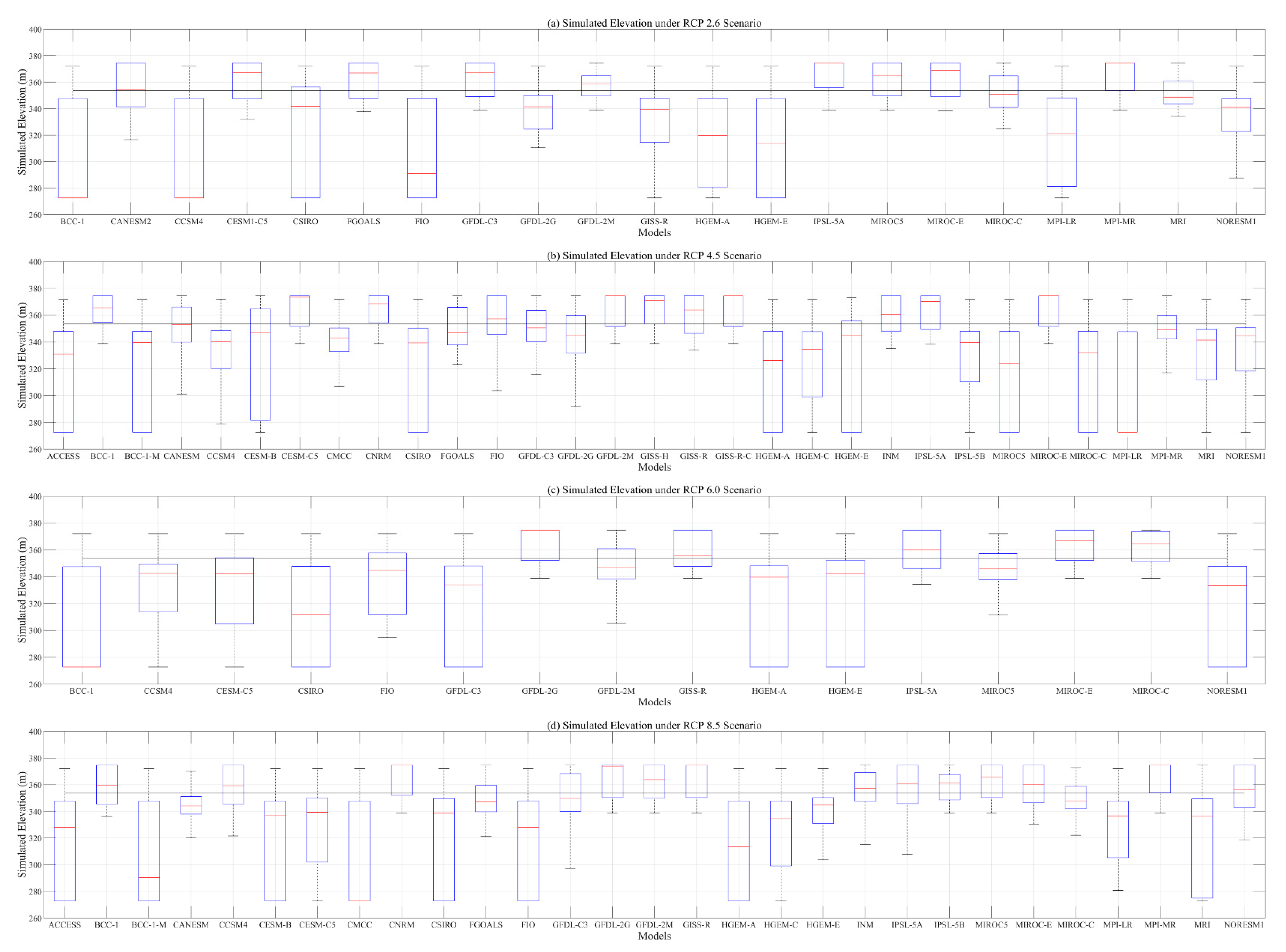
• The simulated future mean of Lake Mead elevation (2013-2049) can go up to 21.8% below the observed historical mean Lake Mead elevation (1989-2012). Out of the total 145 projections of climate models (from both CMIP3 and CMIP5), 44 projections predicted that the future mean elevation could go below 304.8 m (1000 ft), while 82 projections predicted that it could go below the historical mean elevation. The number of projections suggesting a drop in elevation in the future was only marginally higher than that of those suggesting otherwise. Hence, there is no definite consensus among these projections as to whether the lake level will drop in the future or not.
• Fifty-nine (27) out of the total 97 (48) climate and hydrological projections from the CMIP3 (CMIP5) model ensembles predicted the future mean Lake Mead level dropping below the historical mean level.
• Future mean lake level going below the historical mean is more likely for the emission scenario A1b (RCP 6.0) than the others in the CMIP3 (CMIP5) model ensembles.
• Mean reliabilities of water supply from Lake Mead to LVV for the future period were obtained to be the highest with the B1 emission scenario (lower carbon emission path) and to be the lowest with the A1b emission scenario (intermediate carbon emission path), among the CMIP3 model ensembles. With the CMIP5 model ensembles, mean reliabilities were found to be the highest with RCP 8.5 (highest GHG emission scenario) and to be the lowest with RCP 6.0 (intermediate GHG emission scenario).

Similar analyses can be conducted for other regions to obtain future water supply and demand scenarios under changing climate conditions with a growing population. Moreover, water management policies implemented in this study can be combined with more advanced and robust practices to curb demand in the future. This study may be helpful for water planners to prepare a water budget for the future and for water managers to evaluate multiple conservation practices through demand-side management.

References

1. Middelkoop, H.; Daamen, K.; Gellens, D.; Grabs, W.; Kwadijk, J.C.; Lang, H.; Parmet, B.W.; Schädler, B.; Schulla, J.; Wilke, K. Impact of climate change on hydrological regimes and water resources management in the Rhine basin. Clim. Chang. 2001, 49, 105–128. [Google Scholar] [CrossRef]
2. Tortajada, C.; Biswas, A.K. The rapidly changing global water management landscape. Int. J. Water Resour. Dev. 2017, 33, 849–852. [Google Scholar] [CrossRef]
3. Brekke, L.D.; Miller, N.L.; Bashford, K.E.; Quinn, N.W.; Dracup, J.A. Climate change impacts uncertainty for water resources in the San Joaquin River Basin, California1. J. Am. Water Resour. Assoc. 2004, 40, 149–164. [Google Scholar] [CrossRef]
4. Nyaupane, N.; Thakur, B.; Kalra, A.; Ahmad, S. Evaluating Future Flood Scenarios Using CMIP5 Climate Projections. Water 2018, 10, 1866. [Google Scholar] [CrossRef] [Green Version]
5. Thakur, B.; Kalra, A.; Miller, W.P.; Lamb, K.W.; Lakshmi, V.; Tootle, G. Linkage between ENSO Phases and western US Snow Water Equivalent. Atmos. Res. 2020, 236, 104827. [Google Scholar] [CrossRef]
6. Tamaddun, K.A.; Kalra, A.; Bernardez, M.; Ahmad, S. Effects of ENSO on Temperature, Precipitation, and Potential Evapotranspiration of North India’s Monsoon: An Analysis of Trend and Entropy. Water 2019, 11, 189. [Google Scholar] [CrossRef] [Green Version]
7. US Environmental Protection Agency (USEPA). Climate Change Indicators: U.S. and Global Temperature. 2015. Available online: https://www.epa.gov/climate-indicators/climate-change-indicators-us-and-global-temperature (accessed on 17 March 2017).
8. Ragab, R.; Prudhomme, C. Sw—soil and Water: Climate change and water resources management in arid and semi-arid regions: Prospective and challenges for the 21st century. Biosyst. Eng. 2002, 81, 3–34. [Google Scholar] [CrossRef]
9. Arnell, N.W. Climate change and global water resources: SRES emissions and socio-economic scenarios. Glob. Environ. Chang. 2004, 14, 31–52. [Google Scholar] [CrossRef]
10. Fu, G.; Charles, S.P.; Chiew, F.H. A two-parameter climate elasticity of streamflow index to assess climate change effects on annual streamflow. Water Resour. Res. 2007, 43. [Google Scholar] [CrossRef]
11. Xu, C.-Y.; Vandewiele, G. Parsimonious monthly rainfall-runoff models for humid basins with different input requirements. Adv. Water Resour. 1995, 18, 39–48. [Google Scholar] [CrossRef]
12. Brekke, L.D. Climate Change and Water Resources Management: A Federal Perspective; DIANE Publishing: Darby, PA, USA, 2009. [Google Scholar]
13. Thakur, B.; Kalra, A.; Ahmad, S.; Lamb, K.W.; Lakshmi, V. Bringing statistical learning machines together for hydro-climatological predictions-Case study for Sacramento San joaquin River Basin, California. J. Hydrol. Reg. Stud. 2020, 27, 100651. [Google Scholar] [CrossRef]
14. Tamaddun, K.A.; Kalra, A.; Ahmad, S. Spatiotemporal variation in the continental US streamflow in association with large-scale climate signals across multiple spectral bands. Water Res. Manag. 2019, 33, 1947–1968. [Google Scholar] [CrossRef]
15. Joshi, N.; Bista, A.; Pokhrel, I.; Kalra, A.; Ahmad, S. Rainfall-Runoff Simulation in Cache River Basin, Illinois, Using HEC-HMS. In Proceedings of the World Environmental and Water Resources Congress: Watershed Management, Irrigation and Drainage, and Water Resources Planning and Management, Pittsburgh, PA, USA, 19–23 May 2019. [Google Scholar]
16. SNWA. Water Resource Plan 2015; Southern Nevada Water Authority: Las Vegas, NV, USA, 2015.
17. Christensen, N.; Lettenmaier, D.P. A multimodel ensemble approach to assessment of climate change impacts on the hydrology and water resources of the Colorado River Basin. Hydrol. Earth Syst. Sci. 2006, 3, 3727–3770. [Google Scholar] [CrossRef] [Green Version]
18. Dawadi, S.; Ahmad, S. Changing climatic conditions in the Colorado River Basin: Implications for water resources management. J. Hydrol. 2012, 430, 127–141. [Google Scholar] [CrossRef]
19. Mehran, A.; AghaKouchak, A.; Nakhjiri, N.; Stewardson, M.J.; Peel, M.C.; Phillips, T.J.; Ravalico, J.K. Compounding impacts of human-induced water stress and climate change on water availability. Sci. Rep. Nat. 2017, 7, 1–9. [Google Scholar] [CrossRef] [PubMed] [Green Version]
20. Joshi, N.; Dongol, R. Severity of climate induced drought and its impact on migration: A study of Ramechhap District, Nepal. Trop. Agri. Res. 2018, 29, 194–211. [Google Scholar] [CrossRef] [Green Version]
21. Christensen, J.H.; Boberg, F.; Christensen, O.B.; Lucas-Picher, P. On the need for bias correction of regional climate change projections of temperature and precipitation. Geophy. Res. Lett. 2008, 35. [Google Scholar] [CrossRef]
22. Teutschbein, C.; Seibert, J. Regional climate models for hydrological impact studies at the catchment scale: A review of recent modeling strategies. Geogr. Compass 2010, 4, 834–860. [Google Scholar] [CrossRef] [Green Version]
23. Varis, O.; Kajander, T.; Lemmelä, R. Climate and water: From climate models to water resources management and vice versa. Clim. Chan. 2004, 66, 321–344. [Google Scholar] [CrossRef]
24. Casanueva, A.; Herrera, S.; Fernández, J.; Gutiérrez, J.M. Towards a fair comparison of statistical and dynamical downscaling in the framework of the EURO-CORDEX initiative. Clim. Chan. 2016, 137, 411–426. [Google Scholar] [CrossRef] [Green Version]
25. IPCC. Climate Change 2013: The Physical Science Basis; Cambridge University Press: Cambridge, UK, 2013. [Google Scholar]
26. Pierce, D.W.; Cayan, D.R.; Maurer, E.P.; Abatzoglou, J.T.; Hegewisch, K.C. Improved bias correction techniques for hydrological simulations of climate change. J. Hydrometeo. 2015, 16, 2421–2442. [Google Scholar] [CrossRef]
27. Gutiérrez, J.M.; Maraun, D.; Widmann, M.; Huth, R.; Hertig, E.; Benestad, R.; San Martín, D. An intercomparison of a large ensemble of statistical downscaling methods over Europe: Results from the VALUE perfect predictor cross-validation experiment. Int. J. Climatol. 2018, 39, 3750–3785. [Google Scholar] [CrossRef]
28. Cioffi, F.; Conticello, F.; Lall, U.; Marotta, L.; Telesca, V. Large scale climate and rainfall seasonality in a Mediterranean Area: Insights from a non-homogeneous Markov model applied to the Agro-Pontino plain. Hydrol. Proces. 2017, 31, 668–686. [Google Scholar] [CrossRef]
29. Fowler, H.J.; Blenkinsop, S.; Tebaldi, C. Linking climate change modelling to impacts studies: Recent advances in downscaling techniques for hydrological modelling. Int. J. Climatol. 2007, 27, 1547–1578. [Google Scholar] [CrossRef]
30. Tang, J.; Niu, X.; Wang, S.; Gao, H.; Wang, X.; Wu, J. Statistical downscaling and dynamical downscaling of regional climate in China: Present climate evaluations and future climate projections. J. Geophy. Res. 2016, 121, 2110–2129. [Google Scholar] [CrossRef] [Green Version]
31. Ayar, P.V.; Vrac, M.; Bastin, S.; Carreau, J.; Déqué, M.; Gallardo, C. Intercomparison of statistical and dynamical downscaling models under the EURO-and MED-CORDEX initiative framework: Present climate evaluations. Clim. Dyn. 2016, 46, 1301–1329. [Google Scholar] [CrossRef] [Green Version]
32. Ahmad, S.; Simonovic, S.P. System dynamics modeling of reservoir operations for flood management. J. Comput. Civil Eng. 2000, 14, 190–198. [Google Scholar] [CrossRef]
33. Shrestha, E.; Ahmad, S.; Johnson, W.; Batista, J.R. The carbon footprint of water management policy options. Energy Policy 2012, 42, 201–212. [Google Scholar] [CrossRef]
34. Sterman, J.D. Business Dynamics: Systems Thinking and Modeling for A Complex World; Irwin/McGraw-Hill: Boston, MA, USA, 2000. [Google Scholar]
35. Mirchi, A.; Madani, K.; Watkins, D.; Ahmad, S. Synthesis of system dynamics tools for holistic conceptualization of water resources problems. Water Resour. Manag. 2012, 26, 2421–2442. [Google Scholar] [CrossRef]
36. Winz, I.; Brierley, G.; Trowsdale, S. The use of system dynamics simulation in water resources management. Water Resour. Manag. 2009, 23, 1301–1323. [Google Scholar] [CrossRef]
37. Stave, K.A. A system dynamics model to facilitate public understanding of water management options in Las Vegas, Nevada. J. Environ. Manag. 2003, 67, 303–313. [Google Scholar] [CrossRef]
38. Qaiser, K.; Ahmad, S.; Johnson, W.; Batista, J. Evaluating the impact of water conservation on fate of outdoor water use: A study in an arid region. J. Environ. Manag. 2011, 92, 2061–2068. [Google Scholar] [CrossRef] [PubMed]
39. Ahmad, S.; Prashar, D. Evaluating municipal water conservation policies using a dynamic simulation model. Water Resour. Manag. 2010, 24, 3371–3395. [Google Scholar] [CrossRef]
40. Dawadi, S.; Ahmad, S. Evaluating the impact of demand-side management on water resources under changing climatic conditions and increasing population. J. Environ. Manag. 2013, 114, 261–275. [Google Scholar] [CrossRef]
41. Brekke, L.; Thrasher, B.; Maurer, E.; Pruitt, T. Downscaled CMIP3 and CMIP5 Hydrology Projections: Release of Hydrology Projections, Comparison With Preceding Information, and Summary of User Needs; US Department of the Interior-Bureau of Reclamation: Denver, CO, USA, 2014.
42. Ficklin, D.L.; Stewart, I.T.; Maurer, E.P. Climate change impacts on streamflow and subbasin-scale hydrology in the Upper Colorado River Basin. PLoS ONE 2013, 8, e71297. [Google Scholar] [CrossRef] [PubMed]
43. Sun, Q.; Miao, C.; Duan, Q. Comparative analysis of CMIP3 and CMIP5 global climate models for simulating the daily mean, maximum, and minimum temperatures and daily precipitation over China. J. Geophys. Res. Atmos. 2015, 120, 4806–4824. [Google Scholar] [CrossRef]
44. US Census Bureau (USCB). QuickFacts Clark County, Nevada. 2015. Available online: https://www.census.gov/quickfacts/clarkcountynevada (accessed on 18 January 2016).
45. Gorelow, A.S.; Skrbc, P. Climate of Las Vegas, Nevada; National Oceanic and Atmospheric Administration: Washington, DC, USA, 2005.
46. SNWA. Water Resources Plan 2009; Southern Nevada Water Authority: Las Vegas, NV, USA, 2009.
47. SNWA. Water Conservation Plan 2014–2018; Southern Nevada Water Authority: Las Vegas, NV, USA, 2014.
48. Ford, F.A. Modeling the Environment: An Introduction to System Dynamics Models of Environmental Systems; Island Press: Washington, DC, USA, 1999. [Google Scholar]
49. Forrester, J.W. System dynamics, systems thinking, and soft OR. Syst. Dyn. Rev. 1994, 10, 245–256. [Google Scholar] [CrossRef]
50. Christensen, N.S.; Wood, A.W.; Voisin, N.; Lettenmaier, D.P.; Palmer, R.N. The effects of climate change on the hydrology and water resources of the Colorado River basin. Clim. Chang. 2004, 62, 337–363. [Google Scholar] [CrossRef]
51. Nash, L.L.; Gleick, P.H. The Colorado River Basin and Climatic Change: The Sensitivity of Streamflow and Water Supply to Variations in Temperature and Precipitation; US Environmental Protection Agency, Office of Policy, Planning, and Evaluation: Oakland, CA, USA, 1993.
52. US Bureau of Reclamation (USBR). Colorado River Simulation System: System Overview. 1985. Available online: http://www.usbr.gov/lc/region/programs/strategies/FEIS/index.html (accessed on 3 August 2017).
53. US Bureau of Reclamation (USBR). Record of Decision, Colorado River Interim Guidelines for Lower Basin Shortages and the Coordinated Operation for Lake Powell and Lake Mead; US Department of Interior-Bureau of Reclamation: Sacramento, CA, USA, 2007.
54. Center for Business and Economic Research (CBER). Population Forecasts: Long-Term Projections for Clark County; University of Nevada: Las Vegas, NV, USA, 2015. [Google Scholar]
55. Colby, B.G.; Jacobs, K.L. Arizona Water Policy: Management Innovations in an Urbanizing, Arid Region; Routledge: Washington, DC, USA, 2007. [Google Scholar]
56. CSU. Integrated Water Resources Plan: Final Report. Colorado Springs Utilities. USA. 2017. Available online: https://www.csu.org/CSUDocuments/iwrpreportfinal.pdf (accessed on 8 February 2020).
57. Zongxue, X.; Jinno, K.; Kawamura, A.; Takesaki, S.; Ito, K. Performance risk analysis for Fukuoka water supply system. Water Res. Manag. 1998, 12, 13–30. [Google Scholar] [CrossRef]
58. US Bureau of Reclamation (USBR). Downscaled CMIP3 and CMIP5 Climate and Hydrology Projections. 2013. Available online: http://gdo-dcp.ucllnl.org (accessed on 15 December 2016).
59. US Bureau of Reclamation (USBR). Lake Mead at Hoover Dam, Elevation. 2016. Available online: http://www.usbr.gov/lc/region/g4000/hourly/mead-elv.html (accessed on 17 August 2017).
60. US Bureau of Reclamation (USBR). Monthly Summary Report. 2016. Available online: http://www.usbr.gov/uc/water/rsvrs/ops/monthly_summaries/index.html (accessed on 17 August 2017).
61. US Bureau of Reclamation (USBR). Upper Colorado River Basin Consumptive Uses and Losses Report; US Department of the Interior-Bureau of Reclamation: Denver, CO, USA, 2015.
62. US Bureau of Reclamation (USBR). Natural Flow and Salt Computation Methods. 2012. Available online: http://www.usbr.gov/lc/region/g4000/NaturalFlow/documentation.html (accessed on 20 July 2017).
63. Las Vegas Convention and Visitors Authority (LVCVA). Historical Las Vegas Visitor Statistics (1970–2016). 2016. Available online: http://www.lvcva.com/press/statistics-facts/index.jsp (accessed on 10 October 2017).
64. Sovocool, K.; Morgan, M. Xeriscape Conversion Study Final Report; Southern Nevada Water Authority: Las Vegas, NV, USA, 2005.
65. Clark County, Nevada (CCN). Area Wide Reuse Study Las Vegas Valley Study Area. 2000. Available online: http://www.accessclarkcounty.com/depts/daqem/epd/waterquality/Documents/AreaWideReuseStudy.pdf (accessed on 18 September 2017).
66. US Bureau of Reclamation (USBR). Streamflow Data for the Virgin River and Little Colorado River. 2016. Available online: https://waterdata.usgs.gov/usa/nwis/ (accessed on 13 December 2017).
67. Brekke, L.; Thrasher, B.; Maurer, E.; Pruitt, T. Downscaled CMIP3 and CMIP5 Climate Projections: Release of Downscaled CMIP5 Climate Projections, Comparison with Preceding Information, and Summary of User Needs; US Department of the Interior-Bureau of Reclamation: Denver, CO, USA, 2013.
68. US Bureau of Reclamation (USBR). Lower Colorado River Water Accounting Report; US Department of the Interior-Bureau of Reclamation: Denver, CO, USA, 2015.
69. Moriasi, D.N.; Arnold, J.G.; Van Liew, M.W.; Bingner, R.L.; Harmel, R.D.; Veith, T. Model evaluation guidelines for systematic quantification of accuracy in watershed simulations. Trans. ASABE 2007, 50, 885–900. [Google Scholar] [CrossRef]
70. Qaiser, K.; Ahmad, S.; Johnson, W.; Batista, J.R. Evaluating water conservation and reuse policies using a dynamic water balance model. Environ. Manag. 2013, 51, 449–458. [Google Scholar] [CrossRef] [PubMed]
71. Rahaman, M.M.; Thakur, B.; Kalra, A.; Ahmad, S. Modeling of GRACE-Derived Groundwater Information in the Colorado River Basin. Hydrology 2019, 6, 19. [Google Scholar] [CrossRef] [Green Version]
72. Rahaman, M.M.; Thakur, B.; Kalra, A.; Li, R.; Maheshwari, P. Estimating High-Resolution Groundwater Storage from GRACE: A Random Forest Approach. Environments 2019, 6, 63. [Google Scholar] [CrossRef] [Green Version]
73. Chen, J.; Brissette, F.P.; Leconte, R. Uncertainty of downscaling method in quantifying the impact of climate change on hydrology. J. Hydrol. 2011, 401, 190–202. [Google Scholar] [CrossRef]
74. Kendon, E.J.; Rowell, D.P.; Jones, R.G.; Buonomo, E. Robustness of future changes in local precipitation extremes. J. Clim. 2008, 21, 4280–4297. [Google Scholar] [CrossRef]
75. Lin, M.; Huybers, P. Revisiting whether recent surface temperature trends agree with the CMIP5 ensemble. J. Clim. 2016, 29, 8673–8687. [Google Scholar] [CrossRef] [Green Version]
76. Tebaldi, C.; Knutti, R. The use of the multi-model ensemble in probabilistic climate projections. Mathema. Phys. Eng. Sci. 2007, 365, 2053–2075. [Google Scholar] [CrossRef]
77. Pierce, D.W.; Barnett, T.P.; Santer, B.D.; Gleckler, P.J. Selecting global climate models for regional climate change studies. Natio. Acad. Sci. 2009, 106, 8441–8446. [Google Scholar] [CrossRef] [Green Version]
78. Weigel, A.P.; Liniger, M.A.; Appenzeller, C. Can multi-model combination really enhance the prediction skill of probabilistic ensemble forecasts? J. Atmos. Sci. 2008, 134, 241–260. [Google Scholar] [CrossRef]
79. Hagedorn, R.; Doblas-Reyes, F.J.; Palmer, T.N. The rationale behind the success of multi-model ensembles in seasonal forecasting—I. Basic concept. Tellus A. 2005, 57, 219–233. [Google Scholar] [CrossRef]
80. Gharbia, S.S.; Gill, L.; Johnston, P.; Pilla, F. Multi-GCM ensembles performance for climate projection on a GIS platform. Modeling Earth Syst. Environ. 2016, 2, 102. [Google Scholar] [CrossRef] [Green Version]
81. Yokohata, T.; Annan, J.D.; Collins, M.; Jackson, C.S.; Tobis, M.; Webb, M.J.; Hargreaves, J.C. Reliability of multi-model and structurally different single-model ensembles. Clim. Dyn. 2012, 39, 599–616. [Google Scholar] [CrossRef] [Green Version]
82. Najafi, M.R.; Moradkhani, H. Ensemble combination of seasonal streamflow forecasts. J. Hydrolo. Eng. 2016, 21, 04015043. [Google Scholar] [CrossRef]
83. Shi, H.; Li, T.; Liu, R.; Chen, J.; Li, J.; Zhang, A.; Wang, G. A service-oriented architecture for ensemble flood forecast from numerical weather prediction. J. Hydrol. 2015, 527, 933–942. [Google Scholar] [CrossRef] [Green Version]
84. McSweeney, C.F.; Jones, R.G.; Lee, R.W.; Rowell, D.P. Selecting CMIP5 GCMs for downscaling over multiple regions. Clim. Dyn. 2015, 44, 3237–3260. [Google Scholar] [CrossRef] [Green Version]
85. Ahammed, S.J.; Homsi, R.; Khan, N.; Shahid, S.; Shiru, M.S.; Mohsenipour, M.; Yuzir, A. Assessment of changing pattern of crop water stress in Bangladesh. Environ. Dev. Sustain. 2019, 1–19. [Google Scholar] [CrossRef]
86. Dai, A. Precipitation characteristics in eighteen coupled climate models. J. Clim. 2006, 19, 4605–4630. [Google Scholar] [CrossRef] [Green Version]
87. Hohenegger, C.; Brockhaus, P.; Schär, C. Towards climate simulations at cloud-resolving scales. Meteorol. Z. 2008, 17, 383–394. [Google Scholar] [CrossRef]
88. Stephens, G.L.; L’Ecuyer, T.; Forbes, R.; Gettelmen, A.; Golaz, J.C.; Bodas-Salcedo, A.; Haynes, J. Dreary state of precipitation in global models. J. Geophys. Res. 2010, 115, D24211. [Google Scholar] [CrossRef]
89. Rasmussen, R.; Ikeda, K.; Liu, C.; Gochis, D.; Clark, M.; Dai, A.; Yates, D. Climate change impacts on the water balance of the Colorado headwaters: High-resolution regional climate model simulations. J. Hydrometeor. 2014, 15, 1091–1116. [Google Scholar] [CrossRef]
90. Pan, L.L.; Chen, S.H.; Cayan, D.; Lin, M.Y.; Hart, Q.; Zhang, M.H.; Wang, J. Influences of climate change on California and Nevada regions revealed by a high-resolution dynamical downscaling study. Clim. Dyn. 2011, 37, 2005–2020. [Google Scholar] [CrossRef] [Green Version]
91. Kendon, E.J.; Ban, N.; Roberts, N.M.; Fowler, H.J.; Roberts, M.J.; Chan, S.C.; Wilkinson, J.M. Do convection-permitting regional climate models improve projections of future precipitation change? Bull. Am. Meteorol. Soc. 2017, 98, 79–93. [Google Scholar] [CrossRef]
92. Warner, T.T. Numerical Weather and Climate Prediction; Cambridge University Press: Cambridge, UK, 2010. [Google Scholar]
93. Chaturvedi, R.K.; Joshi, J.; Jayaraman, M.; Bala, G.; Ravindranath, N.H. Multi-model climate change projections for India under representative concentration pathways. Curr. Sci. 2012, 103, 791–802. [Google Scholar]
94. Hoerling, M.; Lettenmaier, D.; Cayan, D.; Udall, B. Reconciling projections of Colorado River streamflow. Southwest Hydrol. 2009, 8, 20–21. [Google Scholar]
Figure 1. Location map of the study area—the Las Vegas Valley.
Hydrology 07 00016 g001
Figure 2. A simplified conceptual diagram of the system dynamics model.
Hydrology 07 00016 g002
Figure 3. (a) Comparison between the observed and simulated water demand for Las Vegas Valley (LVV) from 1989 to 2012. (b) Plot showing linear relationship between observed and simulated water demand in the LVV from 1989 to 2012. (c) Comparison between the observed and simulated Lake Mead levels for the historical period from 1989 to 2012. (d) Plot showing correlation between the observed and simulated Lake Mead level for the historical period from 1989 to 2012. (e) Plot showing the historical and simulated future water demand in monthly time series.
Hydrology 07 00016 g003
Figure 4. Boxplots of future simulated elevations of Lake Mead from 2013 to 2049 for the various CMIP3 climate models under emission scenarios (a) A1b, (b) A2, and (c) B1. The solid lines represent the historical mean elevation of Lake Mead.
Hydrology 07 00016 g004
Figure 5. Boxplots of future simulated elevations of Lake Mead from 2013 to 2049 for the various CMIP5 climate models under emission scenarios (a) RCP 2.6, (b) RCP 4.5, (c) RCP 6.0, and (d) RCP 8.5. The solid lines represent the historical mean elevation of Lake Mead.
Hydrology 07 00016 g005