Article

Assessment of Erosion in River Basins: A Distributed Model to Estimate the Sediment Production over Watersheds by a 3-Dimensional LS Factor in RUSLE Model

1
Department of Biotechnology and Territory, University of Molise, 86100 Campobasso, Italy
2
Department of Civil, Architectural and Environmental Engineering, Federico II University, 80134 Naples, Italy
*
Author to whom correspondence should be addressed.
Hydrology 2020, 7(1), 13; https://doi.org/10.3390/hydrology7010013
Submission received: 19 December 2019 / Revised: 18 February 2020 / Accepted: 19 February 2020 / Published: 24 February 2020

Abstract

:
Erosive processes influence on several phenomena. In particular, they could influence on land depletion, on vegetation weakening, on aggradation phenomena of intermediate, and plain reaches of rivers, on waterways interruption due to overaggradation phenomena caused by floods, and on the losses of water volumes that may be stored in reservoirs. Among the models proposed in the literature for the prediction of erosion on the annual scale, one of the most widely used is the Revised Universal Soil Loss Equation (RUSLE). In the present paper, starting from the definition of the original model, the authors improved the important combined slope length and slope angle (LS-factor), taking into account the mutual interaction of solid particles, in terms of path and confluences, so as to transform the model, which was first classified on a slope scale or at most on a parcel one, into a distributed model on a basin scale. The use of a distributed approach is an integral part of the analysis of the hydrogeological risk. In this way, it is possible to obtain a map of the erodibility of any basin, from which to derive the most vulnerable areas. The proposed methodology has been tested on the Camastra Basin, located in Basilicata Region of Southern Italy.

1. Introduction

Soil erosion in river basins and the resulting sediment supply to the river network are two phenomena that are strongly interconnected and require great attention due to the problems associated with them. In fact, the occurrence of an erosive process can often entail a troubling degradation of the environment: firstly, the characteristics of the hillsides get lost due to the material removal, and secondly there may be a significant reduction in the capacity of the volume of a reservoir, if present in the basin, with a consequent decrease in the volumes of water that can be delivered to users [1,2,3,4].
Erosive processes, in the widest meaning of the phenomenon, are a combination of disaggregation, mobilization, and removal of sediments from the solid matrix of the soil, leading to a more or less intense alteration of the surface level. The most damaging characteristic of the erosive phenomenon is the speed of its occurrence, so it is usual to distinguish two types of erosion: normal or geological erosion occurs when the speed of degradation is sufficiently slow, while there is an accelerated erosion when the solid material removal happens faster than its deposition [5]. In the first case the system is in equilibrium, and therefore the thickness is unaltered, because the speed at which the soil is formed by the decomposition of the rocks compensates for the loss suffered; in the second case, on the contrary, the final result is often the surface outcrop of the below bare rock. In particular, there is either a thinning of the arable layer, with reference to agricultural soils, as well as a reduction of the surface horizons in the case of natural soils. The direct consequences are a reduction of the useful thickness for the roots’ plants, of the nutrient reserve, and of the water retention capacity. The main agents of this alteration are water, glaciers, and wind. At the Italian latitudes, the damages are mainly caused by water erosion while, on the contrary, wind erosion can be considered of minor importance, although in coastal sandy areas it can be found with a certain frequency [6]. In addition to water erosion, there can also be a cross-sectional erosion of the riverbed, which can be both vertical and lateral, and gravitational instabilities on the slopes, such as surface and deep landslides [7]. The phenomena of hydrogeological and hydraulic instability in Italy represent a long-standing problem, since the geological and geomorphological characteristics of the land entail a very high exposure to the risk of landslides and floods. Several studies [8,9,10,11], among the others, have shown that the Italian peninsula has the highest number of hydrogeological instabilities in Europe, which have often caused damage to people, structures, and infrastructures, with a significant economic and social impact. Consequently, knowing these phenomena is essential for estimating the level of hydrogeological risk, caused both by the sediment supply deriving from flooding and deforestation phenomena, as well as by the construction of dams and crossbars on branches of the hydrographic network.
The development of soil erosion prediction techniques was born with Cook’s studies, in 1937, in order to identify the main variables that affected the transformations of the territory due to the action of water [12]. A few years later, Zingg published the first equation that mathematically described soil loss as a function of topography alone [13]. Just one year later, Smith added factors to the equations that represented the influence of plant cover and anthropogenic practices [14]. Several authors prepared graphs and tables by collecting numerous experimental data, obtained for different conditions of land use: in the United States, the forecasts obtained from these equations were decisive for land management and the adoption of conservative practices to limit the damage caused by water erosion, so much so that the need to derive a nationally valid equation was established [15]. Since the publication of those first studies, over the last 50 years a huge number of models have been developed to describe quantitatively the erosive phenomena, each operating at different spatial and temporal scales and especially with different levels of complexity in terms of input required. Moreover, it is also possible to use such models by means of web and desktop applications that automatically provide the results.
The choice among erosion models is very wide [16]. Therefore, it is necessary to pay attention to all the variables involved, the inputs and outputs and especially the spatial and temporal scales to be referred to. Sometimes, the choice is not immediate even after defining the requirements, since in most cases, models are not supported by explicit statements regarding the purposes and conditions for which they were designed, their limitations or indicators of the accuracy of their production [17]. Generally, the “best model” for describing processes does not exist, but it is widely known that a “good” model must satisfy the requirements of simplicity of implementation, reliability, completeness; moreover, it should be quite easy to use. The literature is full of correlations that, according to the characteristic parameters, allow the evaluation of a potential solid production [18]. Yet, the robustness of these correlations, based on regression analysis with very high margins of uncertainty, remains essentially limited to the sample used for the assessment. Moreover, if the level of conceptualization that allowed the representation of the process has a spatial scale (e.g., the whole basin) different from the one of the sample (e.g., a single parcel), the results often become unsatisfactory [19]. This overview provides an opportunity to identify the complexities and opportunities associated with erosion and risk mapping at basin scale: in order to obtain a more accurate evaluation, it is therefore necessary to reconsider the process, with accurate hypotheses and in a more appropriate way. However, Chaplot by using the Soil and Water Assessment Tool (SWAT) showed that sediment load is little affected by resolution of land-use map [20,21].
In this paper, the well-known Universal Soil Loss Equation (USLE) model [22] was chosen because its codification has found numerous positive results in reference to its vast experimentation, being constituted by an equation which appears to be very simple, but which completely encloses the physical meaning of the whole process. The popularity of this application is due, on one hand, to the technical robustness of the method and, on the other hand, to the lack of alternative models for the planning of conservation practices to control soil water erosion. The individual factors of the USLE have been often modified and improved, leading to a “new” model known as Revised Universal Soil Loss Equation (RUSLE) or Modified Universal Soil Loss Equation (MUSLE) [23,24,25,26,27], to apply the model to hillsides or wide basins, also thanks to the increase in the computational capacity of electronic computers, but especially with the spread of Geographic Information Systems (GIS), which have become an essential tool to obtain an accurate estimation of soil loss [28,29,30,31,32,33].
The principal aim of this study was the revisitation of the factors of the RUSLE model. In particular, the improvements focused on the slope Length and Slope angle (LS-Factor), initially the most critical parameter to be identified, but also the most important parameter in the estimation of soil loss due to erosion.
Finally, the other goal of the paper was coupling GIS with the erosion models to obtain an erodibility map, in order to identify the areas that need of mitigation interventions for the hydraulic protection of the territory, and to estimate the silting of reservoirs for a good management of them [34,35,36,37]. For this reason, the Camastra Basin was chosen to test the approach developed in this work because there is an important reservoir known as Camastra Reservoir.

2. Materials and Methods

2.1. The Study Area

The study case of this paper is the basin of the Camastra river, which belongs to the largest basin of the Basento River. The place is in Basilicata Region of the Southern Italy. This choice was dictated both by the environmental vulnerability of the region and by the presence of lots of data usable for the validation of the procedure proposed in this work. Its territory is mainly mountainous (46%) and hilly (46%) with a modest percentage of flat land (8%). The area of interest consists of about 10% limestone, dolomitic limestone, silica, and arenaceous stratified rocks. In the rest of the area there are soils with variable lithologies, from successions of clayey soils with limestone and arenaceous stone to deposits of loose clayey, sandy, and conglomerate rocks. The territory is mainly characterized by broadleaf woods and in general by an intense wood cover, with some sowing areas and hilly grasslands. The climate of the region can be defined as continental, with Mediterranean characteristics only in coastal areas. In fact, in the inland areas, especially in winter, the mildness is replaced by a harsh and humid climate. The main disturbances come from the Tyrrhenian side, and, due to the presence of the reliefs, they discharge the most consistent rains on the western part of the region, where, the average annual rainfall reaches values around 2000 mm (CFD Basilicata Region). It occupies the basins of the main Apennine rivers that flow into the Gulf of Taranto (Puglia Region): the Basento River, the Bradano River, the Cavone River, the Agri River, and the Sinni River. All these rivers having irregular hydraulic regime.
The Camastra River is the main tributary of the Basento river, which originates in the Northern Lucanian Apennines from the North-Western slopes of Monte Arioso, flows from the North-West to the South-East in the provinces of Potenza and Matera and ends into the Gulf of Taranto. The Camastra River falls entirely in Basilicata Region for about 1537 km and its basin occupies about 23% of the total area. In particular, it concerns Basilicata municipalities of Abriola, Calvello, Pignola, Marsicovetere, Viggiano, Marsico Nuovo, Sasso di Castalda, Laurenzana, and Anzi. Finally, before the confluence between Basento River and Camastra River, a dam locked the latter to make the artificial Camastra reservoir (see Figure 1).
In particular, the study area is located between the following coordinates (see Table 1).

2.2. The RUSLE Approach

As with any model, the use of the USLE model is limited to certain purposes but can always be optimized and improved. The result of one of these improvements is the RUSLE (Revised USLE) currently adopted by the United States Department of Agriculture (USDA) and by the Soil Conservation Service (SCS) as an official tool for predicting water erosion and planning soil conservation interventions in the USA [15].
In this paper, the geospatial distribution of the soil loss has been achieved by using a GIS-based method, result of the revisitation of each parameter of the USLE. The original model and most of its modifications come with the following expression:
A = R × K × LS × C × P
where: A is the average yearly soil loss of a parcel [ton/(year∙ha)]; R is the rainfall erosivity factor [MJ∙mm/(ha∙hr∙year)]; K is the soil erodibility factor [(ton∙ha∙h)/(MJ∙mm∙ha)]; LS is the topographic factor [dimensionless]; C is the cropping management factor [dimensionless]; P is the support practice factor [dimensionless].
The most substantial revision of the RUSLE considered by authors concerns the topographic factor LS. In fact, in the original version of the RUSLE [28], the spatial scale was a parcel one and the LS factor was characterized by the one-dimensional length of the parcel itself. The algorithm developed in this paper considers the total drained area upstream of a specific parcel, instead of its distance from the point of formation of the outflow, and it is based on the resolution of a continuity equation of the flow rates transiting the single parcels, so that the drainage path can be obtained from the Digital Terrain Model (DTM) of the area and the values of specific contribution for each parcel. In this way, thanks also to the introduction of GIS, it was possible to expand the spatial scale at basin level and to consider, for each parcel, the confluences of water and solid flows with a multidimensional method (see Section 2.2.5). All factors in Equation (1) were computed in a GIS environment. In particular, the software QGIS™ was chosen since it is more versatile in the customization of the model and it is simpler and more intuitive in the Graphical User Interface than other software, because it has been primarily developed in C++ and Python language.
Then, the total mass of eroded soil within a basin, estimated with the RUSLE represents the amount of gross erosion. It does not correspond to the solid material that actually deposits inside the reservoir that underlies the basin, which is defined as net erosion and represents a small percentage of the first [38]. This quantity can be evaluated in several ways [39,40], among which the most immediate are the difference between two bathymetric measurements carried out in different years [35] or the measurement of the solid flow transited during the same period through the closing section of the basin. In the literature, net erosion, evaluated from the sedimented volume in the reservoirs, is usually identified with the term Sediment Yield, Y.
The ratio between the quantity of sediments delivered to the reservoir through solid transport in the hydrographic network and that of eroded material, or rather the ratio between net erosion Y and gross erosion A, is defined as the solid yield coefficient or, more commonly, Sediment Delivery Ratio (SDR).
SDR = (net_erosion)/(gross_erosion) = Y/A
Lastly, using the obtained soil loss map as a hazard one, along with land use and population data to represent the damage, a global representation of the risk was also achieved (see flowchart in the following Figure 2).

2.2.1. R-Factor

Among the various climatic factors of an area, rain is the one that has the greatest impact on erosion. The rainfall erosivity factor, known as R, is a multi-year average index that measures the kinetic energy and intensity of precipitation to describe the effect of precipitation on rill and inter-rill erosion [41]. Kinetic energy is, indeed, an important factor in soil erosion by water, which is directly related to the climatic parameters of precipitations: it can lead to a greater or lesser degree of detachment and transport of solid particles downstream, in relation to the rainfall intensity.

2.2.2. K-Factor

The K-factor is a measure of the inner erodibility of a given soil with reference to the standard condition of a clean tilled continuous fallow parcel, so it has a unit of measurement equal to a mass per area per unit of rainfall erosivity R. Its values typically range from about 0.10 for soils with high clay content, to 0.45 for soils with prevalent sand content. The inner erodibility of soils depends on the interaction between biological and physical processes of stabilization and destabilization that occur within them. In particular, soil stabilization involves an increase of the critical threshold above which erosion occurs, while destabilization consists of an increase in the rate of erosion, e.g., a decrease of this critical threshold. Of course, the occurrence of these processes and their intensity are a function of the geolithological and hydrogeological characteristics of the area. For instance, soils altered by limestone or those on igneous rocks are the most resistant, unlike those on sediments such as sandstone, clay, or gypsum, but also the stratification of the different textures plays a key role.
For these reasons, the K-factor is obtained indirectly, either from the composition of the soil or from its grain size that require the knowledge of a large amount of data. Some of them are determined by laboratory tests, such as the percentages of organic material and those of clay, silt and sand, while others, such as the structure and permeability, derive from qualitative judgments. In addition, if affected by a strong spatial variability even within the same class of land use, its values could be distorted [42]: in these cases, a constant value throughout the study area should be gained, especially if the K-Factor assumes a lower weight in the estimation of soil loss than the other factors.

2.2.3. C-Factor

Vegetation and land use are the main factors controlling the intensity and frequency of surface runoff and consequently the resulting diffuse erosion.
Some studies have tried to evaluate C-Factor using vegetation factors derived from remote sensing, often combined, such as vegetation cover classification maps, spectral band relationships or vegetation spectral indices. There is a wide range of such parameters, but the Normalized Difference Vegetation Index (NDVI) is certainly the most widespread. The NDVI is defined by Rouse [43] as the ratio between the difference and the sum, respectively, between the Near Infra-Red spectral reflectance (NIR) and the Red one (R). In symbols:
NDVI = (NIR − R)/(NIR + R)
The evaluation of this index allows a direct estimation of the C-Factor, through relationships of different nature validated in different field tests. One example is the exponential relationship:
C = exp(−α (NDVI/(β − NDVI)))
where the α and β coefficients are often set at 2 and 1, respectively, because in several regions a linear correlation, for NDVI between 0.0 and 0.5, is the one that best approximates the real data, especially with reference to the climatic conditions typical of Europe [44].

2.2.4. P-Factor

Management practices generally influence erosion either by redirecting the flow along watercourses or by slowing it down. In the first case, the hydrographic network is modified, while in the second case the slope or direction of flow is altered with extended hydraulic systems, such as terraces or pointing systems such as check-dams. In most publications, the P factor is set at 1, regardless of land use and land size, due to the lack of information on the interventions carried out in the different areas of the basins.

2.2.5. LS-Factor

In the original versions of the USLE [22] and the RUSLE [15], the spatial scale was parcel based and the LS-Factor was characterized by the one-dimensional length of the parcel.
The inconsistencies that have appeared in the application of the method up to that moment have always been attributed to the impossibility of the LS-Factor, so computed, to take full account of all transport mechanisms, especially when the geometry of the hillsides becomes complex. The method, in fact, did not explicitly contemplate the convergence or divergence of river basins. For basins of the same area, a convergent basin should have more sediments than a divergent basin, because this is exactly the behavior that is observed in nature.
To this aim, various algorithms have been proposed in the literature. A basic distinction can be made between one-dimensional flow algorithms, which transfer all matter from the source cell to a single downstream cell, and multidimensional flow algorithms, which divide the flow of matter from one cell to multiple receiving cells. Yet, this distinction is not purely technical. In fact, the former only allow a parallel and convergent flow, while the latter also consider divergent flows.
Nowadays, GIS technology allows a relatively simple construction and management of digital elevation models which, in principle, allow the calculation of the area of the contributing unit, so that the complex nature of the topography can be considered.
The catchment area can be divided into several contributing cells (pixels), each of which is associated with the central cell of a sub-matrix [3 × 3]. The erosion attributed to this cell results in the solid contribution in the downstream adjacent cells, while the contribution received from each cell becomes proportional to the product between two averages weighed on geometric factors, which depend on the direction of the flow. If the values of the inlet contributing area A, the length of the boundary crossed by the flow x, and the size of the plot side D, are known, the L-subfactor of a single pixel (i, j) can be calculated as follows [38]:
L i , j = ( A i , j i n + D 2 ) m + 1 A i , j i n m + 1 D m + 2 x i , j m ( 22.13 ) m
The exponent m is correlated to the ratio β between the rill erosion, caused by surface runoff, and the impact erosion, through the equation [45]:
m = β/(1 + β)
The expression achieved for β was experimentally obtained from the analysis of a soil moderately susceptible to both kinds of erosion:
β = (sinθ/0.0896)/(3∙(sinθ)0.8 + 0.56)
where θ is the slope steepness.
Moreover, the length of the boundary that can be crossed by the incoming flow (Di,j) in each pixel (D × D) is identified in the X,Y plane by azimuth angles (αi,j):
Di,j = D∙xi,j = D∙(sinαi,j + cosαi,j)
In topography, the determination of angles is carried out with the triangulation method, in which each triangle considered has always acute angles and each angle is measured by using a theodolite and a mobile reference system. Considering, therefore, for triangular parcels, the outflow starting from a vertex, the outflow direction, coinciding with that of maximum slope, that is the direction of the minimum path, corresponds to the height of the triangle with respect to the opposite side to that vertex. The azimuth angle of a generic parcel is measured with respect to the outflow direction of the previous parcel, and corresponds, generically, to the angle between the heights of two adjacent triangles, starting from the common vertex. It can be demonstrated, through geometric reasoning, that this angle is always less than 3π/4, so the sum of sine and cosine of this angle always assumes positive values.
In a GIS environment, the determination of azimuth angles is completely different, especially since a stationary reference system is used, so that angles can assume any value belonging to the interval [0; 2π] and, in particular, in the interval [3π/4; 7π/4], the sum of sine and cosine of the azimuth angle is negative. As a consequence, the length Di,j is underestimated or even negative, so it is necessary to modify appropriately the Equation (8), taking sine and cosine in modulus:
Di,j = D∙xi,j = D∙(|sinαi,j|+|cosαi,j|)
While, with regard to the S-subfactor, two conditions were identified:
  • for hillsides longer than 4.6 m (15 feet), it is evaluated with a piecewise function:
    S i , j = { 10.8 sin θ i , j + 0.3 s i , j < 9 % 16.8 sin θ i , j 0.5 s i , j 9 %
  • for hillsides of less than 4.6 m in length, the following relationship must be used:
    S i , j = 3 ( sin θ i , j ) 0.8 + 0.56
The Equations (10) and (11) originally referred to a hillside scale, but as they were calibrated, they can be attributed to a single pixel (i, j).

3. Results and Discussion

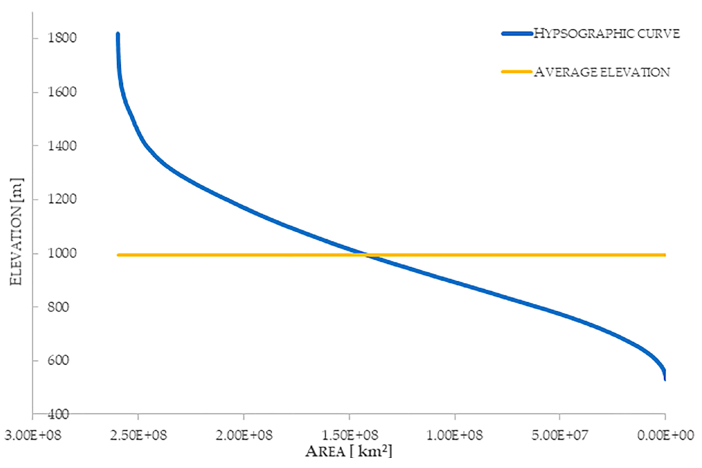
The basin, generated through QGIS™, is characterized by a watershed line of about 97 km and by an extension of about 350 km2. To carry out a first morphometric analysis of the study case, the Drainage Density (DD) and the hypsographic curve of the basin were calculated using some basic statistics for the numeric fields of the layers through the ‘r.report’© GRASS™ tool. The DD value is 1.02 km/km2, while the hypsographic curve is shown in the Figure 3 below.
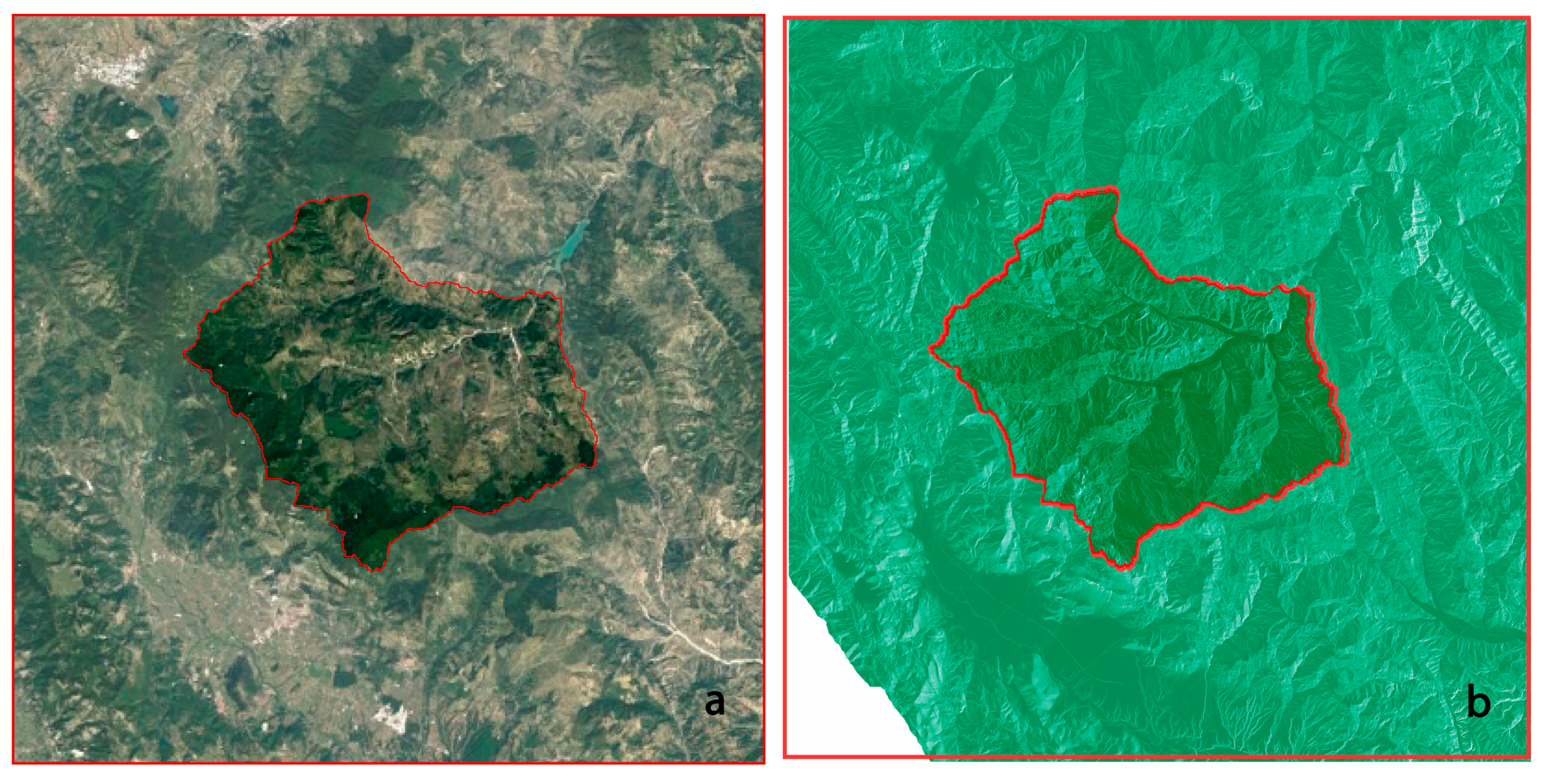
In order to validate the obtained results, the relief on the Google™ Earth Pro platform (Figure 4a) has been compared with the one produced by the QGIS™ software (Figure 4b).

3.1. Model Setting and Input Parameters

The first technical aspect of this procedure concerns the use of GIS even before the actual hydrological analysis, since GIS were also involved in the identification of the basin itself. In particular, given the smaller size of the case study compared to the regional one, the first step was the summary identification of the watershed’s location with the aggregation of the concerning municipal geometries.
The second step consisted in the obtaining raster map of flow accumulation and drainage direction, as well as the location of the catchment’s streams and sub-basins by using the hydrological tools of the GRASS™ GIS plugin, ‘r.watershed’©. The input data required by the tool is the raster DEM, chosen with the highest resolution available (5 m). Instead, the coordinates of the water outlet, picked at the inlet to the Camastra Reservoir, along with the drainage direction map previously obtained, were the input data requested by the GRASS tool ‘r.water.outlet’© to generate the watershed basin.
Then, each parameter of RUSLE was evaluated considering both the GIS applicability and the extent and reliability of the available data. In fact, the resulting model is as consistent as possible with the average accuracy of the input parameters, so that they had equal weight in the final matrix. In addition, the relationships were chosen so as to be independent of the case study. Then, by combining the results, it was possible to derive the spatialization of the average annual soil loss over the entire basin.

3.1.1. R-Factor

In order to choose the formula to be used for the evaluation of the erosivity factor, it was necessary to identify the locations of the pluviographic stations for measuring the rainfall depths and then to analyze the available data. In Camastra Basin, used to test the approach presented in this work, three stations have been identified and, for each of them, a preliminary analysis of the available historical series has been carried out.
It has been found that, despite being in use until now, most hydrological annals report a scarce number of pluviographic data (see Table 2).
It was therefore not possible to use the rigorous method proposed by Renard [15], but the total monthly rainfall heights recorded were obtained from the daily data and used to apply the equation proposed by Ferro [46], who extended the Modified Fournier Index (MFI) and, consequently the computation of the R-factor to N years of observation:
R = (4.17FF) − 152
where:
F F = 1 N j N 1 12 p i , j 2 p j
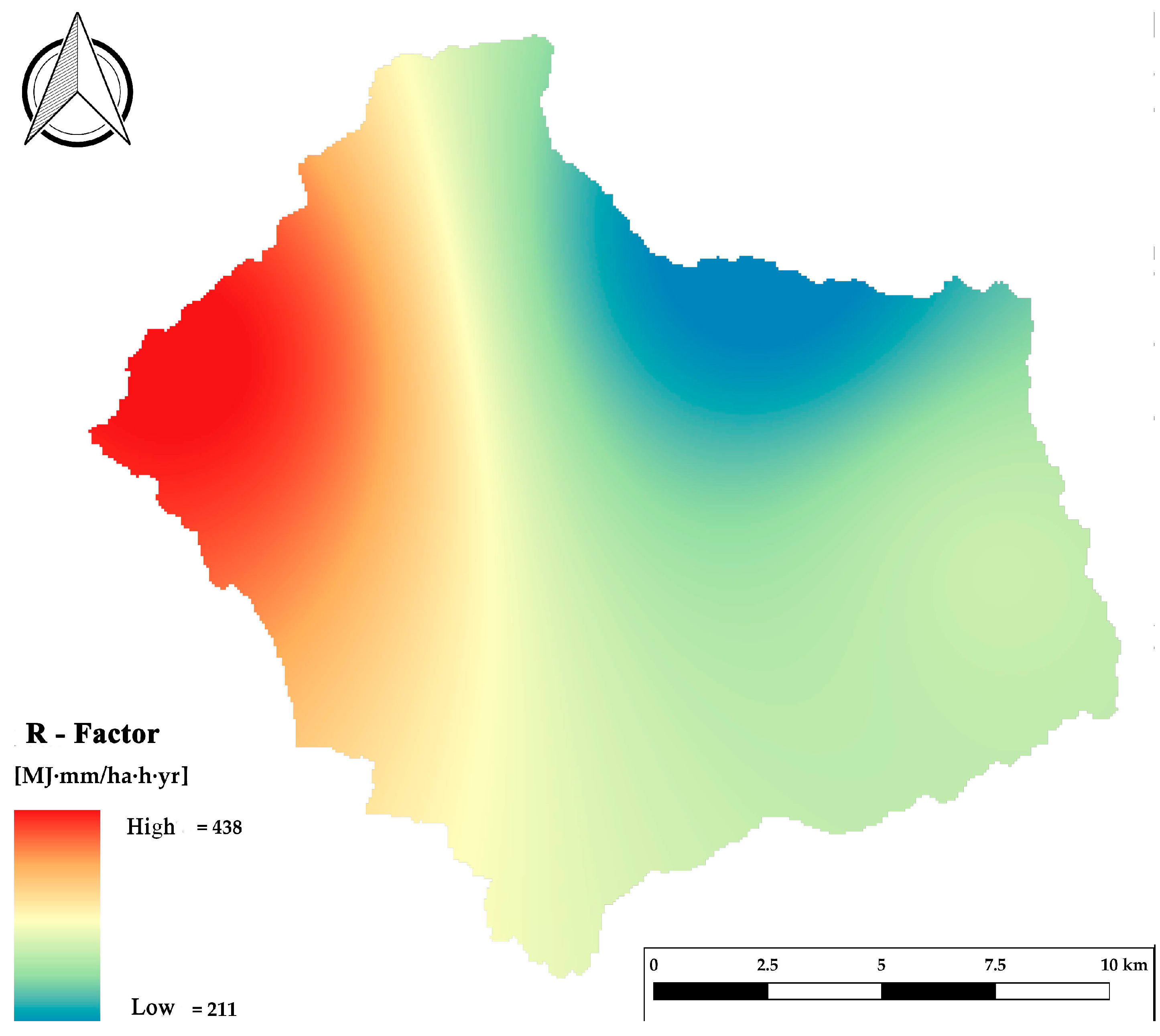
The R-values of each pluviographic station has been spatialized with a numerical approximation because, in comparison with other methods, allows a representation of more complex surfaces (see Figure 5). The linear interpolation was computed through the GRASS plugin ‘v.surf.idw’© which provides a DEM–based 3D interpolation from the vector point data containing the stations by Inverse Distance Squared Weighting method.

3.1.2. K-Factor

For the case study considered in the present work, K-Factor was seen to have less weight in estimating soil loss than the other factors and is characterized by a low standard deviation, so it was decided to use a constant value for the entire basin, 0.14, validated by several studies in situ [45,47].

3.1.3. C-Factor

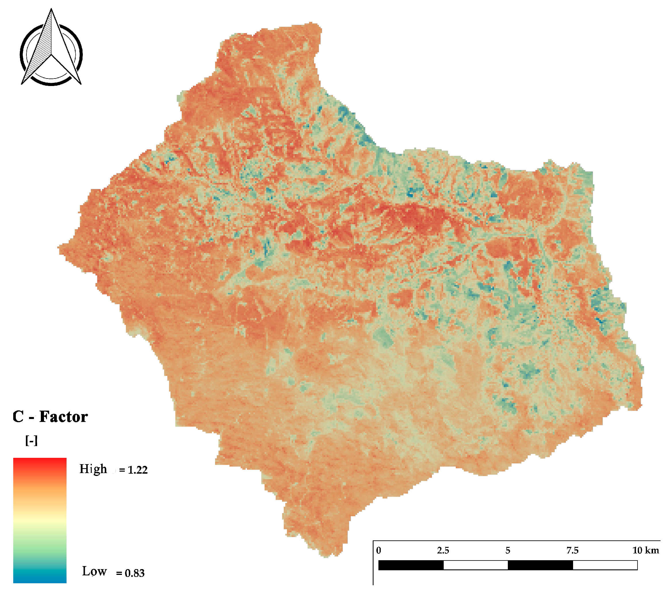
For the estimation of the coverage factor of the Camastra Basin, the satellite images, provided by the Landsat 8 satellite of NASA (2017), were acquired online and imported into QGIS™, after orthorectification according to the project’s reference system. To consider the most severe condition and, at the same time, minimize the effect of cloud cover and haze, images of December were chosen for each year of observation. The seasonal variability of vegetation greatly influences the assessment in areas characterized by a Mediterranean climate, especially because this seasonality is also found for rainfall events. The values of NDVI and, consequently, of the C-Factor have been obtained from these inputs with the QGIS™ ‘raster calculator’©, after having cut out the input layers using the extension of the basin as a mask (see Figure 6). In particular, satellite images related to red band and infrared band or rather, with reference to the remote system, related to reflectance bands B3 and B4 were used.

3.1.4. P-Factor

In the case of Camastra Basin, there are some anti-erosion practices, or rather extensive interventions such as planting, throughout the watershed of the Camastra, but they represent only a small part of the total catchment area. Farmers do not use erosion control practices. Land use has shown that agriculture is mostly cereal-based and satellite orthophotos [48] have shown that ploughing is rarely parallel to the contour lines. In this context, differentiating the P factor was considered inappropriate, so a unit value was therefore assigned for the entire extension of the basin [45]. This approach is also widely used in literature [31].

3.1.5. LS-Factor

QGIS™ provides two maps representing the L (Length) and S (Slope) factors via its GRASS™ extension. However, it uses equations only validated on the United States typical soils and, above all, those functions depend on the length of the slope and not on the contributing area: it was therefore preferred to manually implement the equations, starting from the DTM dataset (see Appendix A), with a resolution of 5 m, which was the most appropriate, as well as coinciding with the resolution used for other data, such as LULC (Land Use Land Cover) data [49] and NDVI data [48].
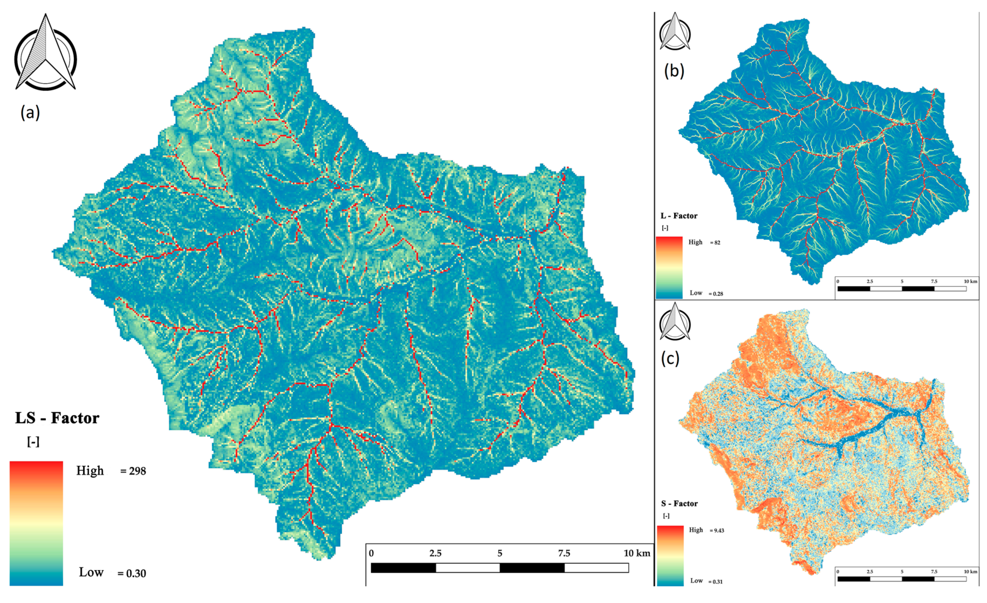
Then, in order to obtain the spatialization of the topographic factor, LS (see Figure 7a), L-Factor and S-Factor were calculated separately, as described in detail in the following paragraphs (see the following: “L-Subfactor” and “S-Subfactor” parts), and then multiplied together.

L-Subfactor

Given the amount of input data required by the Equation (8), the spatialization of the L-Factor involved several computations. The contributing area for each pixel (Ai,j-in), is the output ‘accumulation’ of the GRASS module ‘r.watershed’©. In particular, it offers for the calculation of the surface area both a one-dimensional method (SFD—Single Flow Direction) and a multidimensional method (MFD—Multiple Flow Direction). The latter was used because it distributes the water flow on all adjacent pixels with a lower elevation, using as weight factor for proportionality the slope of the same, so it was the most accurate for the purpose of this study.
Moreover, the measurements of the azimuth angles of the pixels of the basin were taken from the ‘drainage direction’ output of the already used GRASS ‘r.watershed’© module. These angles are the aspect values that indicate the direction in which the outflows are directed, measured counterclockwise from the East with centesimal degrees. The value 0 (zero) indicates that the pixel is a depressed area, while any negative values indicate that the surface flow is leaving the boundaries of the current geographical area. Multiplying the values by 45 gives the direction in degrees (see Section 2.2.5 and Figure 7b).

S-Subfactor

First of all, it needs to highlight that the resolution of DTM is equal to 5 m. Then, as far as the processing of the S-Subfactor, the slope function of McCool was always considered for hillsides longer than 4.6 m (see Section 2.2.5). In fact, in this work only the implementation of the function at times described by (11) for each pixel was done. The breaking point of the function is determined by the slope limit expressed as a percentage, which in itself is a function of the zenithal angles extracted from the DTM (see Figure 7c).

3.1.6. Estimate of Soil Loss

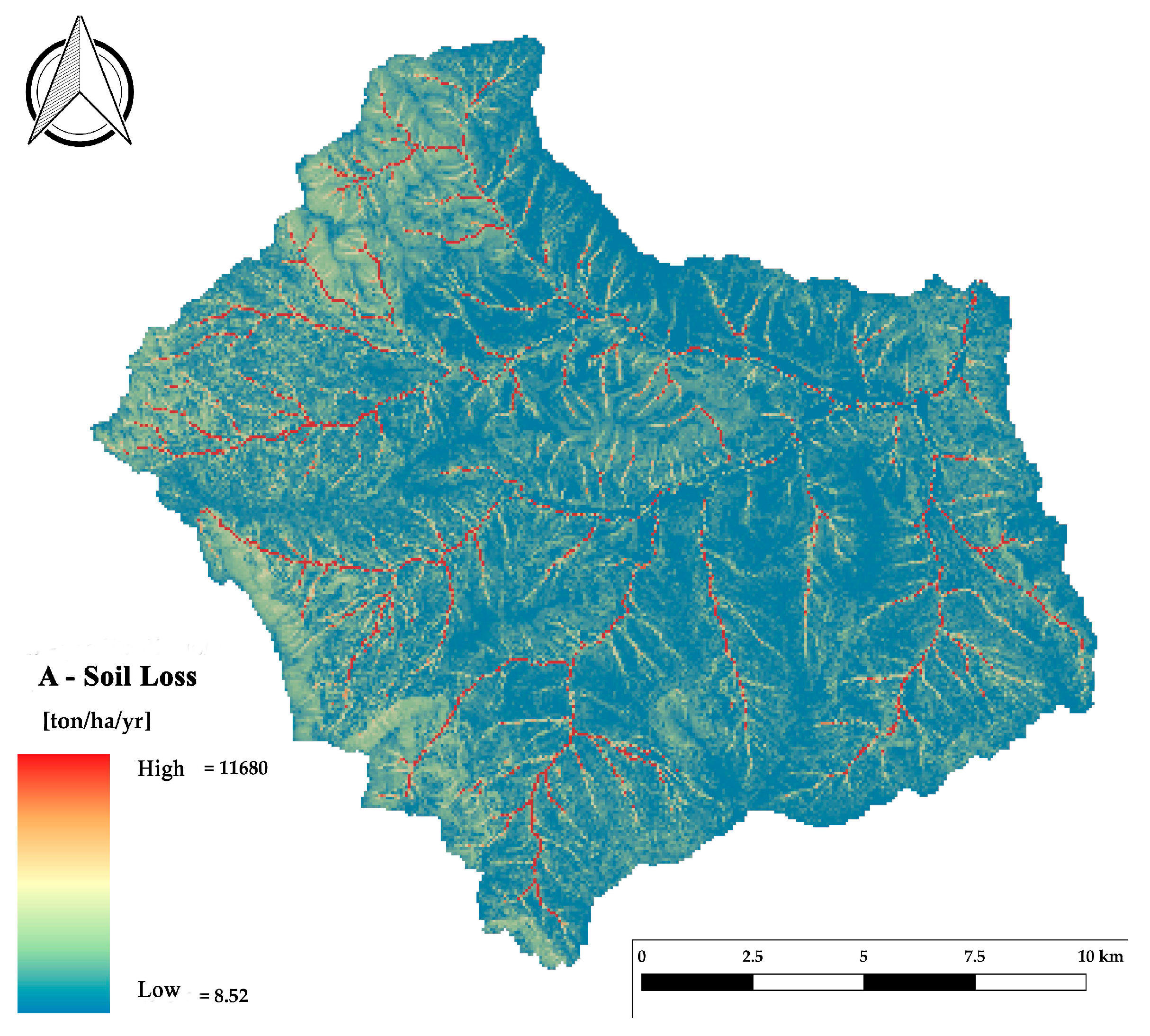
By multiplying the raster maps of all the factors previously obtained, the evaluation of the average annual soil loss A was carried out as shown in the following Figure 8.
Then by importing the raster file containing the average annual soil loss in GRASS it was possible to calculate the univariate statistics of the non-null pixels of the map. These statistics include the number of pixels counted, their minimum and maximum values, range width, arithmetic mean, population variance, standard deviation, coefficient of variation, and sum. All data are reported in Table 3.
These parameters show how the average value of annual erosion is equal to 71.4 ton/ha/year, that is fundamental to estimate the total amount of eroded soil in the basin, which is equal to 1,853,981 tons per year. This value is comparable, but more cautious than the value obtained in previous works [50] in which the LS-Factor does not take into account the mutual interaction of solid particles, in terms of path and confluences (see Table 4), providing a lower value of annual soil erosion. In fact, the annual soil loss is highly influenced by LS factor, then it is important that this factor could be estimated accurately [51,52]. Moreover, the value of eroded soil obtained in this work corresponds to 975,779 m3/year (concerning an average specific weight equal to 1900 kg/m3) or rather 3.758 mm/year, that is a value comparable with the average values of erosion in a basin like Camastra.
Then, the SDR of the Camastra Basin was carried out starting from the differences of several bathymetric surveys carried out for the homonymous reservoir (see Table 5) (provided by Agency for Development of Irrigation and Land Transformation in Puglia, Lucania, and Irpinia Area, in Italian: Ente per lo Sviluppo dell’Irrigazione e la Trasformazione Fondiaria in Puglia, in Lucania e in Irpinia), through which it was possible to calculate the average sedimented volume.
In particular, in addition to the data relating to the construction (1967) and commissioning (1988) of the reservoir, data were found on five bathymetric surveys conducted over a period of 25 years, from 1993 to 2017, thanks to an agreement between the Department of Engineering and Physics of the Environment (Dipartimento di Ingegneria e Fisica dell’Ambiente) of the University of Basilicata and Acqua S.p.A., a Company for the water supply of Basilicata, for the preparation of a feasibility study of a pilot project about the desilting of the Camastra Reservoir. Is important to highlight that after a critical analysis of the GIS calculations, it was considered possible to certify that the erosive phenomenon, represented by the average annual soil loss estimated with the model, is significantly influenced by the LS-Factor, which follows its pattern. This statement is also supported by the trend of surface flow accumulation, one of the module GRASS ‘r.watershed’© output, where in fact the pixels with a larger contributing area are those corresponding to the hydrographic network.
Moreover, by extrapolating these data up to now it has been possible to derive the current value of net erosion in reservoir, about 87,000 m3/yr [34,36], as well as the resulting annual average value of S.D.R. of the basin, which was equal to 0.082. In addition, the value of SDR was found to be reasonable with the values of mountainous watersheds like Camastra Basin [53].

3.2. The Risk Related to Soil Erosion

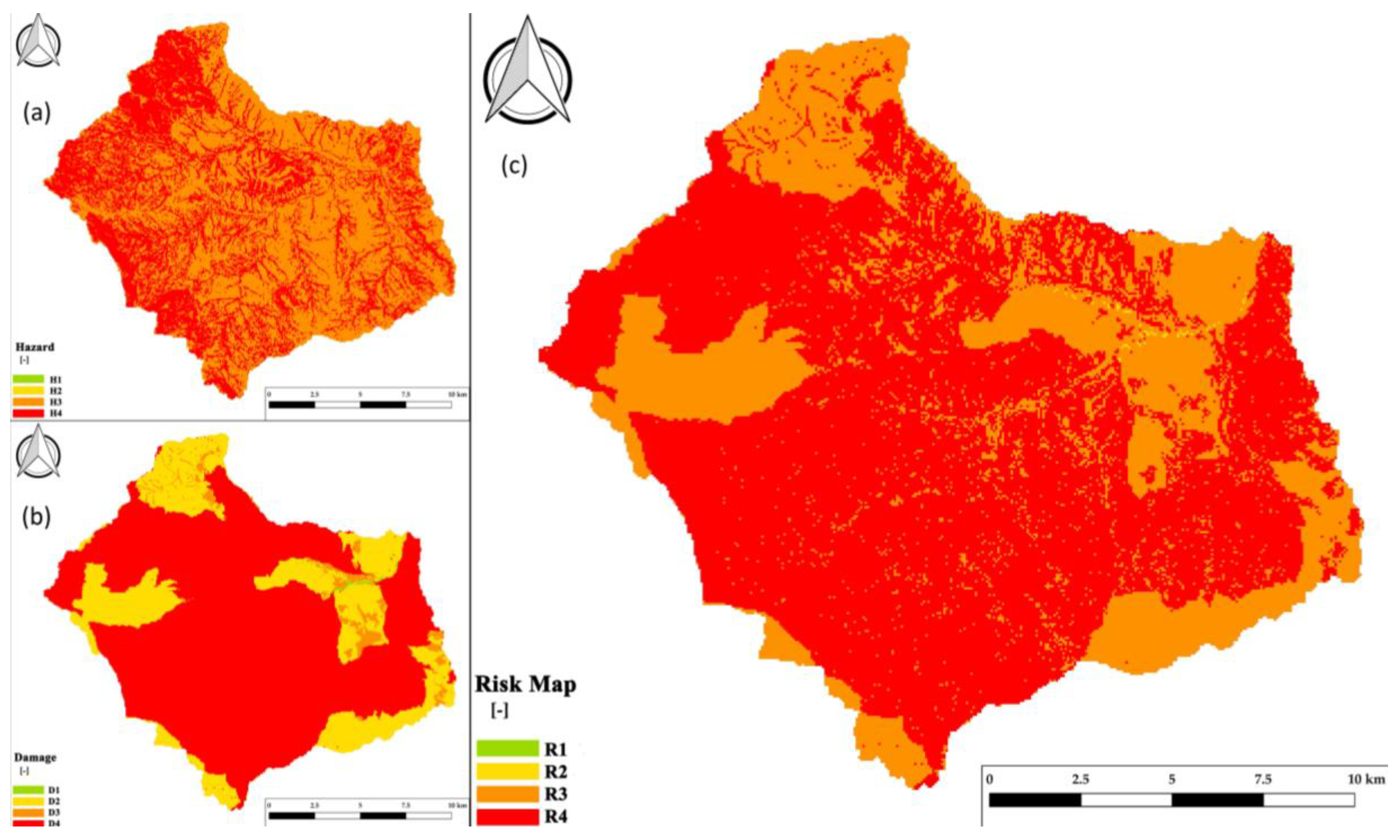
As seen in the previous section, the erosive phenomenon is high and distributed in a rather heterogeneous way over the whole basin, so it will probably be necessary to adopt extensive anti-erosive practices to reduce its severity. In particular, the Risk related to soil erosion can be assessed analytically, as a variable depending on the product between its Hazard (H) and Damage (D) [54]. In particular, a Hazard map serves as a cognitive framework of the territory that should be protected and is drawn up on the basis of an event scenario, (e.g., on the prior evaluation of the characteristics of a significant event). The magnitude of the event is expressed both in terms of the extent of the concerned area and through the parameters of intensity that characterize the scenario. Consequently, in this work the Hazard coincides with the average annual soil loss (A) evaluated with the method described above. Following the indications of the normative (D.Lgs.180/98 Italian Regulation), the criteria with which to establish the different levels of hazard have been established, and therefore the A-values have been grouped into four classes (see Figure 9a).
The Damage, on the other hand, being a function of the exposed resources, depends on the presence of human lives and the type of culture. To assess the Damage, factors have been sought that represent the exposed resources with parameters that can be quantified analytically, so as to impose their interaction through technical-scientific criteria. In detail, the data on land use and the ISTAT data of the last census were found in order to spatialize both the types of crops present and the number of inhabitants of the area of interest. For land use, the types of crops from the first level of the Corine land cover classification were grouped together while, for the ISTAT census sections, the minimum damage (D1) in the absence of inhabitants and the maximum damage (D4) for the inhabited sections were assumed. In particular, the highest priority is the population. Therefore, the damage of land use has been considered only where there are not inhabitants. Then, after rasterizing of layers of each single thematic map (land use and number of inhabitants), the final damage map was obtained by QGIS™ ‘raster calculator’© (see Figure 9b).
The Hazard and Damage values for each pixel in the basin were known and the corresponding Risk map could be developed (see Figure 9c).
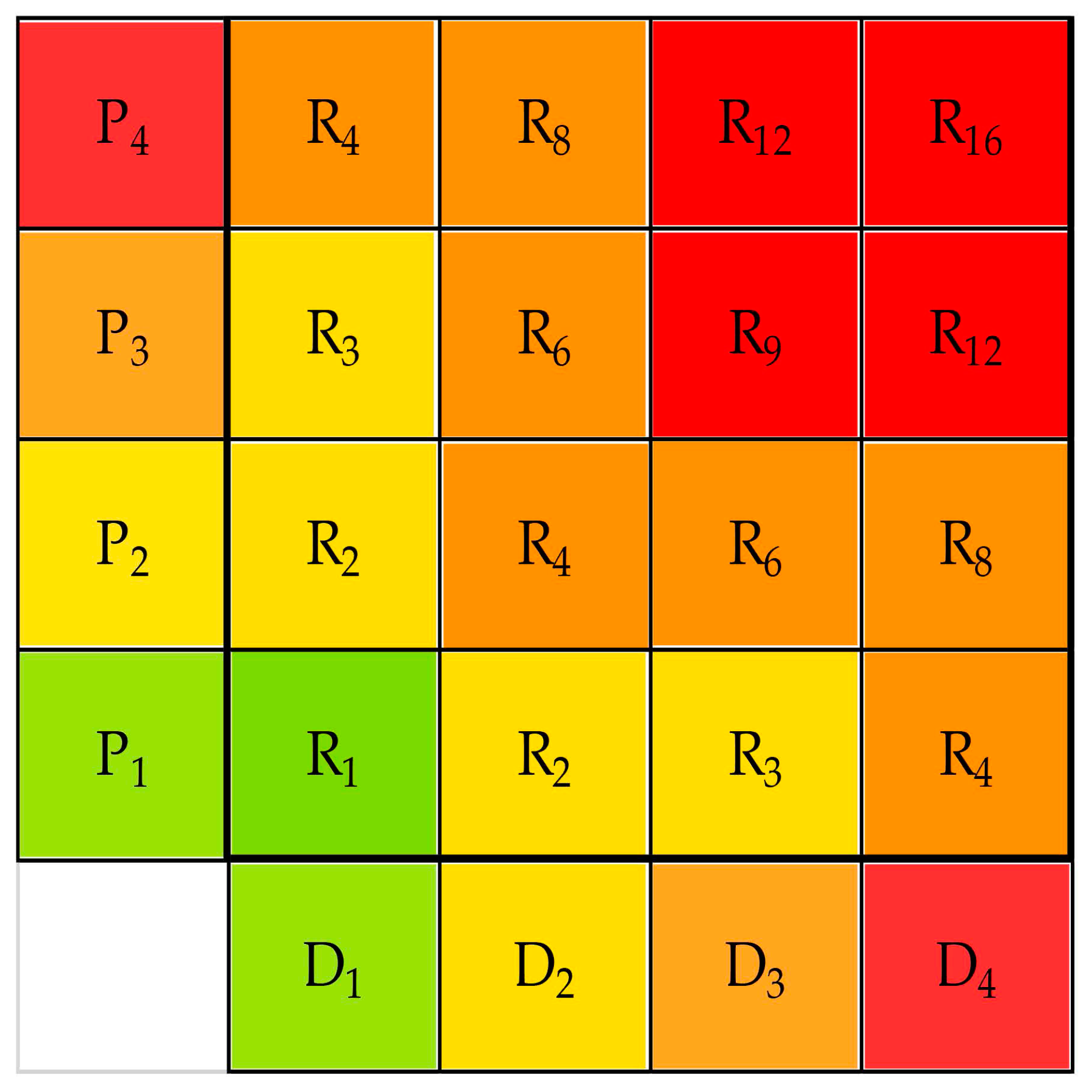
Of course, since both fields of values belong to the interval (1; 4), the initial domain of the Risk map coincides with the interval (1; 16). In order to standardize the result according to what is reported by the current norms, it was necessary to proceed to a further reclassification, inferable from the Risk matrix in Figure 10. In particular, the Italian Regulation 267/98 show the following four classes of risk: R1 ‘Moderate Risk’, low socioeconomic and environmental damages; R2 ‘Medium Risk’, minor damages to buildings, to infrastructures, to environmental heritage, without damages to people, to usability of buildings, and to economic activities; R3 ‘High Risk’, minor damages to people and functional damages to buildings, to infrastructures, to environmental heritage; R4 ‘Very High Risk’, serious injury to people, severe damages to buildings, to infrastructures, to environmental heritage, destruction of socioeconomic activities.

4. Conclusions

The revisitation of the factors of the RUSLE model addressed in this study, has provided very accurate results for the case under consideration, extendable to the entire Italian national territory. The improvements focused on the LS-Factor, initially the most critical parameter to be identified, but also the most important parameter in the estimation of soil loss due to erosion.
Moreover, the analysis carried out in GIS environment has allowed, despite the problems of accessibility and reliability of data, to implement a solid basis of the algorithm, which is also equipped with reproducibility, because as it was structured is totally independent of the case study.
In particular, the value of LS-Factor is comparable, but more cautious, than the value obtained in other works. This showed the importance for the topographic factor LS to take into account the mutual interaction of solid particles, in terms of path and confluences.
Finally, the model allows an effective estimate of the hydrological risk which, unlike the frequently proposed models [28,55,56,57,58,59,60,61,62,63,64,65], does not coincide with the only hazard associated with the phenomenon, but also considers the exposed resources. On the contrary, this modification has made it possible to highlight the most critical aspects of a territory in accordance with the political-economic strategies put in place by the competent Authorities and, at the same time, to verify in what way the introduction of a change in the management criteria adopted could modify the results.
Then, the use of the distributed approach described above, able to identify spatially and temporally the disruption due to water erosion, should be an integral part of any hydrogeological and hydraulic risk analysis, as it is essential to provide cognitive elements for the hydraulic protection of the territory. Extending the method to larger scales would make it possible to identify and quantify the main soil erosion factors in the various parts of the Country, to aid decision-makers and stakeholders on land management, environmental monitoring and prevention, and protection from overaggradation phenomena.

Author Contributions

Conceptualization, C.C.; data curation, L.C.; methodology, C.C.; software, D.N.P.; supervision, B.M.; validation, D.P.; writing—original draft, D.N.P.; writing—review and editing, L.C. All authors have read and agreed to the published version of the manuscript.

Funding

This research received no external funding.

Acknowledgments

The authors wish to thank the Ing. Vincenzo Savastano for his contribution and constructive comments and they recognize valuable input from the Ente per lo Sviluppo dell’Irrigazione e la Trasformazione Fondiaria in Puglia. Moreover, the authors thanks to the Civil Defense Office of Basilicata Region for rainfall data and NASA for spectral images.

Conflicts of Interest

The authors declare no conflict of interest.

Appendix A

The identification of the watershed of Camastra River derived from the geo-topographic database (http://rsdi.regione.basilicata.it/dbgt-ctr/) owned by the Basilicata Region, from which several metadata can be obtained, such as the Digital Elevation Model (DEM), land use maps, cadastral maps, topographic maps, and orthophotos. This database allows the download of different shapefiles in ESRI format both referring to the entire region and to the single municipality. Moreover, rainfall data were obtained from the Civil Defense Office (Protezione Civile) of Basilicata Region website (http://centrofunzionalebasilicata.it/it/), while the spectral images were acquired from the high temporal resolution spectroradiometer MODIS installed on NASA’s Landsat 8 satellite (LC08_L1TP_188032_20130706_20170503_01_T1).

References

  1. Jiu, J.; Wu, H.; Sen, L.S. The implication of land-use/land-cover change for the declining soil erosion risk in the Three Gorges Reservoir Region, China. Int. J. Environ. Res. Public Health 2019, 16, 1856. [Google Scholar] [CrossRef] [Green Version]
  2. Mohammad, R.; Ommolbanin, B.; Thomas, P.; Elham, R.S. Modeling the impact of climate change and land use change scenarios on soil erosion at the Minab Dam Watershed. Sustainability 2019, 11, 3353. [Google Scholar]
  3. Sujatha, E.R.; Sridhar, V. Spatial Prediction of Erosion Risk of a small mountainous watershed using RUSLE: A case-study of the Palar Sub Watershed in Kodaikanal, South India. Water 2018, 10, 1608. [Google Scholar] [CrossRef] [Green Version]
  4. Woldemariam, G.W.; Iguala, A.D.; Tekalign, S.; Reddy, R.U. Spatial modeling of soil erosion risk and its implication for conservation planning: The case of the Gobele Watershed, East Hararghe Zone, Ethiopia. Land 2018, 7, 25. [Google Scholar] [CrossRef] [Green Version]
  5. Bennett, H.H. Elements of Soil Conservation; McGraw-Hill Book Company Inc.: New York, NY, USA, 1955. [Google Scholar]
  6. Cencetti, C.; De Rosa, P.; Fredduzzi, A.; Marchesini, I. Erosione dei suoli e GRASS GIS: Esempi di applicazione. Geomat. Workb. 2005, 5, 16. (In Italian) [Google Scholar]
  7. De Vincenzo, A.; Molino, B.; Viparelli, R.; Caramuscio, P. A methodological approach for estimating turbidity in a river. Int. J. Sediment Res. 2011, 26, 112–119. [Google Scholar] [CrossRef]
  8. Bosco, C.; de Rigo, D.; Dewitte, O.; Poesen, J.; Panagos, P. Modelling soil erosion at European scale: Towards harmonization and reproducibility. Nat. Hazards Earth Syst. Sci. 2015, 15, 225–245. [Google Scholar] [CrossRef] [Green Version]
  9. Panagos, P.; Van Liedekerke, M.; Jones, A.; Montanarella, L. European Soil Data Centre: Response to European policy support and public data requirements. Land Use Policy 2012, 29, 329–338. [Google Scholar] [CrossRef]
  10. Panagos, P.; Borrelli, P.; Poesen, J.; Ballabio, C.; Lugato, E.; Meusburger, K.; Montanarella, L.; Alewell, C. The new assessment of soil loss by water erosion in Europe. Environ. Sci. Policy 2015, 54, 438–447. [Google Scholar] [CrossRef]
  11. Terranova, O.; Antronico, L.; Coscarelli, R.; Iaquinta, P. Soil erosion risk scenarios in the Mediterranean environment using RUSLE and GIS: An application model for Calabria (southern Italy). Geomorphology 2009, 112, 228–245. [Google Scholar] [CrossRef]
  12. Cook, H.L. The Nature and Controlling Variables of the Water Erosion Process. Soil Sci. Soc. Am. J. 1937, 1, 487–494. [Google Scholar] [CrossRef]
  13. Zingg, A.W. Degree and length of land slope as it affects soil loss in runoff. Agric. Eng. 1940, 21, 59–64. [Google Scholar]
  14. Smith, D.D. Interpretation of soil conservation data for field use. Agric. Eng. 1941, 22, 173–175. [Google Scholar]
  15. Renard, K.G.; Foster, G.R.; Weesies, G.A.; McCool, D.K.; Yoder, D.C. Predicting soil erosion by water: A guide to conservation planning with the Revised Universal Soil Loss Equation (RUSLE). In Agricultural Handbook; United States Department of Agriculture: Washington, DC, USA, 1997. [Google Scholar]
  16. Pandey, A.; Himanshu, S.K.; Mishra, S.K.; Singh, V.P. Physically based soil erosion and sediment yield models revisited. Catena 2016, 147, 595–620. [Google Scholar] [CrossRef]
  17. Morgan, R.P.C.; Nearing, M.A. Handbook of Erosion Modelling; Blackwell Publishing Ltd.: Chichester, UK, 2011. [Google Scholar]
  18. Capolongo, D.; Diodato, N.; Mannaerts, C.M.; Piccarreta, M.; Strobl, R.O. Analyzing temporal changes in climate erosivity using a simplified rainfall erosivity model in Basilicata (southern Italy). J. Hydrol. 2008, 356, 119–130. [Google Scholar] [CrossRef]
  19. Wischmeier, W.H. A Rainfall Erosion Index for a Universal Soil-Loss Equation. Soil Sci. Soc. Am. J. 1959, 23, 246–250. [Google Scholar] [CrossRef]
  20. Chaplot, V.; Saleh, A.; Jaynes, D.B.; Arnold, J. Predicting water, sediment and NO 3-N loads under scenarios of land-use and management practices in a flat watershed. Water Air Soil Poll. 2004, 154, 271–293. [Google Scholar] [CrossRef]
  21. Chaplot, V. Impact of spatial input data resolution on hydrological and erosion modeling: Recommendations from a global assessment. Phys. Chem. Earth 2014, 67, 23–35. [Google Scholar] [CrossRef]
  22. Wischmeier, W.H.; Smith, D.D. Predicting rainfall erosion losses—A guide to conservation planning. In Agricultural Handbook; United States Department of Agriculture: Washington, DC, USA, 1978. [Google Scholar]
  23. Williams, J.R. Sediment-yield prediction with Universal Equation using runoff energy factor. In Present and Prospective Technology for Predicting Sediment Yields and Sources; Agricultural Research Service, United States Department of Agriculture: Washington, DC, USA, 1975. [Google Scholar]
  24. Renard, K.G.; Foster, G.R.; Weesies, G.A.; Porter, J.P. RUSLE: Revised Universal Soil Loss Equation, Soil and Water Conservation Society. J. Soil Water Conserv. 1991, 46, 30–33. [Google Scholar]
  25. Mitasova, H.; Hofierka, J.; Zlocha, M.; Iverson, L.R. Modelling topographic potential for erosion and deposition using GIS. Int. J. Geogr. Inf. Syst. 1996, 10, 629–641. [Google Scholar] [CrossRef]
  26. Kinnell, P.I.A.; Risse, L.M. USLE-M: Empirical Modeling Rainfall Erosion through Runoff and Sediment Concentration. Soil Sci. Soc. Am. J. 1998, 62, 1667. [Google Scholar] [CrossRef]
  27. Nearing, M.A.; Romkens, M.J.M.; Norton, L.D.; Stott, D.E.; Rhoton, F.E.; Laflen, J.M.; Flanagan, D.C.; Alonso, C.V.; Binger, R.L.; Dabney, S.M.; et al. Measurements and models of soil loss rates. Science 2000, 290, 1300–1301. [Google Scholar] [CrossRef]
  28. Andreoli, R. Modeling Erosion Risk Using the RUSLE Equation. In QGIS and Applications in Water and Risks; Baghdadi, N., Mallet, C., Zribi, M., Eds.; John Wiley & Sons, Inc.: Hoboken, NJ, USA, 2018. [Google Scholar]
  29. Beskow, S.; Mello, C.R.; Norton, L.D.; Curi, N.; Viola, M.R.; Avanzi, J.C. Soil erosion prediction in the Grande River Basin, Brazil using distributed modeling. Catena 2009, 79, 49–59. [Google Scholar] [CrossRef]
  30. Irvem, A.; Topaloglu, F.; Uygyr, V. Estimating spatial distribution of soil loss over Seyhan River Basin in Turkey. J. Hydrol. 2009, 336, 30–37. [Google Scholar] [CrossRef]
  31. Shi, Z.H.; Cai, C.F.; Ding, S.W.; Wang, T.W.; Chow, T.L. Soil conservation planning at the small watershed level using RUSLE with GIS: A case study in the Three Gorge Area of China. Catena 2004, 55, 33–48. [Google Scholar] [CrossRef]
  32. Zhang, H.; Yang, Q.; Li, R.; Liu, Q.; Moore, D.; He, P.; Ritsema, C.J.; Geissen, V. Extension of a GIS procedure for calculating the RUSLE equation LS factor. Comput. Geosci. 2013, 52, 177–188. [Google Scholar] [CrossRef]
  33. Carone, M.T.; Greco, M.; Molino, B. A sediment-filter ecosystem for reservoir rehabilitation. Ecol. Eng. 2006, 26, 182–189. [Google Scholar] [CrossRef]
  34. De Vincenzo, A.; Molino, A.J.; Molino, B.; Scorpio, V. Reservoir rehabilitation: The new methodological approach of Economic Environmental Defence. Int. J. Sediment Res. 2017, 32, 288–294. [Google Scholar] [CrossRef]
  35. De Vincenzo, A.; Covelli, C.; Molino, A.; Pannone, M.; Ciccaglione, M.; Molino, B. Long-Term Management Policies of Reservoirs: Possible Re-Use of Dredged Sediments for Coastal Nourishment. Water 2018, 11, 15. [Google Scholar] [CrossRef] [Green Version]
  36. Molino, B.; Viparelli, R.; De Vincenzo, A. Effects of river network works and soil conservation measures on reservoir siltation. Int. J. Sediment Res. 2007, 22, 273. [Google Scholar]
  37. Molino, B.; De Vincenzo, A.; Ferone, C.; Messina, F.; Colangelo, F.; Cioffi, R. Recycling of clay sediments for geopolymer binder production. A new perspective for reservoir management in the framework of Italian legislation: The Occhito reservoir case study. Materials 2014, 7, 5603–5616. [Google Scholar] [CrossRef] [PubMed]
  38. Molino, B.; Savastano, V. Approccio distribuito per la stima dell’erosione idrica superficiale di un bacino idrografico, Il processo di interrimento degli invasi: Genesi, effetti ed interventi per la tutela dell’ambiente. Collana Stud. Ric. Dell’autorità Bacino Della Basilicata 2004, 4, 11–20. [Google Scholar]
  39. Onori, F.; De Bonis, P.; Grauso, S. Soil erosion prediction at the basin scale using the revised universal soil loss equation (RUSLE) in a catchment of Sicily (southern Italy). Environ. Geol. 2006, 50, 1129–1140. [Google Scholar] [CrossRef]
  40. Wu, L.; Liu, X.; Ma, X. Research progress on the watershed sediment delivery ratio. Int. J. Environ. Stud. 2017. [Google Scholar] [CrossRef]
  41. Renard, K.; Freimund, J. Using monthly precipitation data to estimate the Rfactor in the Revised USLE. J. Hydrol. 1994, 157, 287–306. [Google Scholar] [CrossRef]
  42. D’Asaro, F. Valutazione dell’indice di erosività relativo a singoli eventi erosivi. Riv. Ing. Agrar. 1994, XXV, 83–96. (In Italian) [Google Scholar]
  43. Rouse, J.W., Jr.; Haas, R.H.; Schell, J.A.; Deering, D.W. Monitoring the Vernal Advancement of Retrogradation of Natural Vegetation; NASA/GSFC: Greenbelt, MD, USA, 1974; Volume III, p. 371.
  44. Van der Knijff, J.; Jones, R.; Montanarella, L. Soil Erosion Risk: Assessment in Europe. In ISPRA: European Soil Bureau; Joint Research Centre: Ispra, Italy, 2000. [Google Scholar]
  45. McCool, D.K.; Foster, G.R.; Mutchler, C.K.; Meyer, L.D. Revised Slope Length Factor for the Universal Soil Loss Equation. Trans. ASAE 1989, 32, 1571–1576. [Google Scholar] [CrossRef]
  46. Ferro, V.; Porto, P.; Yu, B. A comparative study of rainfall erosivity estimation for southern Italy and southeastern Australia. Hydrol. Sci. J. 1999, 44, 3–24. [Google Scholar] [CrossRef]
  47. Mendicino, G.; Sole, A. Stima distribuita dell’erosione idrica lungo i versanti di un bacino sotteso da un invaso artificiale. In Proceedings of the Atti del XXVI Convegno di Idraulica e Costruzioni Idrauliche, Catania, Italy, 9–12 September 1998. (In Italian). [Google Scholar]
  48. Landsat 8 Satellite of NASA. 2017. Available online: https://www.nasa.gov/content/landsat-8-instruments (accessed on 5 April 2019).
  49. LULC of Basilicata Region. 2013. Available online: http://rsdi.regione.basilicata.it/ (accessed on 18 March 2019).
  50. Lazzari, M.; Gioia, D.; Piccarreta, M.; Danese, M.; Lanorte, A. Sediment yield and erosion rate estimation in the mountain catchments of the Camastra artificial reservoir (Southern Italy): A comparison between different empirical methods. Catena 2015, 127, 323–339. [Google Scholar] [CrossRef]
  51. Duarte, L.; Teodoro, A.C.; Gonçalves, J.A.; Soares, D.; Cunha, M. Assessing soil erosion risk using RUSLE through a GIS open source desktop and web application. Environ. Monit. Assess. 2016, 188, 351. [Google Scholar] [CrossRef] [PubMed]
  52. Yu, B.; Rosewell, C.J. Technical notes: A robust estimator of the R-factor for the universal soil loss equation. Trans. ASAE 1996, 39, 559–561. [Google Scholar] [CrossRef]
  53. Shi, Z.H.; Huang, X.D.; Ai, L.; Fang, N.F.; Wu, G.L. Quantitative analysis of factors controlling sediment yield inmountainous watersheds. Geomorphology 2014, 226, 193–201. [Google Scholar] [CrossRef]
  54. Canuti, P.; Casagli, N. Fenomeni Franosi e Centri Abitati. In Proceedings of the Conference of Bologna 1994 (CNR–GNDCI–Emilia-Romagna), Bologna, Italy, 27 May 1994; p. 66. (In Italian). [Google Scholar]
  55. Benchettouh, A.; Kouri, L.; Jebari, S. Spatial estimation of soil erosion risk using RUSLE/GIS techniques and practices conservation suggested for reducing soil erosion in Wadi Mina watershed (northwest, Algeria). Arab. J. Geosci. 2017, 10. [Google Scholar] [CrossRef]
  56. Bhattarai, R.; Dutta, D. Estimation of Soil Erosion and Sediment Yield Using GIS at Catchment Scale. Water Resour. Manag. 2007, 21, 1635–1647. [Google Scholar] [CrossRef]
  57. Demirci, A.; Karaburun, A. Estimation of soil erosion using R in a GIS framework: A case study in the Buyukcekmece Lake watershed, northwest Turkey. Environ. Earth Sci. 2012, 66, 903–913. [Google Scholar] [CrossRef]
  58. Gaubi, I.; Chaabani, A.; Mammou, A.B.; Hamza, M.H. A GIS-based soil erosion prediction using the Revised Universal Soil Loss Equation (RUSLE) (Lebna watershed, Cap Bon, Tunisia). Nat. Hazards 2017, 86, 219–239. [Google Scholar] [CrossRef]
  59. Haregeweyn, N.; Tsunekawa, A.; Poesen, J.; Tsubo, M.; Meshesha, D.T.; Fenta, A.A.; Nyssen, J.; Adgo, E. Comprehensive assessment of soil erosion risk for better land use planning in river basins: Case study of the Upper Blue Nile River. Sci. Total Environ. 2017, 574, 95–108. [Google Scholar] [CrossRef] [Green Version]
  60. Lu, D.; Li, G.; Valladares, G.S.; Batistella, M. Mapping soil erosion risk in Rondonia, Brazilian Amazonia: Using RUSLE, remote sensing and GIS. Land Degrad. Dev. 2004, 15, 499–512. [Google Scholar] [CrossRef]
  61. Moses, A. GIS-RUSLE Interphase Modelling of Soil Erosion Hazard and Estimation of Sediment Yield for River Nzoia Basin in Kenya. J. Remote Sens. GIS 2017, 6. [Google Scholar] [CrossRef]
  62. Singh, G.; Panda, R.K. Grid-cell based assessment of soil erosion potential for identification of critical erosion prone areas using USLE, GIS and remote sensing: A case study in the Kapgari watershed, India. Int. Soil Water Conserv. Res. 2017, 5, 202–211. [Google Scholar] [CrossRef]
  63. Weifeng, Z.; Bingfang, W.U. Assessment of soil erosion and sediment delivery ratio using remote sensing and GIS: A case study of upstream Chaobai River catchment, north China. Int. J. Sediment Res. 2008, 23, 167–173. [Google Scholar] [CrossRef]
  64. Winchell, M.F.; Jackson, S.H.; Wadley, A.M.; Srinivasan, R. Extension and validation of a geographic information system-based method for calculating the Revised Universal Soil Loss Equation length-slope factor for erosion risk assessments in large watersheds. J. Soil Water Conserv. 2008, 63, 105–111. [Google Scholar] [CrossRef]
  65. Farhan, Y.; Zregat, D.; Anbar, A. Assessing farmers’ perception of soil erosion risk in Northern Jordan. J. Environ. Prot. 2015, 6, 867. [Google Scholar] [CrossRef] [Green Version]
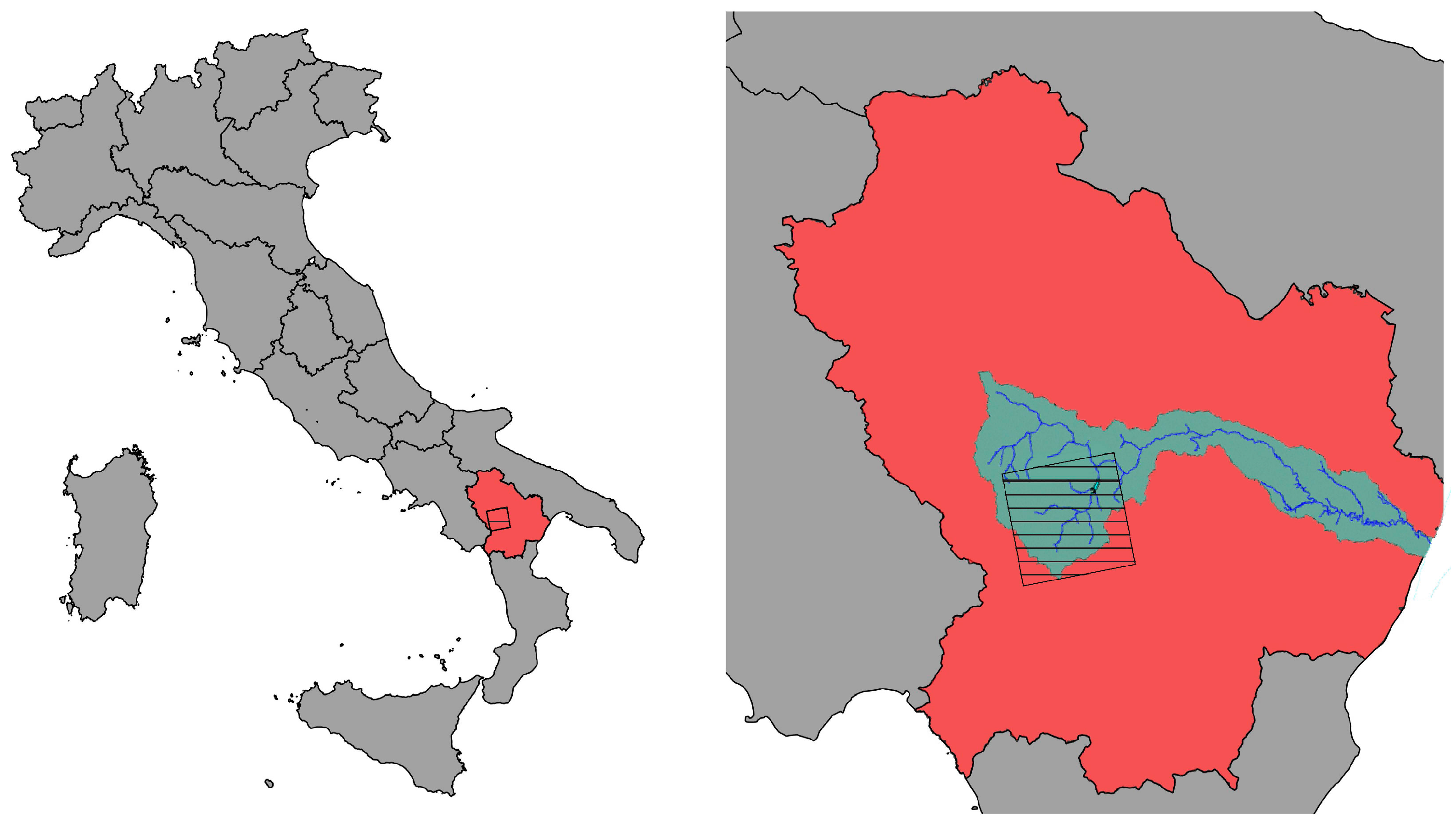
Figure 1. Basilicata region (red), Basento watershed (green), and Camastra basin (grid) (by QGIS).
Hydrology 07 00013 g001
Figure 2. Algorithm framework-flowchart: inputs, processes, and results integration.
Hydrology 07 00013 g002
Figure 3. Hypsographic curve.
Hydrology 07 00013 g003
Figure 4. Relief map: (a) by Google™ Earth Pro platform, (b) by QGIS™ software.
Hydrology 07 00013 g004
Figure 5. R-factor map.
Hydrology 07 00013 g005
Figure 6. C-Factor map.
Hydrology 07 00013 g006
Figure 7. Topographic factor: (a) LS-Factor map, (b) Length (L)-Factor map, (c) Slope (S)-Factor map.
Hydrology 07 00013 g007
Figure 8. Unit Soil Loss Equation map for the Camastra Basin based on Revised Universal Soil Loss Equation (RUSLE) model, in t/ha/yr.
Hydrology 07 00013 g008
Figure 9. The product between the hazard map (a) and the damage map (b) is the risk map (c).
Hydrology 07 00013 g009
Figure 10. Risk Matrix.
Hydrology 07 00013 g010
Table 1. QGIS™ location coordinates.
N-W15° 39′ 30,1204″ E40° 38′ 41,5553″ N
N-E16° 06′ 48,2343″ E40° 38′ 41,5553″ N
S-E16° 06′ 48,2343″ E40° 17′ 19,9166″ N
S-W15° 39′ 30,1204″ E40° 17′ 19,9166″ N
Table 2. Pluviographic data (mm).
Abriola
YearSept.Oct.Nov.Dec.Jan.Feb.Mar.Apr.MayJuneJulyAug.
2014/1569.848.475.045.4193.9203.6219.5112.555.999.620.563.1
2015/1664.3217.284.011.2124.5137.7244.668.7134.028.983.036.6
2016/17104.4133.3139.620.4149.047.8105.246.242.012.611.52.8
2017/18133.261.4192.8166.7147.0226.2237.662.3166.696.040.8130.5
Anzi
yearSept.Oct.Nov.Dec.Jan.Feb.Mar.Apr.MayJuneJulyAug.
2015/1625.8116.232.01.4117.979.877.78.415.833.4179.253.2
2016/17117.979.877.78.454.227.044.818.233.513.211.711.9
2017/1840.033.7109.533.443.691.061.639.4127.929.47.5130.5
Laurenzana
yearSept.Oct.Nov.Dec.Jan.Feb.Mar.Apr.MayJuneJulyAug.
2014/1571.239.272.256.6173.6177.2117.843.443.842.04.6104.8
2015/1642.8141.037.61.423.267.4236.637.876.049.662.278.2
2016/1780.676.4112.018.6127.841.064.218.243.435.819.813.6
2017/1860.625.2154.470.050.8180.8156.858.0142.249.83.859.0
Table 3. Univariate Statistics of Soil Loss raster map.
Not Null Cells68,436
Minimum value8.52
Maximum value11,680
Range11,671.4
Average71.4
Standard deviation168.9
Variance28,555.8
Variance Coeffcient236.70%
Sum4,885,374.9
Table 4. The average soil loss predicted by RUSLE for the Camastra drainage basin.
Authors(t yr−1)
Lazzari et al.1,677,378
Present study1,853,981
Table 5. Bathymetric surveys and solid inflow data in the reservoir.
YearInflow (106 m3)Yield (106 m3)
196735.1720
198828.7127
199321.7546.958
199520.7760.978
199721.1200.656
200519.4210.699
201718.4181.003