Doing Hydrology Backwards—Analytic Solution Connecting Streamflow Oscillations at the Basin Outlet to Average Evaporation on a Hillslope

Abstract

The concept of doing hydrology backwards, introduced in the literature in the last decade, relies on the possibility to invert the equations relating streamflow fluctuations at the catchment outlet to estimated hydrological forcings throughout the basin. In this work, we use a recently developed set of equations connecting streamflow oscillations at the catchment outlet to baseflow oscillations at the hillslope scale. The hillslope-scale oscillations are then used to infer the pattern of evaporation needed for streamflow oscillations to occur. The inversion is illustrated using two conceptual models of movement of water in the subsurface with different levels of complexity, but still simple enough to demonstrate our approach. Our work is limited to environments where diel oscillations in streamflow are a strong signal in streamflow data. We demonstrate our methodology by applying it to data collected in the Dry Creek Experimental Watershed in Idaho and show that the hydrology backwards principles yield results that are well within the order of magnitude of daily evapotranspiration fluctuations. Our analytic results are generic and they encourage the development of experimental campaigns to validate integrated hydrological models and test implicit parameterization assumptions.

1. Introduction

The concept of doing hydrology backwards, introduced in the literature in the last decade, relies on the possibility to invert the equations relating streamflow fluctuations at the catchment outlet to estimated hydrological forcings throughout the basin. Several papers have focused on recovering the precipitation forcing leading to large streamflow fluctuations (i.e., event hydrographs), however less attention has been given to recovering the forcing from evapotranspiration cycles during periods of no rain. An early research example that motivates hydrology in the backwards direction is the work in Reference [1], where the authors use time series of precipitation and streamflow at the basin outlet to estimate the spatial distribution of soil water deficit. A more recent study [2] employs the single assumption that streamflow is a function of subsurface storage, then proceeds to find time series for precipitation based solely on streamflow observations. In a follow up work [3] this line of research is continued by investigating the limitations and advantages of Kirchner’s method after studying many different hillslopes under various conditions. The authors of Reference [4] apply a similar strategy to the well-established relationship between soil moisture and precipitation. They use in situ and satellite data of soil moisture and invert the soil-water balance to describe the cumulative precipitation forcing that must occur. Additionally, the authors of Reference [5] use a data-based mechanistic modelling approach which involved identifying linear continuous-time transfer functions between streamflow and rainfall at sub-hourly precision. The possibility of inverting equations has been explored by the authors of Reference [6] to emphasize the distinction between parameter uncertainties and model-forcing uncertainties and they develop a Markov chain Monte Carlo method to recognize, and appropriately deal with, each type of uncertainty. Although less research on deducing evapotranspiration patterns from streamflow observations has been done, an example in this direction was conducted in Reference [7], which was interested in computing evapotranspiration using diurnal fluctuations in the groundwater table. They review various methods that demonstrate this concept while testing the accuracy of the methods.

When we do hydrology in the standard (forward) direction, we require some form of input values. This is usually precipitation, of which data is abundant, but has some uncertainty associated with it [8,9]. We also require some knowledge of the internal processes of the system, given in the form of a mathematical model, with the resulting output of runoff or streamflow. These outputs are easily observed and measured. When we reverse the process and do hydrology backwards, we still need an appropriate model, but in this case, we require output observations (streamflow at the outlet), which are often easier to obtain.

A strong motivation for developing inversion equations to do hydrology backwards is to provide modelers with additional mechanisms to validate hydrological models. For example, streamflow measurements are more likely to be available at the catchment scale than distributed measurements of runoff, soil moisture, precipitation or evapotranspiration at the much smaller hillslope scale. As a result, models that describe flows throughout the river network can easily compare output with streamflow observed data, but uncertainty remains regarding the internal dynamics in the basin. At the hillslope scale, rainfall-runoff models describe the pathways of precipitation into the river network as overland flow or through the subsurface via infiltration and subsurface flow. Although surface runoff observations are straightforward, direct observations of subsurface runoff are more complex. In addition, measurements of storage in the subsurface contain significant uncertainty due to heterogeneity in the soil [10]. Finally, the forcings to these rainfall-runoff models are precipitation and evapotranspiration. The former is frequently observed, while the latter must be computed using indirect observations (e.g., temperature, wind speed, relative humidity). The methodology of doing hydrology backwards provides a way to develop targeted small scale measurement campaigns that can help validate the modeling assumptions about flow travel pathways and residence times.

In this work, we use the concept of hillslope-link landscape decomposition described by Reference [11] to partition the basin area into small control volumes draining into the links of the river network. We assume that the full extent of the river network is preserved. This decomposition strategy has been used in previous modeling work and it is closely related to the the representative elementary watershed (REW) concept formulated by Reference [12]. We aim to test the feasibility of doing hydrology backwards by taking streamflow observations from a catchment under dry conditions and invert river network flow dynamics to infer the subsurface runoff at the hillslope scale. We then apply the hillslope subsurface runoff to invert an appropriate hillslope model to determine the evaporation forcing that must have occurred to create the corresponding subsurface runoff pattern.

The paper is organized as follows—In Section 2, we introduce the method we will use for hydrology backwards, beginning with a prescribed streamflow at the catchment scale and finding the hillslope runoff that produces it. The streamflow pattern is consistent with observed streamflows under dry conditions [13]. In Section 3, we use a simple subsurface model to begin the process of doing hydrology backwards at the hillslope scale. The process provides insight into the shortcomings of the subsurface model and suggests steps for improvement. Therefore, we introduce a more appropriate modified subsurface model. We use the latter in Section 4 to find the evapotranspiration forcing that produces the runoff pattern determined in Section 2. We apply these processes to the Dry Creek Experimental Watershed in Section 5. We offer concluding remarks in Section 6.

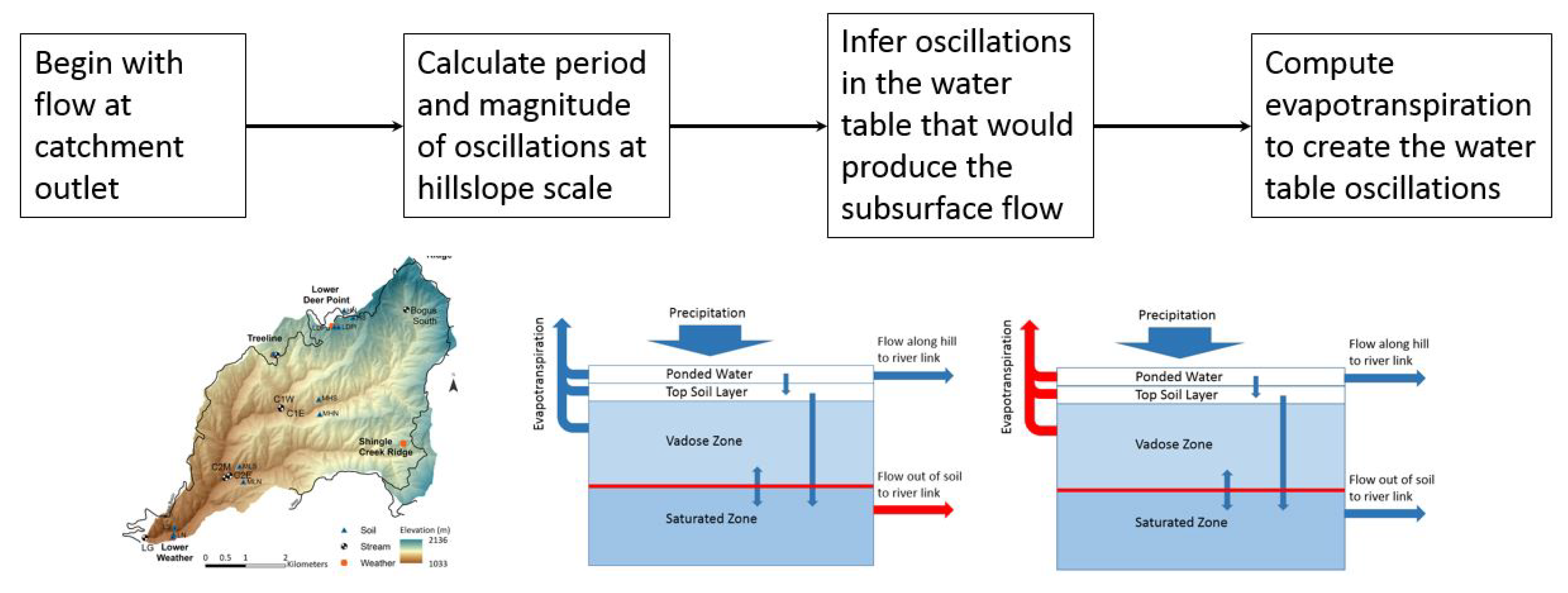
2. Hydrology Across Scales—Using Catchment Streamflow to Determine Hillslope Runoff

In order to ‘backtrack’ streamflow data to determine the runoff from each individual hillslope, we must make specific assumptions about precipitation, water movement through the river network and the spatial homogeneity of processes. We develop our methodology to detect diel fluctuations during periods of no precipitation. Diel fluctuations are less apparent during periods of high flows, since the dynamics of the streamflow are driven by surface runoff inputs. In a sense, the results of precipitation are present as storage in the saturated zone of soil. However, the model is not driven by precipitation during the analysis period. The river network is assumed to be composed of a finite number of interconnected links. We assume that water moves along each link in the river network at constant velocity, which gives a linear relationship between discharge and storage in the link, $q_i=\frac{v}{l}{s}_{c_i}$. In general, we do not expect significant variations of the velocity in the stream over the low flow periods that are the focus of this work. The resulting mass-balance equation was developed following the work in References [12,14,15,16], and is given by Equation (1):

$$\frac{d{q}_i\left(t\right)}{dt}=\frac{v}{l}(R\left(t\right)+q_{i1}\left(t\right)+q_{i2}\left(t\right)-q_i\left(t\right)),$$

(1)

where $q_i$ is the flow out of a given river link i, $q_{i1}$ and $q_{i2}$ are streamflows from the tributaries that connect at the upstream node of link i, $R\left(t\right)$ is runoff entering link i from the adjacent hillslope, v is the velocity in the river link, l is the length of the river link and $\frac{v}{l}$ is the transport constant, which is related to the residence time in the river link. Our assumption of constant velocity is well justified for periods of low flows where the changes in water levels in the channel are small over the time scales considered in this work (days). Equation (1) has been generalized to include nonlinear flows in the river network and has been implemented in the Iowa Flood Center flood forecasting system as described in Reference [17]. Additionally, the effects of this nonlinearity have been extensively studied in Reference [18].

We also assume that there is no surface runoff occurring in the catchment, that subsurface runoff is the same for all hillslopes and it takes the following form Equation (2):

$$R\left(t\right)=B{e}^{-At}+C{e}^{-At}sin\left(2\pi \nu t\right),$$

(2)

with A, B, C and $\nu$ are positive parameters with $C<B$ to ensure that the baseflow takes only positive values. This set of assumptions allows us to use the analytic solutions developed in Reference [19] to describe water movement through the river network. This equation does not account for rainfall, since realistic rainfall would not be well represented by an analytic function.

The inversion problem from outlet streamflow to hillslope runoff reduces to seeking values for the parameters A, B and C. We use the nonlinear curve-fitting software from MATLAB’s statistics package to identify appropriate parameter values. Inputs to the software include the explicit streamflow function and initial guesses for parameter values. We will demonstrate the numerical fitting results in Section 5.

3. Damping Oscillatory Runoff Patterns and Hillslope Scale Physical Processes

In this section we determine sufficient conditions for the water movement through the subsurface to produce a prescribed baseflow pattern. The subsurface requirements that we identify below are consistent with the findings of Reference [20] and allow for analysis and interpretation of the effects of soil type and plant life on baseflow.

We begin by using the assumption that water in the subsurface can be described by a linear model. Obviously, this formulation is a simplification of water dynamics at the hillslope level. However, our approach is acceptable as long as the linear model is capable of generating baseflow patterns comparable to those observed in links of realistic river networks.

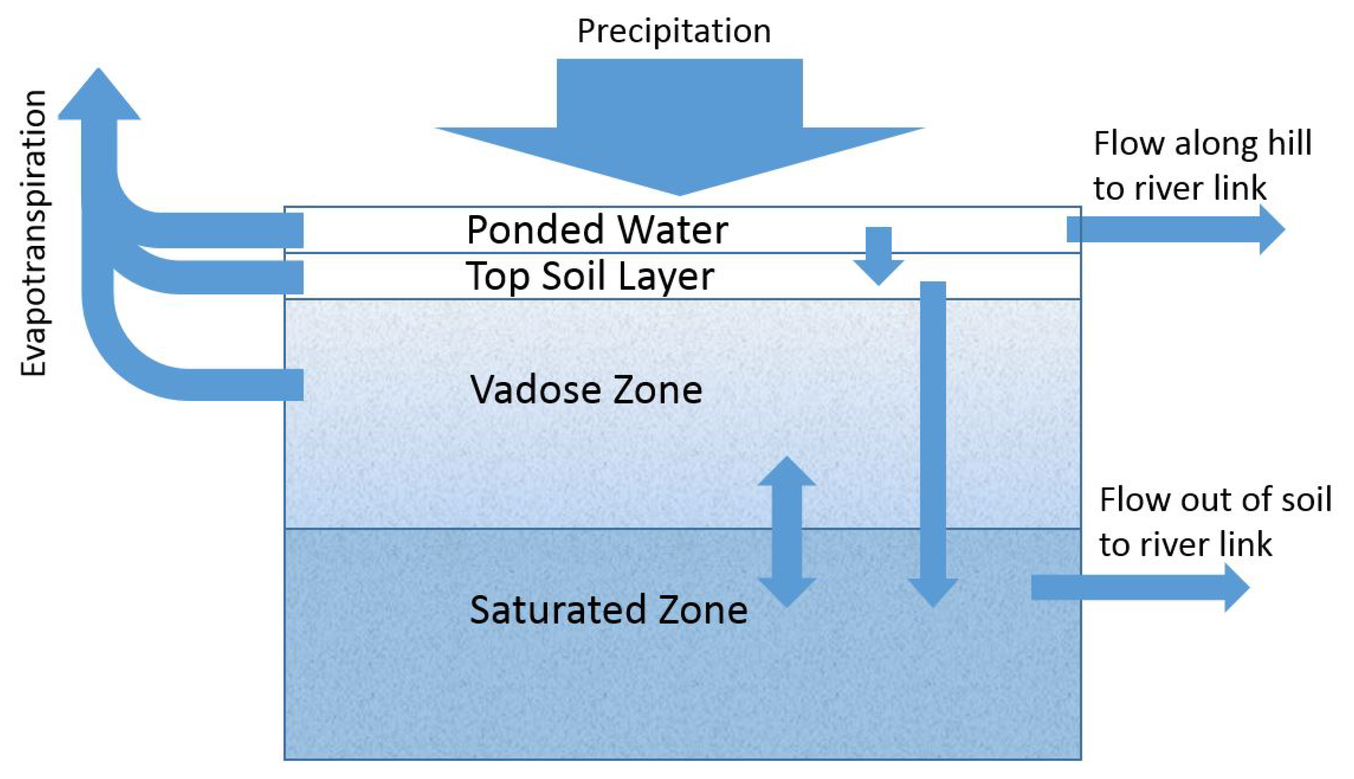
3.1. Model to Describe Water

To represent water movement through the subsurface at the hillslope scale, we follow the modelling techniques of Reference [21,22,23], which use conservation of mass to develop the following two-dimensional linear ordinary differential equation (ODE) model (Equation (3)):

$$\begin{array}{cc}\hfill \frac{d{s}_p}{dt}=& P{c}_1-k_2{s}_p-e_p\hfill \\ \hfill \frac{d{s}_s}{dt}=& P{c}_2-k_3{s}_s-e_s\hfill \end{array}$$

(3)

where the model variables are $s_p$, the volume of water ponded atop the hillslope and $s_s$, the volume of water in the subsurface. The inputs are P, the precipitation intensity and $e_p$ and $e_s$ which represent the evapotranspiration components from the ponded water and from the subsurface, respectively. The rates $k_2$ and $k_3$ are used to characterize the fluxes of infiltration and subsurface flow and are assumed to be constant. The parameters $c_1$ and $c_2$ serve two purposes. First, they convert the conventional units of precipitation to be consistent with the model. Secondly, they apply the runoff coefficient which determines the percentage of water that will become surface runoff and the remainder that will infiltrate into the subsurface.

Since we limited the scope of this work to situations in which subsurface flow is the dominant source of runoff we expect no ponded water to exist nor infiltration to occur. Thus, the equations describing surface runoff can be ignored and we can focus our attention on the second equation of system (Equation (3)), which can be rewritten as Equation (4):

$$\frac{d{s}_s}{dt}=q_{in}-k_3{s}_s-e_s$$

(4)

where $q_{in}$ is the incoming flux to the subsurface and $k_3{s}_s$ is water exiting as subsurface flow to the adjacent stream. Note that without ponded surface water, the hillslope will have no overland flow contributing to total runoff, so subsurface flow is the only runoff source.

Since Equation (4) is linear, it can be easily integrated, leading to a subsurface flow formulation ($k_3{s}_s$) defined by Equation (5):

$${\displaystyle k_3{s}_s=k_3{s}_{s0}{e}^{-k_{3}t}+e^{-k_{3}t}{\int }_0^t{k}_3{e}^{k_{3}u}[q_{in}\left(u\right)-e_s\left(u\right)]du.}$$

(5)

This formula is consistent with the observation that, under dry conditions (such as late summer), baseflow undergoes exponential decay as water drains from the hillslope (e.g., Reference [13]). In the case of fluctuating streamflow signals (as observed in many studies; for example, References [24,25]), we expect that the baseflow also exhibits an oscillatory pattern, though exponentially attenuated. Therefore, as a first step in our analysis, we will use Equation (5) to identify sufficient conditions on the forcing term ($q_{in}-e_s$) to produce exponentially decaying oscillatory patterns in the runoff.

3.2. Expected Subsurface Characteristics That Lead to Observed Fluctuating Runoff Patterns

Let us assume now that the total runoff from each hillslope to the river link in a given river basin is oscillatory and its amplitude undergoes exponential decay (as seen for baseflow under dry conditions). Then, we define the runoff by the formula Equation (6):

$$R\left(t\right)=B{e}^{-At}+C{e}^{-At}sin\left(2\pi \nu t\right),$$

(6)

with A, B, C and $\nu$ positive parameters and $C<B$ to ensure that the subsurface flow takes only positive values.

A sample subsurface runoff pattern with parameter values $A=0.003$ ($1/\mathrm{h}$), $B=0.08$ ($\mathrm{L}·{\mathrm{s}}^{-1}$), $C=0.008$ ($\mathrm{L}·{\mathrm{s}}^{-1}$) and $\nu =\frac{1}{24}$ [${\mathrm{h}}^{-1}$] is illustrated in Figure 1. The value of $\nu$ is chosen so that the frequency of the oscillations corresponds to a period of 24 h, representing a diurnal signal.

Since the runoff pattern R of Equation (6) must equal the subsurface runoff $k_3{s}_s$ of Equation (5) for any time t, the parameters A and $k_3$ need to be identical. Therefore A, the rate of decay of the subsurface flow signal has a physical meaning—it represents the linear rate at which water moves from the subsurface to the river link. A realistic value for this parameter is, for example, $A=1/340\approx 0.0001$ ($1/\mathrm{days}$), which was reported in previous work [26]. It would correspond to a type of soil that would take 340 days to drain to approximately $37\%$ of its initial value. Reasonable values of A vary depending upon soil type. Next, we get $B=k_3{s}_{s0}$, so the value of B represents the subsurface flow at time 0 and it can be directly estimated from data. The value of C can also be estimated from data as follows—once the rate of exponential decay (A) has been extracted, C will result as the amplitude of the oscillatory signal ($R{e}^{-At}$). Then, from the equality $R=k_3{s}_s$, we obtain ${\displaystyle Csin\left(2\pi \nu t\right)={\int }_0^{t}A{e}^{Au}(q_{in}\left(u\right)-e_s\left(u\right))du}$ or, by differentiation Equation (7):

$$q_{in}-e_s=\frac{2\pi \nu C}{A}{e}^{-At}cos\left(2\pi \nu t\right)$$

(7)

What can be said about $q_{in}$ and $e_s$ in Equation (7)? The assumption of dry conditions implies that $q_{in}$ is zero, causing evapotranspiration to attain negative values. This result implies that the simple formulation given in this section is not sufficient. To reconcile observations and our description of the physical processes in the subsurface, we reconsider the implicit assumption in our equations that flow into the unsaturated zone, $q_{in}$, comes only from precipitation. We employ the results of Reference [20] that reports that plants pull water from the subsurface during the day to meet the transpiration demand set forth by atmospheric conditions, but they reduce their pull during the night when the demand for transpiration wanes. As a consequence, the flux of water in the subsurface changes direction from being downward and driven by gravity at night to upward during the day. These results indicate that $q_{in}$, rather than being zero, should be defined by an oscillatory function which is positive (water being added to the subsurface) during the night and negative (water being removed from the subsurface) during the day (it will still be zero in its average, though). These observations motivate us to add one level of complexity to our subsurface storage equations to include the role of the unsaturated zone in the generation of subsurface runoff.

3.3. The Modified Hillslope Model

In this section, we modify the subsurface model given by Equation (3) so that it includes the results from Section 3.2 (oscillatory rather than zero flux $q_{in}$). Modifications include the addition of two subsurface layers. The top layer of subsurface receives infiltration from the ponded layer then transmits water to the saturated zone via preferential flow paths. The vadose (unsaturated) zone depicts the effects of vegetation, alternately pulling water from and releasing water to the saturated zone to maintain a soil moisture level set forth by evaporation demands. The saturated zone no longer includes an evapotranspiration term, but the subsurface flow remains the same.

The resulting hillslope model is a four dimensional set of ordinary differential equations (ODEs) given by Equation (8):

$$\begin{array}{cc}\hfill \frac{d{s}_p}{dt}=& P-Q_{pl}-Q_{pLink}-Eva{p}_p\hfill \\ \hfill \frac{d{s}_l}{dt}=& Q_{pl}-Q_{ls}-Eva{p}_l\hfill \\ \hfill \frac{d{s}_z}{dt}=& -Q_{sz}-Eva{p}_z\hfill \\ \hfill \frac{d{s}_s}{dt}=& Q_{ls}+Q_{sz}-Q_{sLink}.\hfill \end{array}$$

(8)

The variables of this system are $s_p$, $s_l$, $s_z$ and $s_s$, and they represent water ponded atop the hillslope surface, water in the top layer of subsurface, water in the vadose zone of subsurface and water in the saturated zone of subsurface, respectively. The system of equation is an extension of the equations used by Reference [17] to simulate flows in Iowa. The distinction between $s_l$ and $s_z$ is that water in the top layer of subsurface is near enough to the surface that it undergoes direct evaporation, while water in the vadose zone is deep enough that it cannot be evaporated. Instead water in the vadose zone is removed by plant roots to meet transpiration demands.

The fluxes that describe water movement through the system are defined and described in

Table 1. Flux formulas and descriptions for the ODE system (8).

Flux	Physical Meaning
$Q_{pl}=k_{dry}{s}_p{\left(1-\frac{s_l}{t_l}\right)}^3$	The flux from ponded water into the
	top layer of subsurface
$Q_{ls}=k_i{s}_l$	The flux from water in the top layer of
	subsurface to the saturated layer of subsurface
$Q_{sz}=50E{v}_{avg}{c}_1\left[\left(\frac{s_z}{b_L-s_s}-{\Theta }_R\right)\right]$	The flux between the vadose zone
	and the saturated zone
$Q_{pLink}=k_2{s}_p$	Overland flow from ponded water to
	river link
$Q_{sLink}=k_3{s}_s$	Flow from saturated subsurface to river link
${\Theta }_R=f\left(Evap\right)$	Soil moisture determined by evaporation

, and a visual depiction is given in Figure 2. Particular attention should be paid to $Q_{sz}$, the flux between the vadose zone of subsurface and the saturated zone of subsurface. This flux can describe flow in either direction and is, by convention, positive in the direction from the vadose zone to the saturated zone. The addition of the vadose zone and $Q_{sz}$ allow the gradient of water in the subsurface to have a downward direction during the night, when gravity is the dominant force, but an upward direction during the day, when plant life siphons water to meet the evapotranspiration demands. Both the direction and the magnitude of $Q_{sz}$ are designed to maintain a level of residual soil moisture in the unsaturated zone, so that ${\Theta }_R$ is included in the expression for $Q_{sz}$. The residual soil moisture level depends on the evaporation from the unsaturated zone, so it is given by a function $f\left(Eva{p}_z\right)$. To be more specific, this function should be increasing so that when water is removed from the unsaturated zone, it pulls water as needed from the saturated zone.

The evapotranspiration forcing consists of three components—$Eva{p}_p$, $Eva{p}_l$ and $Eva{p}_z$. They describe water removal from the ponded layer, top layer and vadose zone, respectively. Because these three components work to meet a fixed demand, they will contribute to evapotranspiration only when water is available in their corresponding compartment. This is enforced by the terms $C_r{C}_p$, $C_r{C}_l$ and $C_r{C}_z$, each of which is in the range (0,1). As an example, we will consider $C_r{C}_z$, relating to evapotranspiration from the vadose zone. If either (or both) the ponded or top layer contain water, then either (or both) of $C_p$ or $C_l$ is nonzero and $C_r{C}_z=\frac{C_z}{C_p+C_l+C_z}$ is less than 1. In this example only some portion of the total evapotranspiration demand is met by the vadose zone. On the other hand, if both $C_p$ and $C_l$ are zero because the ponded and top layers are dry, then $C_r{C}_z=1$ and all of the evapotranspiration demand must be met by the vadose zone. This example is of particular interest because we will consider dry conditions, wherein $C_p$ and $C_l$ are zero, so that $Eva{p}_z=c_{1}Evap$. The resulting formulas to describe evapotranspiration are described in

Table 2. Formulas to divide evaporation into components being contributed from each zone.

Expression	Physical Meaning
$Eva{p}_p=C_r{C}_{p}Evap$	Evaporation from the ponded water (m/min)
$Eva{p}_l=C_r{C}_{l}Evap$	Evaporation from the top layer of subsurface (m/min)
$Eva{p}_z=C_r{C}_{z}Evap$	Temperature-driven transpiration from the vadose zone
	(m/min)
$Evap=c_1\mathrm{Actual}\mathrm{Evaporation}$	Common units for evapotranspiration are (mm/h).
	We convert to (m/min) with the conversion factor
	$c_1=\frac{{10}^{-3}}{60}$
$C_r=\frac{1}{C_p+C_l+C_z}$	Divides the evapotranspiration into three portions
$C_p=s_p$	The proportion of evapotranspiration from the ponded
	water depends directly upon the amount of water in the
	ponded zone
$C_l=\frac{s_l}{T_L}$	The proportion of evapotranspiration from the top layer
	depends on the proportion of the top layer containing
	water
$C_z=\frac{s_z}{b_L-s_s}$	The proportion of evapotranspiration from the vadose
	zone depends on the proportion of the vadose zone
	containing water

.

Under dry conditions, the system of differential equations given by (8) can be simplified because there will be no ponded water or water in the top layer of subsurface. In this case, all of the following are zero— $s_p$, $s_l$, P, $Q_{pl}$, $Q_{pLink}$, $Eva{p}_p$, $Q_{ls}$ and $Eva{p}_l$. We can then focus our attention on the last two equations of (8), which are simplified to the following (Equation (9)):

$$\begin{array}{cc}\hfill \frac{d{s}_z}{dt}=& -Q_{sz}-Eva{p}_z\hfill \\ \hfill \frac{d{s}_s}{dt}=& Q_{sz}-Q_{sLink},\hfill \end{array}$$

(9)

which describes how the system drains.

4. Using the Subsurface Model and Subsurface Flow to Determine Evapotranspiration

In this section, we will use a general subsurface flow function to determine the forcing pattern of evapotranspiration that must be applied at the hillslope scale. Suppose first a general form of runoff $R\left(t\right)$. The corresponding term in the simplified model from Equation (9) is $Q_{sLink}$, whose expression using system variables is given in Table 1. Because runoff and subsurface storage are linearly related, we can find an expression for saturated subsurface storage in terms of runoff as $s_s=\frac{R\left(t\right)}{k_3}$ so $Q_{sLink}=R\left(t\right)$. Differentiating with respect to time, we develop a second differential equation for $s_s$ written in terms of $R^{\prime }$, which must be the same as the differential equation given in Equation (9). Equating the two, we see that $\frac{R^{\prime }\left(t\right)}{k_3}=Q_{sz}-R\left(t\right)$ and we can now describe the flux $Q_{sz}$ in terms of the observed streamflow pattern as

$$Q_{sz}=\frac{R^{\prime }\left(t\right)}{k_3}+R\left(t\right).$$

Furthermore, $Q_{sz}$ can be expressed in terms of the system variables, as seen in Table 1. We equate the two expressions and solve for $s_z$ in terms of runoff as

$$s_z=\left[\frac{1}{k_1}\left(\frac{R^{\prime }\left(t\right)}{k_3}+R\left(t\right)\right)+f\left(Eva{p}_z\right)\right]\left(b_L-\frac{R\left(t\right)}{k_3}\right),$$

where $k_1=50E{v}_{avg}{c}_1$ and $f\left(Eva{p}_z\right)$ is a function to represent residual soil moisture, ${\Theta }_R$. This is because under dry conditions, $Eva{p}_z=Evap$ (see also the definitions of ${\Theta }_R$ in Table 1). We again differentiate, and recognize that our two expressions from $s_z$ (one from differentiating the formula for $s_z$ and another from Equation (9)) must be the same, so that Equation (10):

$$\begin{array}{cc}\hfill & \left(\frac{1}{k_1{k}_3}{R}^{\prime }\left(t\right)+\frac{1}{k_1}R\left(t\right)+f\left(Eva{p}_z\right)\right)\left(\frac{-1}{k_3}{R}^{\prime }\left(t\right)\right)\hfill \\ \hfill & +\left(b_L-\frac{1}{k_3}R\left(t\right)\right)\left(\frac{1}{k_1{k}_3}{R}^{″}\left(t\right)+\frac{1}{k_1}{R}^{\prime }\left(t\right)+f^{\prime }\left(Eva{p}_z\right)\frac{dEva{p}_z}{dt}\right)\hfill \\ \hfill =& \frac{-1}{k_3}{R}^{\prime }\left(t\right)-R\left(t\right)-Eva{p}_z.\hfill \end{array}$$

(10)

We now reorganize Equation (10) to get the following differential equation in $Eva{p}_z$

$$\begin{array}{cc}\hfill \frac{dEva{p}_z}{dt}{f}^{\prime }\left(Eva{p}_z\right)=& \frac{-\frac{1}{k_3}{R}^{\prime }\left(t\right)-R\left(t\right)-Eva{p}_z+\frac{R^{\prime }\left(t\right)}{k_3}\left(\frac{1}{k_1{k}_3}{R}^{\prime }\left(t\right)+\frac{1}{k1}R\left(t\right)+f\left(Eva{p}_z\right)\right)}{b_L-\frac{1}{k_3}R\left(t\right)}\hfill \\ \hfill & -\frac{1}{k_1{k}_3}{R}^{″}\left(t\right)-\frac{1}{k_1}{R}^{\prime }\left(t\right).\hfill \end{array}$$

By grouping terms together, we can simplify the equation as an ODE for $Eva{p}_z$ as Equation (11):

$$\frac{dEva{p}_z}{dt}{f}^{\prime }\left(Eva{p}_z\right)=a_0(R,R^{\prime },R^{″})+a_1\left(R\right)Eva{p}_z+a_2(R,R^{\prime })f\left(Eva{p}_z\right),$$

(11)

where the coefficients $a_0(R,R^{\prime },R^{″})$, $a_1\left(R\right)$ and $a_2(R,R^{\prime })$ are given by Equation (12):

$$\begin{array}{cc}\hfill a_0=& \frac{1}{k_1{k}_3(k_3{b}_L-R)}\left[(R^{″}+k_3{R}^{\prime })(R-k_3{b}_L)+(R^{\prime }+k_{3}R)(R^{\prime }-k_1{k}_3)\right]\hfill \\ \hfill a_1=& \frac{-k_3}{k_3{b}_L-R}\hfill \\ \hfill a_2=& \frac{R^{\prime }}{k_3{b}_L-R}.\hfill \end{array}$$

(12)

We rewrite Equation (11) in terms of $w={\Theta }_R$, the residual soil moisture, as Equation (13):

$$\frac{dw}{dt}=a_0(R,R^{\prime },R^{″})+a_1\left(R\right)f^{-1}\left(w\right)+a_2(R,R^{\prime })w.$$

(13)

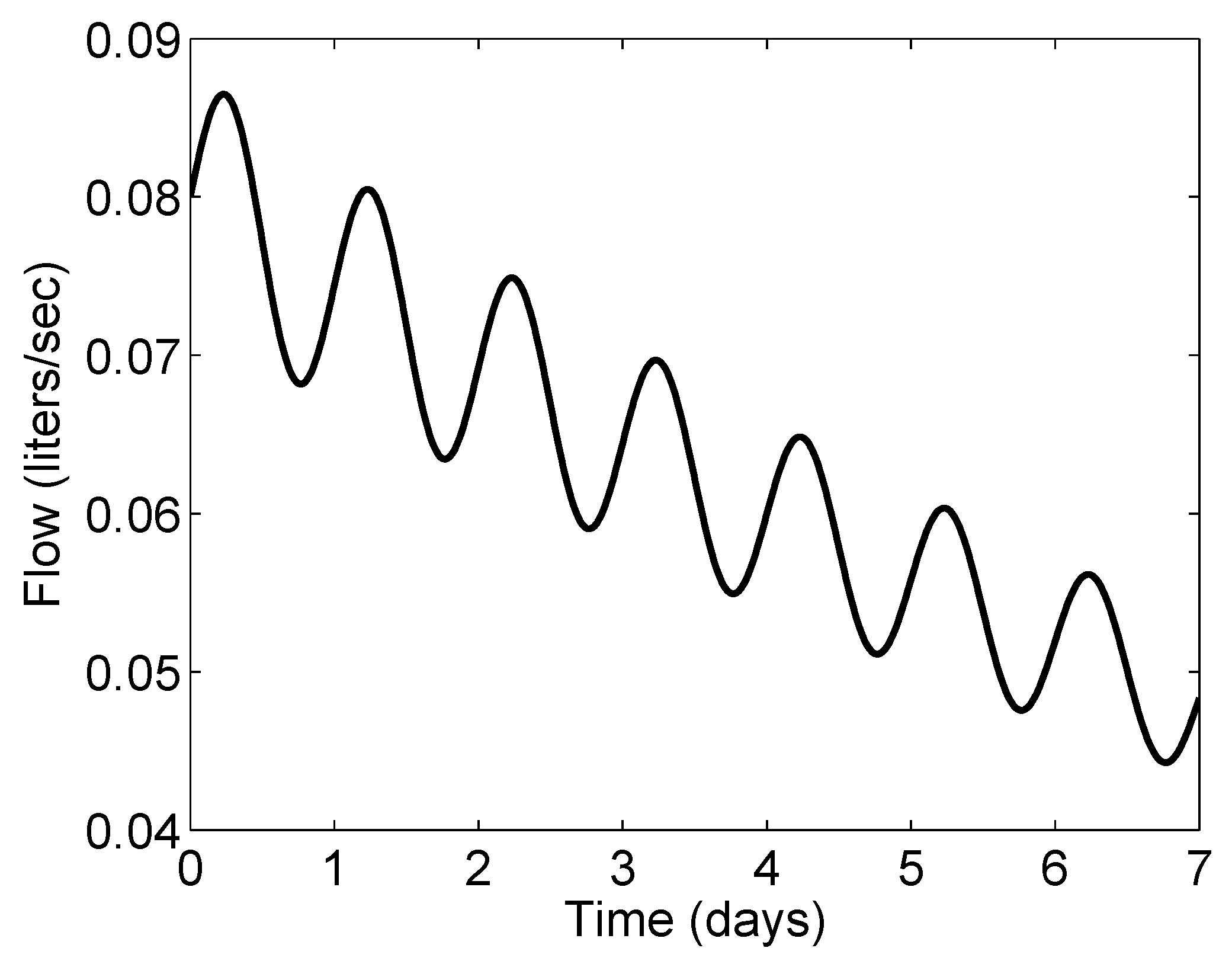
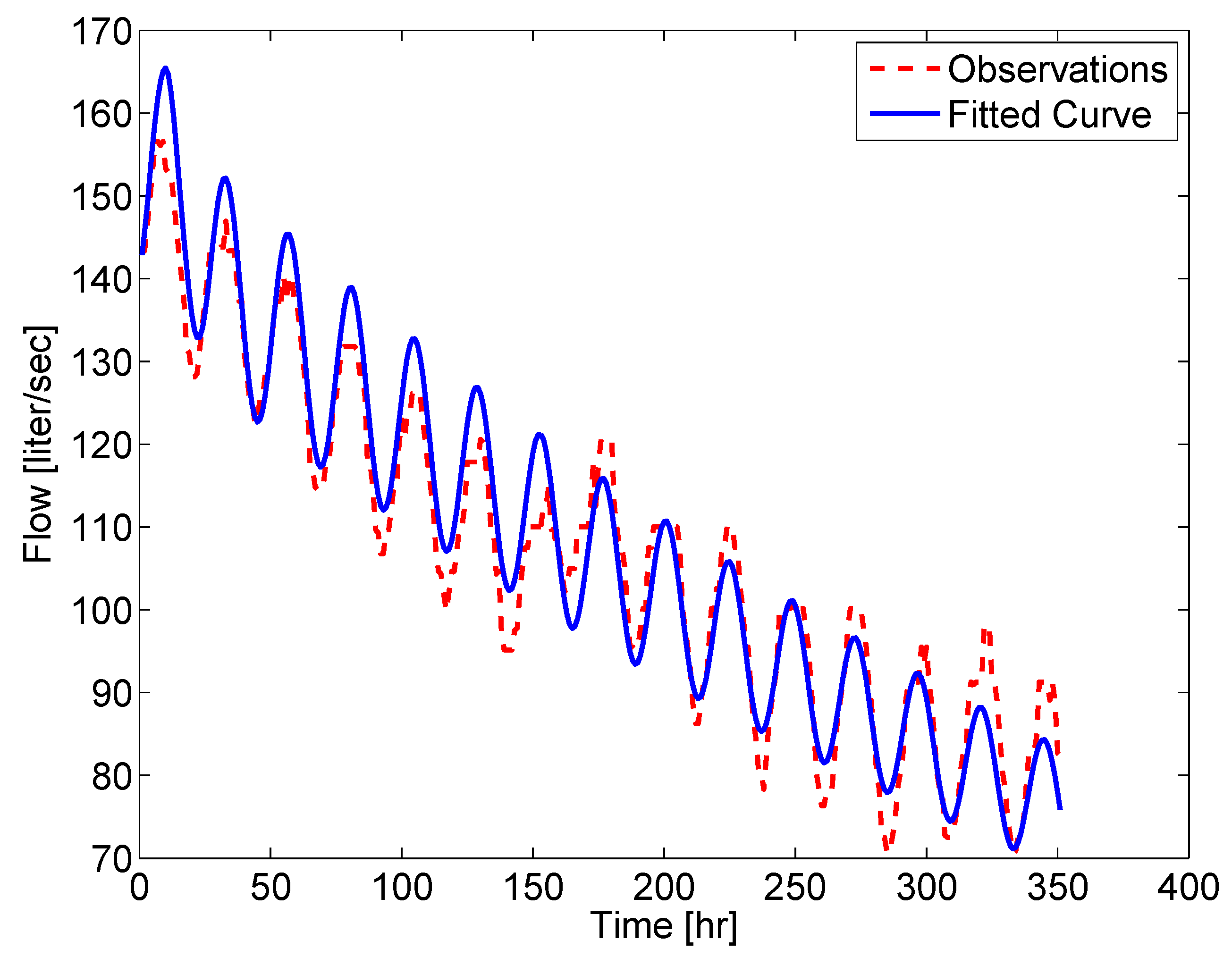
4.1. Application to a Decaying Oscillatory Runoff

Until this point, we have considered a general formula for runoff, called $R\left(t\right)$. We now exemplify our calculations for a prescribed runoff pattern—$R\left(t\right)$ described by Equation (6). In order to numerically investigate the solution of (13) given the function of $R\left(t\right)$ we propose the following approach—(i) we take advantage of the formula of $R\left(t\right)$ to describe it in terms of autonomous ordinary differential equations (see (14) below); then (ii) we compile these ODEs with Equation (13) to obtain the predictive model.

Given the definition (6) of $R\left(t\right)$ with $\omega =2\pi \nu$, we can introduce more convenient variables, $y_1$, $y_2$ and $y_3$ for the autonomous ODE system. First, we choose $y_1=e^{-At}$ and $y_2=e^{-At}sin\left(\omega t\right)$ and compute

$$\begin{array}{cc}\hfill y_1^{\prime }=& -A{y}_1\hfill \\ \hfill y_2^{\prime }=& -A{e}^{-At}sin\left(\omega t\right)+\omega e^{-At}cos\left(\omega t\right),\hfill \end{array}$$

then

$$y_2^{″}=(A^2-{\omega }^2)e^{-At}sin\left(\omega t\right)-2A\omega e^{-At}cos\left(\omega t\right).$$

So

$$y_2^{″}+2A{y}_2^{\prime }=-(A^2+{\omega }^2)e^{-At}sin\left(\omega t\right),$$

or equivalently, $y_2$ as $y_2^{″}+2A{y}_2^{\prime }+(A^2+{\omega }^2)y_2=0$. We convert this ODE to a dynamical system by introducing $y_3=y_2^{\prime }$ and obtaining Equation (14):

$$\begin{array}{cc}\hfill y_1^{\prime }=& -A{y}_1\hfill \\ \hfill y_2^{\prime }=& y_3\hfill \\ \hfill y_3^{\prime }=& -2A{y}_3-(A^2+{\omega }^2)y_2.\hfill \end{array}$$

(14)

From the explicit definitions of $y_1$, $y_2$ and $y_3$, we get the following initial conditions—$y_1\left(0\right)=1$, $y_2\left(0\right)=0$ and $y_3\left(0\right)=\omega$. We select the average value $E{v}_{avg}$ to be the initial value of evaporation, so that the initial value of the corresponding variable $w={\Theta }_R$ is $f\left(E{v}_{avg}\right)$, although this selection is arbitrary. As mentioned, the variables $y_1$, $y_2$ and $y_3$ are convenient choices because we already know the function that describes runoff. In order to rewrite Equation (13) to be in terms of our new variables, we write runoff from Equation (6) and its derivatives as in terms of $y_1$, $y_2$ and $y_3$ as $R=B{y}_1+C{y}_2$, $R^{\prime }=-BA{y}_1+C{y}_3$ and $R^{″}=B{A}^2{y}_1-C(A^2+{\omega }^2)y_2-2AC{y}_3$. Then $a_0$, $a_1$ and $a_2$ from (12) can also be written as functions of $y_1$, $y_2$ and $y_3$, although these formulas are complicated. The fourth equation of the system becomes (Equation (15)):

$${\Theta }_R^{\prime }=a_0(y_1,y_2,y_3)+a_1(y_1,y_2)f^{-1}\left({\Theta }_R\right)+a_2(y_1,y_2,y_3){\Theta }_R,$$

(15)

with $a_0$, $a_1$ and $a_2$ defined according to Equation (12). For example,

$$a_0(y_1,y_2,y_3)=a_0(R(y_1,y_2,y_3),R^{\prime }(y_1,y_3),R^{″}(y_1,y_2,y_3)).$$

The complete system is given by Equation (16):

$$\begin{array}{cc}\hfill y_1^{\prime }=& -A{y}_1\hfill \\ \hfill y_2^{\prime }=& y_3\hfill \\ \hfill y_3^{\prime }=& -2A{y}_3-(A^2+{\omega }^2)y_2.\hfill \\ \hfill {\Theta }_R^{\prime }=& a_0(y_1,y_2,y_3)+a_1(y_1,y_2)f^{-1}\left({\Theta }_R\right)+a_2(y_1,y_2,y_3){\Theta }_R.\hfill \end{array}$$

(16)

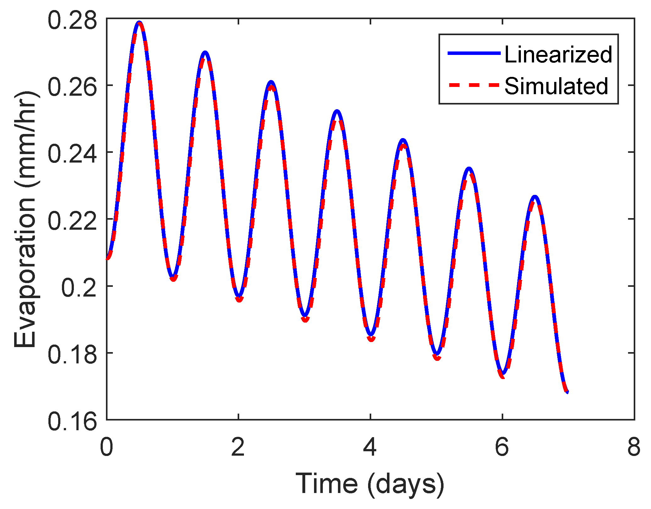
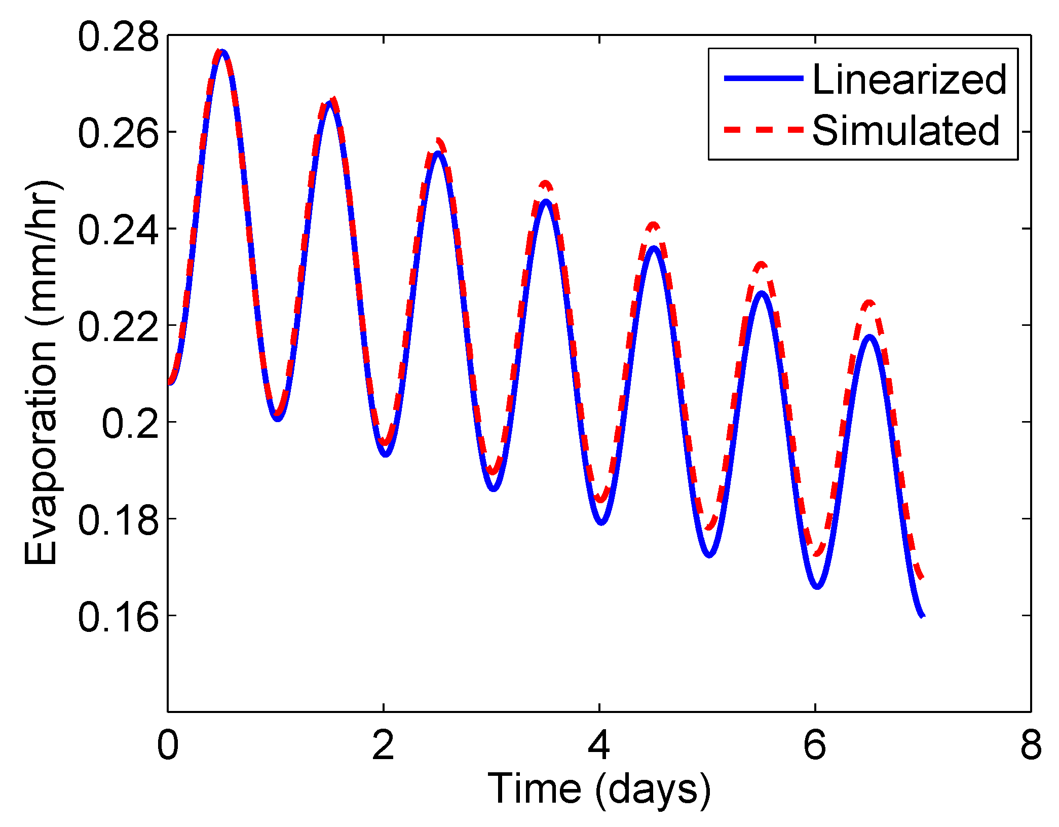
4.2. Finding the Evapotranspiration Solution by Linearizing About the Average Evapotranspiration

In Appendix A, we linearize Equation (13) about the equilibrium point of $Evap=0$, which corresponds to $w={\theta }_N$. Such a linearization yields a close approximation for the solution only insofar as the evapotranspiration forcing is within a small enough neighborhood of the equilibrium point. Because the evaporation is not zero during our simulation and we do not expect it to reach the value zero for a considerable amount of time, we expect a closer approximation if we linearize the system about the average evapotranspiration value. In this section, we find a new solution to the system linearized about the average evapotranspiration value. Certainly the values of evapotranspiration will remain closer to the average value than to zero (the equilibrium value), so we expect a better approximation of the solution to the nonlinear system. We illustrate the linearization process in this section. Because we do not use a prescribed runoff pattern, we will not incorporate the dynamical system as described in Appendix A. Instead we begin with the differential equation given in Equation (13), (repeated here) which does not require a specific runoff pattern or function to describe the dependence of residual soil moisture on evapotranspiration (Equation (17)):

$$\frac{dw}{dt}=a_0(R,R^{\prime },R^{″})+a_1\left(R\right)F\left(w\right)+a_2(R,R^{\prime })w.$$

(17)

We again use the notation $F\left(w\right)=f^{-1}\left(w\right)$ The right hand side of this Equation (17) is a function, call it $g\left(w\right)$. We use a first order Taylor Series approximation for the function as Equation (18):

$$g\left(w\right)\approx g\left(\widehat{w}\right)+g^{\prime }\left(\widehat{w}\right)(w-\widehat{w}),$$

(18)

where $\widehat{w}$ is the value about which we are linearizing ($f\left(E{v}_{Avg}\right)$ in this case). We input the definition of $g\left(w\right)$ so that (Equation (19)):

$$\frac{dw}{dt}\approx a_0+a_{1}F\left(\widehat{w}\right)+a_2\widehat{w}+\left(a_1{F}^{\prime }\left(\widehat{w}\right)+a_2\right)(w-\widehat{w}).$$

(19)

Since $\frac{d(w-\widehat{w})}{dt}=\frac{dw}{dt}$, we could instead write this as Equation (20):

$$\frac{d(w-\widehat{w})}{dt}\approx a_0+a_1{f}^{-1}\left(\widehat{w}\right)+a_2\widehat{w}+(a_1{F}^{\prime }\left(\widehat{w}\right)+a_2)(w-\widehat{w}),$$

(20)

or use the change of variables $w=(w-\widehat{w})$ so that (Equation (21)):

$$\frac{dw}{dt}\approx a_0+a_1{f}^{-1}\left(\widehat{w}\right)+a_2\widehat{w}+(a_1{F}^{\prime }\left(\widehat{w}\right)+a_2)w.$$

(21)

We will solve this differential equation using an integrating factor described herein. Given the differential equation Equation (22):

$$\frac{dw}{dt}+p\left(t\right)w=h\left(t\right),$$

(22)

suppose there is a function $\mu \left(t\right)$ such that $\mu \left(t\right)p\left(t\right)={\mu }^{\prime }\left(t\right)$. Multiplication by the integrating factor, $\mu \left(t\right)$ yields (Equation (23)):

$$\mu \left(t\right)\frac{dw}{dt}+\mu \left(t\right)p\left(t\right)w=\mu \left(t\right)h\left(t\right).$$

(23)

Due to the constraint on $\mu \left(t\right)$, the left hand side can be rewritten as the derivative of a product as Equation (24):

$${\left(\mu \left(t\right)w\right)}^{\prime }=\mu \left(t\right)h\left(t\right),$$

(24)

so that the solution for w is easily found through integration as Equation (25):

$$w=\frac{\int \mu \left(t\right)h\left(t\right)dt+c_1}{\mu \left(t\right)},$$

(25)

where $c_1$ is a constant of integration. Because $\mu \left(t\right)$ is part of the solution, we must also compute it. Since ${\mu }^{\prime }\left(t\right)=\mu \left(t\right)p\left(t\right)$, we can again solve this differential equation using integration to get Equation (26):

$$\mu \left(t\right)=c_{2}exp\left(\int p(t)dt\right).$$

(26)

We apply this solution to Equation (21) by setting $p\left(t\right)=a_1{F}^{\prime }\left(\widehat{w}\right)+a_2$ and $h\left(t\right)=-a_0-a_1{f}^{-1}\left(\widehat{w}\right)-a_2\widehat{w}$.

Using the same runoff pattern described in Section 4.1, the resulting system from linearizing about the average evapotranspiration value is given in Equation (27).

$$\begin{array}{cc}\hfill y_1^{\prime }=& -A{y}_1\hfill \\ \hfill y_2^{\prime }=& y_3\hfill \\ \hfill y_3^{\prime }=& -2A{y}_3-(A^2+{\omega }^2)y_2.\hfill \\ \hfill \frac{dw}{dt}=& h\left(t\right)-p\left(t\right)w.\hfill \end{array}$$

(27)

5. Numerical Example—Doing Hydrology Backwards on a Realistic Catchment

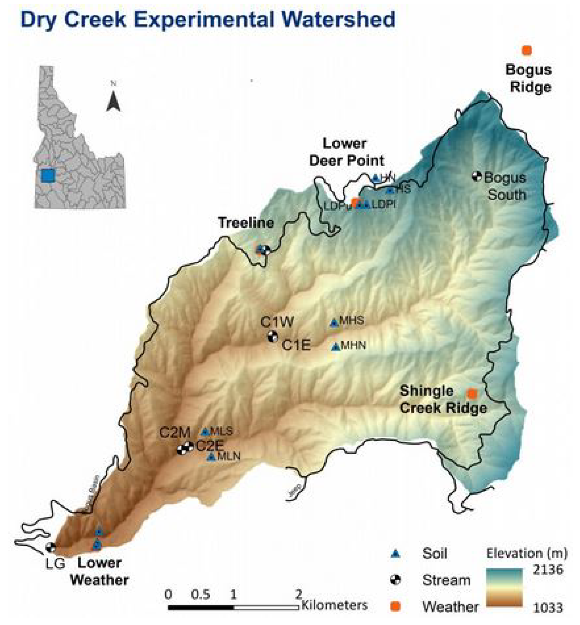
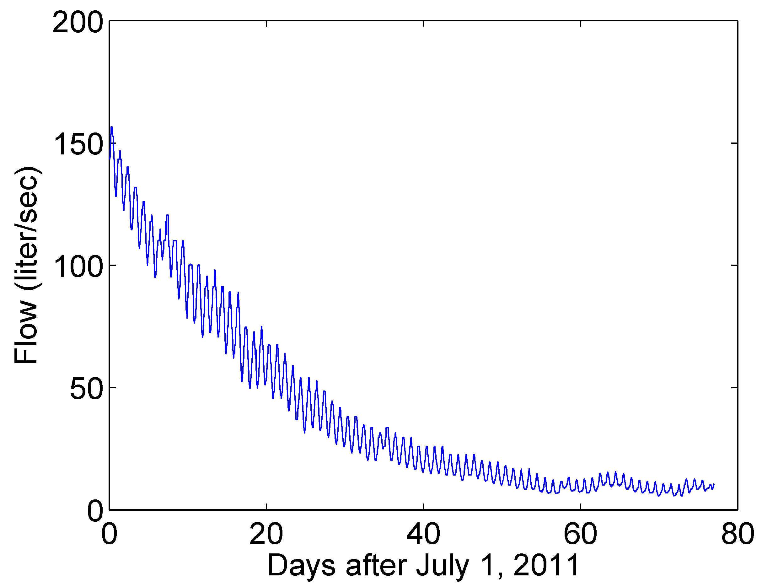
In this section, we apply the results of the previous sections to data from a realistic catchment. Figure 3 provides an overview of the processes described in Section 2, Section 3 and Section 4. We begin with the streamflow at the outlet of the catchment and use it to determine the runoff pattern exiting each hillslope as described in Section 2. Once we know the parameters A, B and C to specify runoff from each hillslope, we use the hillslope subsurface model from Section 3.3 and the results of Section 4 to determine the evapotranspiration forcing that produces the desired runoff pattern at the hillslope scale. Although not presented as a distinct section, computation of fluctuations in the saturated zone is highlighted here because the water table is a feature of many subsurface hillslope models and can be used to compare model results.

5.1. Available Data

The Dry Creek Experimental Watershed is a research laboratory established by Boise State University. The area of the catchment is 28 ${\mathrm{km}}^2$ and it is comprised of 633 hillslopes. The region experiences very little rain, receiving most of its 1000 mm of annual precipitation in the form of snowfall. During the summer, the conditions are dry, the streamflow exhibits the diel-oscillatory behavior described in the literature (e.g., References [13,20,24,25,27,28]).

The site contains seven stream gauging stations and five meteorological stations at different elevations whose locations are shown in Figure 4. Additionally, measurements of soil moisture are taken at eleven locations in the watershed. Stream gauges take hourly measurements of flow in $(\mathrm{L}·{\mathrm{s}}^{-1})$. Streamflow measurements at the outlet of the Dry Creek watershed are used for computation and can be found in Reference [29].

5.2. Determining Hillslope Runoff from Streamflow at The Outlet

The observed streamflow at the outlet of this river network during the summer of any given year exhibits exponential decay with daily oscillations whose amplitude also decays exponentially (see Figure 5 for example).

Streamflow measurements from the lower gauge (at the outlet of the Dry Creek watershed) are taken from July of 2011. Backward hydrology in the network yields the runoff pattern entering each river link. We assume runoff will take the form prescribed by

$$R\left(t\right)=B{e}^{-At}+C{e}^{-At}sin\left(\omega t\right)$$

(as in Equation (6)) and we seek to find appropriate parameter values A, B and C to specify the runoff.

We assume a uniform river network so that the streamflow at the outlet is modeled by the complete solution developed in Reference [19]. The streamflow solution contains the parameters (and combinations of) A, B, C and k ($\nu$ was fixed to maintain the observed period of 24 h).

In order to find best-fit parameters, we use MATLAB’s statistics package [30], whose Nonlinear Regression Model class contains a fitting tool which employs an iterative procedure to estimate model coefficients given initial values. To achieve best results, we apply the fitting tool twice—first after fixing C and k to reasonable values, while A and B are determined using nonlinear regression applied to the uniform streamflow solution. A and B are then fixed to their newly computed values and the code is applied again, this time fitting the parameters C and k, although k is not relevant since it is not found in the function for runoff.

The resulting parameter values are (Equation (28)):

$$\begin{array}{ccc}\hfill A=& 1.89\times {10}^{-3}\hfill & \hfill \left[{\mathrm{hr}}^{-1}\right]\\ \hfill B=& 0.227\hfill & \hfill [\mathrm{liter}·{\sec }^{-1}]\\ \hfill C=& 0.0661\hfill & \hfill [\mathrm{liter}·{\sec }^{-1}],\end{array}$$

(28)

so that the runoff from each hillslope is given by (Equation (29)):

$$R\left(t\right)=0.227e^{-0.00189t}+0.0661e^{-0.00189t}sin(0.0044t).$$

(29)

Following the results of Reference [19], we confirm that these parameters describe runoff which produces a good fit for the streamflow at the outlet by simulating the system in the forward direction using this function to describe runoff from each hillslope. The results can be found in Figure 6.

5.3. Finding the Evapotranspiration Required to Produce Prescribed Runoff Pattern

In this section, we determine the pattern of evaporation that must be applied to each hillslope of the Dry Creek experimental watershed in order to produce the required hillslope runoff. We assume runoff takes the pattern is described by Equation (29) and use parameter values from

Table 3. Parameter values to be used for simulations of the system (8).

Parameter	Value	Units	Physical Meaning
$T_L$	0.1	meter	Depth of top layer of subsurface
$b_L$	0.4	meter	Depth of bottom layer of subsurface
			Includes vadose and saturated zones
$k_2$	$4.1\times {10}^{-3}$	${\min }^{-1}{\mathrm{m}}^{-2/3}$	Rate of movement to link
$k_i$	$2.7\times {10}^{-4}$	${\min }^{-1}$	Rate of movement using preferential flow
$k_{dry}$	$6.7\times {10}^{-3}$	${\min }^{-1}$	Rate of infiltration
$k_3$	$6.9\times {10}^{-8}$	${\min }^{-1}$	Rate of flow exiting subsurface
${\Theta }_N$	0.1	Unitless	Residual soil moisture at night
${\Theta }_D$	0.9	Unitless	Residual soil moisture during day

in the simplified hillslope model under dry conditions (9).

Figure 7 shows the results of simulating Equation (16) along with the solution to the linearized system given in Equation (27). In either of the evapotranspiration patterns from Figure 7, we see oscillations with a period of one day. Because the runoff pattern exiting the system contained an oscillatory function with a period of one day, we expect the forcing terms to have the same period. Moreover, a period of one day is expected for evapotranspiration, since it is dependent upon the daily cycle of temperature.

In addition to oscillations, the value of evapotranspiration is decreasing over time. In this case, we have computed evapotranspiration that forces our hillslope model. This is not necessarily the same as potential evapotranspiration, which depends upon factors like temperature, radiation levels or humidity. Instead we compute actual evapotranspiration, which depends heavily upon the amount of water available in the subsurface. As the hillslope drains, less water is available to be evaporated (or removed by vegetation), so the forcing term decreases over time. Because we linearize about an evapotranspiration value which is likely to occur during our simulation (rather than the equilibrium value of zero, which is unlikely to occur), we expect these results to be close to the true solution, as shown in Figure 7.

Our results indicate that the evapotranspiration pattern at the hillslope scale is qualitatively similar to the observed streamflow. We would like to investigate the accuracy of this concept by examining datasets which contain time-synchronized evapotranspiration and streamflow data at the hillslope scale. We have struggled to find datasets that include evapotranspiration records to the same precision as the streamflow measurements in the same watershed.

6. Conclusions

In this work, we have described methods of doing hydrology backwards in two ways—from the catchment scale to the hillslope scale and from the runoff (output) to the forcing (input) at the hillslope scale. Our methods involve making appropriate assumptions and mathematically inverting corresponding hydrologic models. We first assume constant velocity in the river network and uniformity of hillslopes, which permits us to apply a linear transport model and the analytic solution for streamflow (developed in Reference [19]) to determine the runoff entering each river link from the adjacent hillslope. To employ the analytic streamflow solution, which is appropriate when precipitation is absent, we have focused our efforts on inferring evapotranspiration patterns during dry periods in the catchment.

After finding the runoff from each hillslope, we assumed a simple model to describe water movement through the subsurface. The implications of using the simplified model yielded insights regarding flow through the subsurface and led to a modified subsurface model. With the subsurface model and the runoff output, we developed a system of ODEs that included a variable for residual soil moisture, which is directly related to evaporation. Finally, we again applied the principles behind doing hydrology backwards by solving the system analytically. To do this, we linearized the system about the equilibrium point and simulated the original nonlinear system in MATLAB for comparison. The resulting evapotranspiration solutions exhibit properties that are consistent with expected values. Moreover, we have linked oscillations of the groundwater table with oscillations at the catchment outlet by way of surface runoff.

We conclude that doing hydrology backwards is a viable method for determining the forcing pattern applied to a hydrologic model when output observations are more easily obtained. Because our methodology is mathematical in nature, it requires that we make strong assumptions and invert the corresponding hydrologic models. The strength in this work is that we can now provide a null hypothesis for testing hydrologic models. Our assumptions allow us to provide conjecture about the evapotranspiration cycles in the catchment, so that the assumptions themselves can be validated through experimentation.

References

1. Martina, M.L.V.; Entekhabi, D. Identification of runoff generation spatial distribution using conventional hydrology gauge time series. Water Resour. Res. 2006, 42. [Google Scholar] [CrossRef]
2. Kirchner, J.W. Catchments as simple dynamical systems: Catchment characterization, rainfall-runoff modeling, and doing hydrology backward. Water Resour. Res. 2009, 45. [Google Scholar] [CrossRef] [Green Version]
3. Krier, R.; Matgen, P.; Goergen, K.; Pfister, L.; Hoffmann, L.; Kirchner, J.W.; Uhlenbrook, S.; Savenije, H.H.G. Inferring catchment precipitation by doing hydrology backward: A test in 24 small and mesoscale catchments in Luxembourg. Water Resour. Res. 2012, 48. [Google Scholar] [CrossRef] [Green Version]
4. Brocca, L.; Moramarco, T.; Melone, F.; Wagner, W. A new method for rainfall estimation through soil moisture observations. Geophys. Res. Lett. 2013, 40, 853–858. [Google Scholar] [CrossRef]
5. Kretzschmar, A.; Tych, W.; Chappell, N.A. Reversing hydrology: Estimation of sub-hourly rainfall time-series from streamflow. Environ. Model. Softw. 2014, 60, 290–301. [Google Scholar] [CrossRef]
6. Vrugt, J.A.; Ter Braak, C.J.F.; Clark, M.P.; Hyman, J.M.; Robinson, B.A. Treatment of input uncertainty in hydrologic modeling: Doing hydrology backward with Markov chain Monte Carlo simulation. Water Resour. Res. 2008, 44. [Google Scholar] [CrossRef] [Green Version]
7. Fahle, M.; Dietrich, O. Estimation of evapotranspiration using diurnal groundwater level fluctuations: Comparison of different approaches with groundwater lysimeter data. Water Resour. Res. 2014, 50, 273–286. [Google Scholar] [CrossRef]
8. Habib, E.; Krajewski, W.F.; Kruger, A. Sampling errors of tipping-bucket rain gauge measurements. J. Hydrol. Eng. 2001, 6, 129–166. [Google Scholar] [CrossRef]
9. Walter, I.A.; Allen, R.G.; Elliott, R.; Jensen, M.E.; Itenfisu, D.; Mecham, B.; Howell, T.A.; Snyder, R.; Brown, P.; Echings, S.; et al. ASCE’s standarized reference evapotranspiration equation. In Proceedings of the Watershed Management and Operations Management Conferences 2000, Fort Collins, CO, USA, 20–24 June 2000; pp. 1–11. [Google Scholar]
10. Jin, R.; Li, X.; Liu, S.M. Understanding the Heterogeneity of Soil Moisture and Evapotranspiration Using Multiscale Observations From Satellites, Airborne Sensors, and a Ground-Based Observation Matrix. IEEE Geosci. Remote Sens. Lett. 2017, 14, 2132–2136. [Google Scholar] [CrossRef]
11. Mantilla, R.; Gupta, V.K. A GIS numerical framework to study the process basis of scaling statistics in river networks. IEEE Geosci. Remote Sens. Lett. 2005, 2. [Google Scholar] [CrossRef]
12. Reggiani, P.; Sivapalan, M.; Hassandizadeh, S.M.; Gray, W.G. Coupled equations for mass and momentum balance in a stream network: Theoretical derivation and computational experiments. Proc. R. Soc. A 2001, 457. [Google Scholar] [CrossRef]
13. Wondzell, S.; Gooseff, M.; McGlynn, B. Flow velocity and the hydrologic behavior of streams during baseflow. Geophys. Res. Lett. 2007, 34, L24404. [Google Scholar] [CrossRef]
14. Gupta, V.K.; Waymire, E. Spatial variability and scale invariance in hydrologic regionalization. Scale Depend. Scale Invariance Hydrol. 1998, 88–135. [Google Scholar]
15. Menabde, M.; Sivapalan, M. Linking space-time variability of rainfall and runoff fields on a river network: A dynamic approach. Adv. Water Resour. 2001, 24, 1001–1014. [Google Scholar] [CrossRef]
16. Mantilla, R. Physical Basis of Statistical Scaling in Peak Flows and Stream Flow Hydrographs for Topologic and Spatially Embedded Random Self-Similiar Channel Networks. Ph.D. Thesis, University of Colorado at Boulder, Boulder, CO, USA, 2007. [Google Scholar]
17. Krajewski, W.F.; Ceynar, D.; Demir, I.; Goska, R.; Kruger, A.; Langel, C.; Mantilla, R.; Niemeier, J.; Quintero, F.; Seo, B.C.; et al. Real-Time Flood Forecasting and Information System for the State of Iowa. Bull. Am. Meteorol. Soc. 2017, 98, 539–554. [Google Scholar] [CrossRef]
18. Ayalew, T.B.; Krajewski, W.F.; Mantilla, R. Connecting the power-law scaling structure of peak-discharges to spatially variable rainfall and catchment physical properties. Adv. Water Resour. 2014, 71, 32–43. [Google Scholar] [CrossRef]
19. Fonley, M.; Mantilla, R.; Small, S.; Curtu, R. On the propagation of diel signals in river networks using analytic solutions of flow equations. Hydrol. Earth Syst. Sci. 2016, 20, 2899–2912. [Google Scholar] [CrossRef] [Green Version]
20. Burt, T.P. Diurnal variations in stream discharge and throughflow during a period of low flow. J. Hydrol. 1979, 41, 291–301. [Google Scholar] [CrossRef]
21. Duffy, C.J. A two-state integral-balance model for soil moisture and groundwater dynamics in complex terrain. Water Resour. Res. 1996, 32, 2421–2434. [Google Scholar] [CrossRef]
22. Qu, Y.; Duffy, C.J. A semidiscrete finite volume formulation for multiprocess watershed simulation. Water Resour. Res. 2007, 43. [Google Scholar] [CrossRef]
23. Curtu, R.; Mantilla, R.; Fonley, M.; Cunha, L.K.; Small, S.; Jay, L.; Krajewski, W.F. An integral-balance nonlinear model to simulate changes in soil moisture, groundwater and surface runoff dynamics at the hillslope scale. Adv. Water Resour. 2014, 71, 125–139. [Google Scholar] [CrossRef]
24. Bond, B.; Jones, J.; Moore, G.; Phillips, N.; Post, D.; McDonnell, J. The zone of vegetation influence on baseflow revealed by diel patterns of streamflow and vegetation water use in a headwater basin. Hydrol. Process. 2002, 16, 1671–1677. [Google Scholar] [CrossRef]
25. Graham, C.; Barnard, H.; Kavanagh, K.; McNamara, J. Catchment scale controls the temporal connection of transpiration and diel fluctuations in streamflow. Hydrol. Process. 2013, 27, 2541–2556. [Google Scholar] [CrossRef]
26. Ayalew, T.B.; Krajewski, W.F.; Mantilla, R. Exploring the effect of reservoir storage on peak discharge frequency. J. Hydrol. Eng. 2013, 18, 1697–1708. [Google Scholar] [CrossRef]
27. Gribovszki, Z.; Kalicz, P.; Szilágyi, J.; Kucsara, M. Riparian zone evapotranspiration estimation from diurnal groundwater level fluctuations. J. Hydrol. 2008, 349, 6–17. [Google Scholar] [CrossRef]
28. Wondzell, S.M.; Gooseff, M.N.; McGlynn, B.L. An analysis of alternative conceptual models relating hyporheic exchange flow to diel fluctuations in discharge during baseflow recession. Hydrol. Process. 2010, 24, 686–694. [Google Scholar] [CrossRef]
29. Dry Creek Experimental Watershed, Lower Gauge Streamflow Data; Boise State University: Boise, ID, USA, 2015.
30. MATLAB and Optimization Toolbox Release; The MathWorks, Inc.: Natick, MA, USA, 2012.
Figure 1. Sample subsurface pattern given by Equation (6) using A = 0 . 003 ( 1 / h ), B = 0 . 08 ( L · s 1 ), C = 0 . 008 ( L · s 1 ) and ν = 1 24 ( h 1 ).
Hydrology 06 00085 g001
Figure 2. The soil model is described by Equation (8).
Hydrology 06 00085 g002
Figure 3. An overview of the processes described in Section 2, Section 3 and Section 4.
Hydrology 06 00085 g003
Figure 4. The Dry Creek Experimental Watershed in Idaho.
Hydrology 06 00085 g004
Figure 5. Observed streamflow in Dry Creek Experimental Watershed (Lower Gauge) in 2011.
Hydrology 06 00085 g005
Figure 6. Observed streamflow in Dry Creek Experimental Watershed (location Lower Gauge). The data shown is from 1–15 July in 2011.
Hydrology 06 00085 g006
Figure 7. The evaporation pattern obtained from solving system (27) which has been linearized about the average evapotranspiration value and from simulating the nonlinear system in MATLAB.
Hydrology 06 00085 g007