Article

Pollution Source Identification for River Chemical Spills by Modular-Bayesian Approach: A Retrospective Study on the ‘Landmark’ Spill Incident in China

1
Shenzhen Municipal Engineering Lab of Environmental IoT Technologies, School of Environmental Science and Engineering, Southern University of Science and Technology, Shenzhen 518055, China
2
Huayue Institute of Ecological Environment Engineering, Chongqing 401122, China
3
School of the Environment, Nanjing University, Nanjing 210093, China
4
School of Environment, Harbin Institute of Technology, Harbin 150090, China
*
Author to whom correspondence should be addressed.
Hydrology 2019, 6(3), 74; https://doi.org/10.3390/hydrology6030074
Submission received: 20 March 2019 / Revised: 18 August 2019 / Accepted: 19 August 2019 / Published: 20 August 2019

Abstract

:
It is important to identify source information after a river chemical spill incident occurs. Among various source inversion approaches, a Bayesian-based framework is able to directly characterize inverse uncertainty using a probability distribution and has recently become of interest. However, the literature has not reported its application to actual spill incidents, and many aspects in practical use have not yet been clearly illustrated, e.g., feasibility for large scale pollution incidents, algorithm parameters, and likelihood functions. This work deduced a complete modular-Bayesian approach for river chemical spills, which combined variance assumptions on a pollutant concentration time series with Adaptive-Metropolis sampling. A retrospective case study was conducted based on the ‘landmark’ spill incident in China, the Songhua River nitrobenzene spill of 2005. The results show that release mass, place, and moment were identified with biases of −26.9%, −7.9%, and 16.9%, respectively. Inverse uncertainty statistics were also quantified for each source parameter. Performance, uncertainty sources, and future work are discussed. This study provides an important real-life case to demonstrate the usefulness of the modular-Bayesian approach in practice and provides valuable references for the setting of parameters for the sampling algorithm and variance assumptions.

1. Introduction

Intentional or unintentional chemical spills continue to occur not only in developing countries but also in developed countries [1]. In China, there has been a notable increase in the occurrence of environmental accidents in the past decade as a consequence of the increasing activities associated with economic growth [2,3]. As reported by Yao et al. and Li and An [3,4], there have been, on average, approximately 60 surface water pollution accidents each year since 2011. Many soluble pollutants are invisible or cannot be detected on-line when released into rivers and streams. It is very common that only if the effects of pollution are visible, e.g., dead fish floating or dangerous colors shown in a river, that the hazard or spill incident is reported, and the emergency response started. Therefore, quickly identifying the source information for unreported or clandestine incidents would provide scientific support for making mitigation and adaptation strategies in emergency management.
Given known concentrations monitored downstream, the problem of identifying the source characteristics (location, release history, and loading) can be categorized as a “time inversion” problem. This problem has been well established as a subset of “inverse problems” [5]. In the mathematics and engineering fields, it is popularly known as the “inverse source problem” (ISP) [6,7]. Many methods have been developed in the literature for ISP, such as regularization methods [8,9], simulation-optimization methods [9], and Bayesian inference methods [8].
Recently, surface water pollution source identification has received increased attention, and several approaches have been reported. For example, Chen et al. [10] presented the correlation coefficients optimization method. Cheng and Jia [11] developed the backward location probability density function method. Boano et al. [12] successfully applied a geostatistical approach. Wei et al. [13] reported the use of a Bayesian approach. Among them, Bayesian approaches have a number of distinct advantages and have been used in several areas, e.g., reservoir operation [14], water quality model parameters estimation [15], and rainfall-runoff modeling [16]. This approach utilizes probabilistic prior information and observes data to update and provide a posterior probability distribution of the corresponding source parameters and quantify inverse uncertainty, determining the uncertainties of the model inputs due to the uncertainties of given responses [17,18].
Zhu [19] first investigated the Bayesian application in surface water pollution source identification. This early study is based on simple hypothetical cases without reference to specific case studies, and traditional Markov chain Monte Carlo (MCMC) was used. Wang and Harrison [20] used Bayesian and MCMC methods to identify the contaminant profiles in hypothetical water distribution systems. Wei et al. [13] induced source parameter uncertainty analysis before running the Bayesian inference process and adopting Delayed Rejection and Adaptive Metropolis MCMC for sampling posteriors.
However, knowledge gaps still hinder the use of a modular-Bayesian approach in practice. Firstly, the formulation of the modular-Bayesian framework for the ISP of surface water pollution has not been reported in the literature. Technically, it also lacks investigation on how the source inversion performs when using different likelihood functions, the key component of Bayesian inference, based on different error assumptions in monitoring data. Details of parameter setting in Adaptive-Metropolis sampling algorithms [16] for this ISP problem have never been reported. Furthermore, using Bayesian source inversion on real river chemical spill incidents has rarely been investigated because of the challenge of collecting pollution data. Actual pollutant concentration data are not readily available in some cases. Only a few research groups are able to take part in the field work of emergency disposal. Additionally, in many cases, monitoring has one chance to be completed since when incidents are reported and responded to, the pollutant plume has spread into lakes, reservoirs, and coastal areas or run into the mainstream.
Therefore, this study focuses on the Bayesian reasoning application in a historical nitrobenzene spill incident that occurred in the Songhua River, China, in 2005. It is the most severe spill incident in the 21st century in China [21]. Firstly, we present the deduction and establishment of the modular-Bayesian framework for chemical spill oriented ISP. The scenario of emergency monitoring and source identification is reconstructed according to reality. After parameterizing the water quality model and Adaptive Metropolis (AM) sampling algorithm, the modular-Bayesian inference process is calculated. Two types of likelihood functions are used and compared. The results are discussed based on our knowledge of the incidents. Future works are then discussed from the watershed management point of view.

2. Modular-Bayesian Approach for Pollution Source Identification

Bayesian estimation provides a formal mechanism for combining prior information based on historical data or expert knowledge and data collected by observation. In this section, we will deduce the modular-Bayesian framework for ISP problems with regard to river chemical spill incidents.

2.1. General Statement of ISP Problems

For a typical ISP problem, n samples are collected with the data C, which is also relative to the forward modeling operator g. This operator g maps models into a data space. Taking the river chemical spill for instance (Figure 1), C stands for a group of in-stream pollutant concentrations, and g stands for the in-stream water quality model, i.e., the pollutant transport model.
In practice, the forward operator is always an approximation. Therefore, there is a systematic error associated with the use of g in modeling. Let us represent it by an n-dimensional vector emodel. There is also an n-dimensional vector of random observation errors, denoted as eobs. The connection between the model and observed data can be represented as:
C = g(s;m) + eobs + emodel,
where s represents the unknown source parameters, and m denotes the known model parameters. The goal is to estimate s [or a function of s, L(s)] given a vector of C [22]. It should be noted that s could sometimes be the boundary conditions or initial condition in the forward model. For river pollution sources, s normally covers release time ts, location xs, and total load Ms, as well as the release history L(s).

2.2. Model-Based Bayesian Inferences

The Bayes theorem provides a formal framework for combining the prior information based on historical data and expert knowledge with observational data. In the context of the ISP, Bayes theorem can be stated as follows:
p ( s | C , I ) = p ( s | I ) l ( C | s , I ) p ( C | I ) ,
p ( C | I ) = a l l s p ( s ) l ( C | I , s ) d s ,
where p(s|C,I) is the posterior distribution of source parameters given C and I, p(s|I) is the prior, l(C|s,I) is the likelihood, p(C|I) is the evidence, s is the source term, C is the observation data at a given location x and time t, and I is the information (e.g., that is used to determine the prior distribution of s). The probability can be substituted by the probability distribution function p.
The procedure of model-based Bayesian inference can be summarized into four steps [23]: model building, calculation of the posterior distribution, analysis of the posterior distribution, and inference.

2.2.1. Step 1: Model Building

(1) Bayesian formulation for ISP
Let Ci and Ri denote the observed and modeled concentrations, respectively, at location xi and time ti, where i = 1,…, n; and (xi, ti) is the sampling pair. It can be assumed that any discrepancy between Ci and Ri arises from two sources: the measurement errors e i o b s and mechanism model errors e i m o d e l . Let us also assume that the errors have a standard normal distribution, N ( 0 , σ o b s , i ) and N ( 0 , σ m o d e l , i ) , respectively.
For e i o b s , Ctrue,i is the unknown true value of the concentration at the sampling point at a given time, i.e., (xi, ti). Therefore, Ci = Ctrue,i + e i o b s . Similarly, for the model, Ri = Ctrue,i + e i m o d e l . The difference between measured and modeled values can be written as CiRi = e i o b s e i m o d e l , which bridges a connection between the source and measurement data.
In practice, however, there will be n different normal distributions of measurement errors and another n of model errors. Each sampling and analysis process of chemical concentration will also induce its own e i o b s . For simplicity, it is safe to assume an independent distribution of all the ns of σ o b s , i and σ m o d e l , i . The joint distributions are as follows:
C i R i = N ( 0 , σ o b s , i 2 + σ m o d e l , i 2 ) ,
R i = N ( C i , σ o b s , i 2 + σ m o d e l , i 2 ) ,
where we take Ci as a constant, while Ri is a stochastic variable derived from the stochastic parameter s.
The conditional probability under the condition of knowing the real value Ctrue to get the observed values of Ci can be written as the formula below:
p ( C | C t r u e , I ) = i { ( 2 π σ o b s , i 2 ) 1 / 2 e x p [ ( C i C t r u e , i ) 2 2 σ o b s , i 2 ] } e x p [ i ( C i C t r u e , i ) 2 2 σ o b s , i 2 ] .
It is the joint probability distribution function (PDF) of n numbers of samples. If we assume all the measurement error to be independently and identically distributed (IID), then all the n of σ o b s , i are equal to σ o b s and Equation (6) becomes:
p ( C | C t r u e , I ) e x p [ 1 2 i ( C i C t r u e , i ) 2 σ o b s 2 ] .
Equation (7) represents the probability that the observed concentrations are measured as C when the true values are actually Ctrue and are proportionate to the right term. Furthermore, we obtain Equation (8)
p ( C t r u e | s , I ) = i { ( 2 π σ m o d e l , i 2 ) 1 / 2 e x p [ ( R i C t r u e , i ) 2 2 σ o b s , i 2 ] } e x p [ i ( R i C t r u e , i ) 2 2 σ m o d e l , i 2 ] ,
where σ is the known constant, which refers to p ( C t r u e | s , I ) . The model error is then given by Equation (9) with the same IID assumption.
p ( C t r u e | s , I ) e x p [ 1 2 i ( C t r u e , i R i ( s ) ) 2 σ m o d e l 2 ] .
It states the probability that the true data (e.g., pollutant concentration) are predicted by the forward model, e.g., the pollutant transport model here, when the source parameters are s.
The likelihood is then obtained by marginalizing the joint PDF of C and Ctrue with respect to Ctrue:
p ( C | s , I ) = i { ( 2 π σ o b s , i 2 ) 1 / 2 e x p [ ( C i C t r u e , i ) 2 2 σ o b s , i 2 ( R i C t r u e , i ) 2 2 σ m o d e l , i 2 ] } d C t r u e .
Evaluating the integral of Equation (10) yields the likelihood:
p ( C | s , I ) e x p [ i ( C i R i ) 2 2 ( σ o b s , i 2 + σ m o d e l , i 2 ) ] .
Further, if we take σ a l l 2 = σ o b s 2 + σ m o d e l 2 , since σobs and σmodel are interchangeable and cannot be distinguished from the data, therefore:
p ( C | s ) = ( 2 π σ a l l 2 ) n / 2 i e x p [ ( C i R i ) 2 2 σ a l l 2 ] .
If C and σ a l l are known, calculating R i ( s ) for various s yields p ( C | s , I ) . The problem is transferred to the estimate σ a l l .
It should be noted that the abovementioned error terms e i o b s and e i m o d e l are assumed to be homoscedastic and uncorrelated. One can also assume that the errors are different, such as heteroscedastic and uncorrelated and heteroscedastic and correlated. Therefore, depending upon the type of errors, there will be different likelihood functions. Further details on such likelihood function can be seen in Bates and Campbell [24].
The variance of the heteroscedastic uncorrelated error term can be stabilized using the class of transformation, Box-Cox transformation, of the original monitoring data as in Equation (13), especially when a large data size is available [25,26]. It has demonstrated the feasibility of this transformation on hydrological datasets and is widely used [26,27]. Other new power distribution approaches like the recently proposed log-sinh transformation [28] are not tested in this work.
X t = { ( C i + λ 2 ) λ 1 1 λ 1 , λ 1 0 log ( C i + λ 2 ) , λ 1 = 0 .
Here, λ1 can be estimated from the mean residual of Ci. If the variance of the binned mean residuals increase linearly with the mean, then one can set λ1 = 0.5; if the variance increases quadratically with the mean, then one can set λ1 = 0 [24]. Worth noticing, the Box-Cox transformation’s primary motivation is to restore a greater degree of normality in the transformed data. It is not, strictly speaking, a variance-stabilizing transformation, although that may be a by-product of the transformation process.
The likelihood function based on the assumption of a heteroscedastic uncorrelated error term is given by:
p ( C i | s ) = ( 2 π σ 2 ) n / 2 n e x p { [ log ( C i + λ 2 C m o d e l , i + λ 2 ) ] 2 2 σ a l l 2 } ( C i + λ 2 ) 1 ,   λ 1   =   0 ,
where σall is the variance of Ci.
(2) Assignment of the prior probability
The requirement of using the Bayes approach to conduct statistical inferences is assigning a prior probability to the parameters. Several alternatives are available to the assignment of a prior probability [29]: (a) the objective method or so called empirical Bayes method, which is based on historical data or knowledge; (b) the subjective probability method, which assigns the prior PDF based on personal understanding; (c) the principle of indifference, which assigns equal probabilities to all possibilities, i.e., uniform PDF; and (d) the conjugate prior, which makes prior PDF and posterior PDF the same distribution type from a purely mathematical point of view. Approaches can also be classified as noninformative, highly informative, and moderately informative ways [30].
In hydrology studies, the empirical Bayes method is usually used, i.e., distribution from historical records, and the prior is set as a Gamma distribution, normal distribution, uniform distribution, etc. [30,31]. However, information for assigning the prior PDF of source parameters is usually quite limited in many real-life cases. Therefore, a non-informatively uniform distribution seems to be the first choice here. If potential environmental risk sources, such as the chemical industry and livestock farms, are located along the objective river reaches, we can give priority to the possibility that the pollution source was released in those sections and set an integrated PDF. The prior probability of a uniform distribution can be given as follows:
p ( s | I )   =   constant ,   s R .
(3) The posterior probability density function
The homoscedastic posterior probability density function can be presented as follows:
p ( s | C , I ) p ( s | I ) p ( C | s , I ) I ( s R ) e x p [ 1 2 i ( C i R i ( s ) ) 2   σ o b s 2 + σ m o d e l 2 ] ,
where I denotes the indicator function.

2.2.2. Step 2: Calculation of the Posterior Distribution—MCMC Sampling

The posterior distribution is always not conjugated (with regard to posterior), and the approximation is intractable, or the full conditionals do not look like any known distributions. Therefore, techniques based on drawing dependent samples from the posterior distribution are developed. A broad class of techniques, collectively referred to as Markov chain Monte Carlo (MCMC), has been reported since the mid-twentieth century. The Metropolis–Hastings (MH) algorithm [32,33] and Gibbs sampling [34] are two of the most important techniques used in MCMC [35].
Many variants and extensions of these algorithms have been proposed in the literature to date. Although they are based on the same principles of the original algorithms, most of them are more advanced and complicated than the original ones and usually focus on specific problems. In this study, the Adaptive Metropolis algorithm is adopted for this ISP-oriented Bayesian inference framework.
In the conventional MH algorithm, the posterior distribution of the model parameter θ = (θ1θd), where d is the number of iterations, is sampled as Marshall et al. [16]. One variation of the conventional MH algorithm is the AM algorithm [36], which was used in this study. The AM algorithm is characterized by a proposal distribution based on the estimated posterior covariance matrix of the parameter; the posterior covariance matrix is calculated at each iteration based on past iterations. Thus, the proposal distribution is updated using the knowledge learned so far about the posterior distribution.
Many approaches have been developed to diagnose the convergence of the Markov chain [37]. The convergence diagnostics developed by Gelman and Rubin and Raftery and Lewis [38,39] are currently the most popular among the statistical community. We use the Gelman–Rubin potential scale reduction factor (R) to diagnose the convergence of the algorithm in this work. See Gelman and Rubin [38] for more details.

2.2.3. Step 3: Analysis of the Posterior Distribution

There are two ways to analyze the posterior distribution available: (1) statistical measurement of the posterior samples using the mean, square deviation, median values, fractal quantile, skewness, and other descriptive statistics; and (2) calculating the marginal distribution of source parameters by the numerical integration. For example, xs can be calculated by Equation (17) [18]. In this work, we adopt the first option for easily understanding by decision makers.
P ( x s | C , I ) = a l l M s   a l l t s P ( x s , t s , M s | C , I ) d t s d M s .

2.2.4. Step 4: Inference

In this final step, an inference on source information was made based on the above results. It adopts median values of xs and Bayesian intervals as the final inference. To be sure, physical investigations in the field have to be conducted in practice to confirm the real source information.

2.3. Solute Transport in Rivers (Forward Model)

The following coupled hydrodynamics-water quality system is able to describe the soluble pollutant transport behavior in rivers and streams:
· u = 0 ,
u t + u u = p ρ + v 2 u ,
c t + u c = ( D c ) K c + S ,
where u is the velocity vector of the fluid parcel, ρ is the fluid density, ν is the kinematic viscosity, p is the pressure, c is the pollutant concentration, D is the diffusion coefficient, K is the pollutant degradation coefficient, and S is the source term of the pollutant. Equation (19) is the Navier–Stokes equations of incompressible fluid flow, and Equation (20) is an advection-diffusion-reaction (ADR) equation based on first-order reaction kinetics.
It is normal that hydrodynamic processes and water quality processes are considered independently for inland water. The shallow water equation is a common simplification of hydrodynamic processes. For the steady-state, the ADR equation has an analytic solution, which is very useful for first responders. For single sources with impulse discharge, depicted by the delta function s = M 0 δ ( x x s ) δ ( t t s ) , the theoretical concentration at the point (x, t) can be calculated by the following formula [10]:
C ( x , t ) = M s A 4 π D x ( t t s ) e x p [ ( x x s Ut + U t s ) 2 4 D x ( t t s ) ] e x p [ K ( t t s ) ] ,
where A is the area of the river’s cross section (m2), Dx is the average longitudinal dispersion coefficient (m2/min), U is the average river velocity (m/min), K is the decaying coefficient (min−1), t is the monitored time (min), and x denotes the location of the monitoring site.

3. Case Study on the Songhua River Nitrobenzene Spill Incident

3.1. Description of the Songhua River Nitrobenzene spill

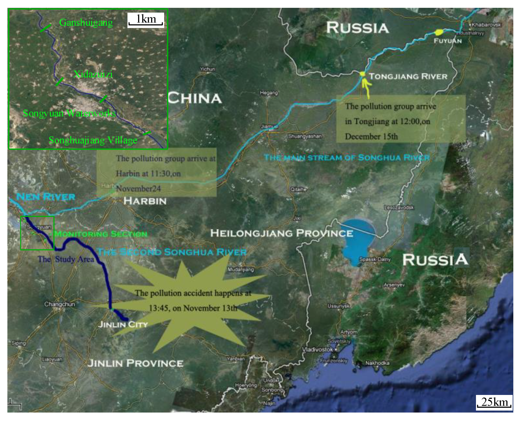
The Songhua River (Figure 2), located in Northeast China, is the third largest river basin in China. It covers a 5,568,000 km2 area and runs through four provinces where 62 million residents live. What is commonly referred to as the Songhua River includes the Second Songhua River in the Jilin Province and the main stream in the Heilongjiang Province. Its headstream has two sources: the Nen River (north source) and the Second Songhua River (south source). The two run confluent at Sanchahe, developing the main stream of the Songhua River (939 km). At Tongjiang City, the Songhua River flows into the Heilongjiang River (Amur River), the Sino-Russian boundary river. Finally, it runs into the Okhotsk Sea [40,41].
The Songhua River nitrobenzene spill incident, due to the explosion that occurred at a petrochemical plant of the Jilin Petrochemical Co in Jilin City, Jilin Province, in 2005, is a ‘landmark’ spill incident in China. An estimated 100 tons of mixtures of benzene, aniline, and nitrobenzene with firefighting water spilled into the Songhua River [21,42]. The whole pollutant plume moved across two provinces, four cities, and 26 counties in 43 days. As the pollutant plume flowed downstream, the spill lead to the suspension of Harbin’s (the capital of the Heilongjiang Province with a population of 4 million) water supply and a Russian lawsuit against China. After this ‘landmark’ spill incident, the Chinese government put a lot of effort into developing emergency response technologies for pollution incidents. This case study is conducted based on this typical historical event to illustrate the usefulness and merits of the modular-Bayesian approach in practice.

3.2. Reconstructed Source Identification Scenario

The source identification scenario was reconstructed as follows. The Second Songhua River in the Jilin Province (dark blue river reach in Figure 2) was selected as the objective study area, which is more reasonable for emergency pollution source inversion than in the mainstream. Compared with the mainstream of the Songhua River in the Heilongjiang Province, the Second Songhua River has fewer tributaries and is closer to the release location.
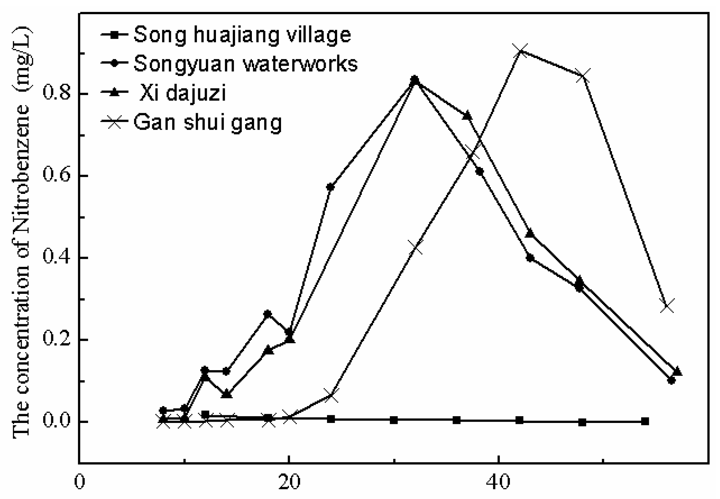
We assume the national monitoring section at Ganshuigang (the green section closest to the mainstream in Figure 2) first detected and reported the nitrobenzene in the water. Then, emergency monitoring was planned, and monitoring sections were set in the upstream of the Ganshuigang section. In total, four nationally controlled monitoring sections were set for sampling: Songhuajiang Village, Songyuan Waterworks, Xidazuizi, and Ganshuigang, which are 155, 276, 281, and 336 km downstream of the release point, respectively. According to the real monitoring process during the incident and the available concentration data, the monitoring period ranged from 6 p.m., 18 November 2005 to 7 p.m., 19 November 2005 (25 h), with a frequency of 2 to 6 h. The origin of the space-time coordinate axis was defined as the Baiqi monitoring section (75 km downstream the release location) and 0 a.m., 16 November 2005 (convenient for time conversion). Figure 3 presents the nitrobenzene breaking through curves obtained during the monitoring period.
It should be noted that emergency monitoring for source inversion would have been completed in a short period. However, we have no choice and have to use the available monitoring data collected at the time, which are restricted to the real sampling conditions and response. For a retrospective study, this is acceptable. Compared with the 43 days of pollutant plume transportation on the river, one day of upstream monitoring is also acceptable for emergency response.

3.3. Parameters of Forward Model and Bayesian Inference Process

We assumed the pollutant load Ms equaled 92 tons (nitrobenzene), as was reported and estimated. Since it is rational to use a simple water quality model for first responders, a one-dimensional pollutant transport model was used, as depicted in Equation (21). The average flow velocity U is the mean value of historical hydrological observations in the same period. The longitudinal diffusion coefficient Dx can be estimated by the Fisher formula as follows [43]:
D x = 0.011 u ¯ 2 × B 2 d × u ± 50 % ,
where u ¯ is the average flow velocity, B is the width of the river, d is the depth of the river, u is the shear velocity of the river equal to g × d × s , g is the gravitational acceleration, and s is the slope of the river.
Due to 50% of the relative errors induced by using the Fisher formula, Dx was revised and rounded after comparison with the study [40]. The cross-section area of the given reach is estimated by average streamflow and flow speed. Nitrobenzene decay coefficients were obtained from the literature. Table 1 lists the values of the source and model parameters. We also assumed that those parameters can be easily and quickly obtained from field work and literature inquiry.
Worth noticing, two- or three-dimensional models are more popular nowadays for forward modelling [45,46,47]. However, due to the challenges of calibration on large scale (about 100 km) rivers and association with physical search of pollution sources in practices, the one-dimensional model was tested here for a real-life case study. Other options are using surrogate models such as neural networks like in [48,49].
The prior PDF and AM algorithm parameters were set as in Table 2. The prior distribution of pollution discharge parameters were set as a uniform distribution: Ms~U (20 tons, 200 tons), xs = U(−200 km, 5 km), and ts = U(−72 h,−24 h), where the boundaries of the parameter interval were empirically assumed and rounded. The prior PDF of source vector s is generated by the joint distribution of Ms, xs, and ts. It is also assumed that errors were not related both for homoscedastic (Run 1) and heteroscedastic (Run 2) samples, and sampling was conducted 100,000 times. For Run 1, the incipient 20,000 sampling times were discarded for final statistical calculation. For Run 2, the latter 80,000 sampling times were used in the final statistical calculation. If the acceptance rates were outside the range of 25–75% (see [16]), manually tuning the proposal scaling factor, sd, would be adopted to adjust the proposal density (see [16]). Moreover, here, the AM algorithm calculated the log transformation of the likelihood function. Other parameters can be seen in Table 2.

3.4. Inversion Results

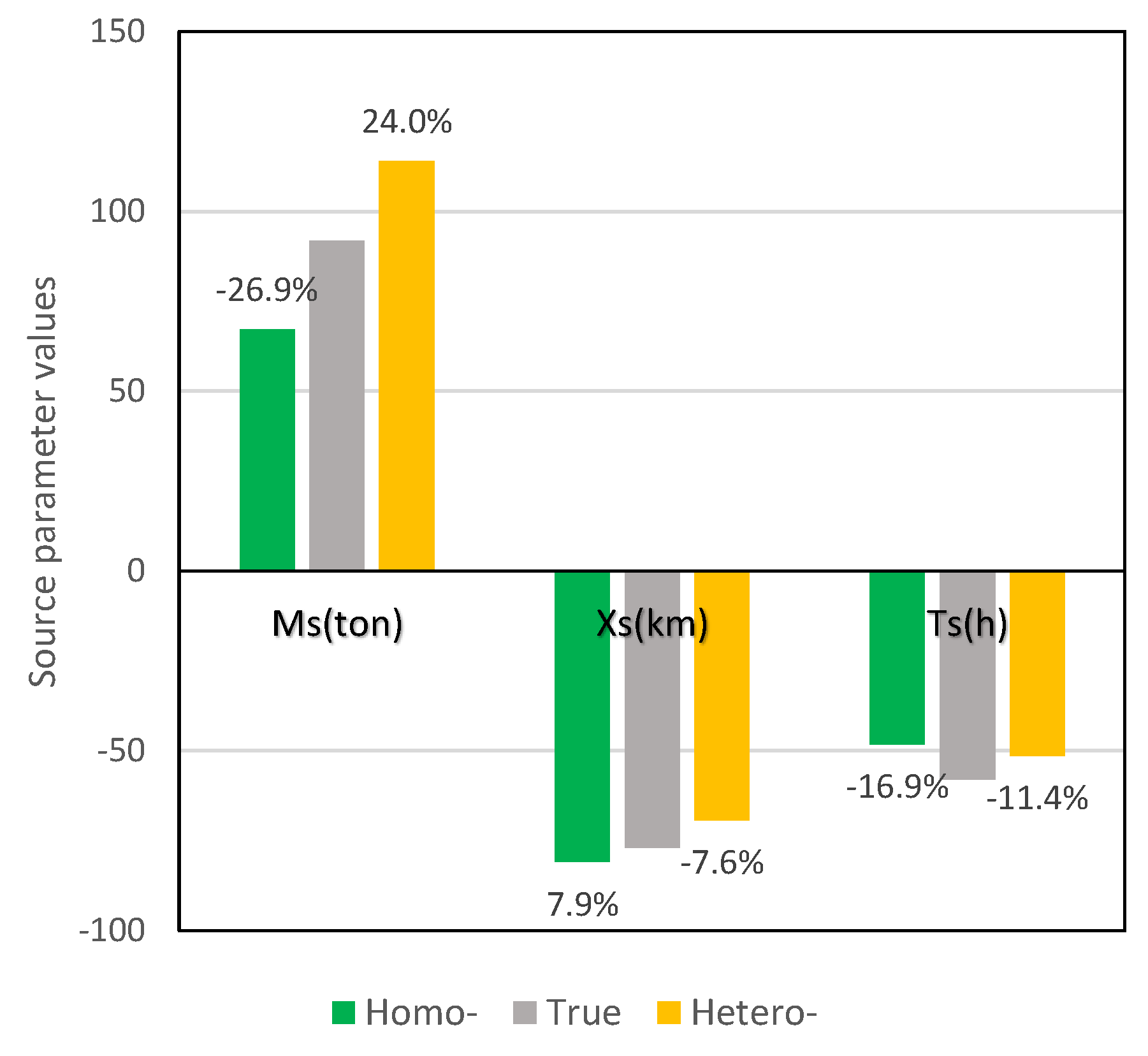
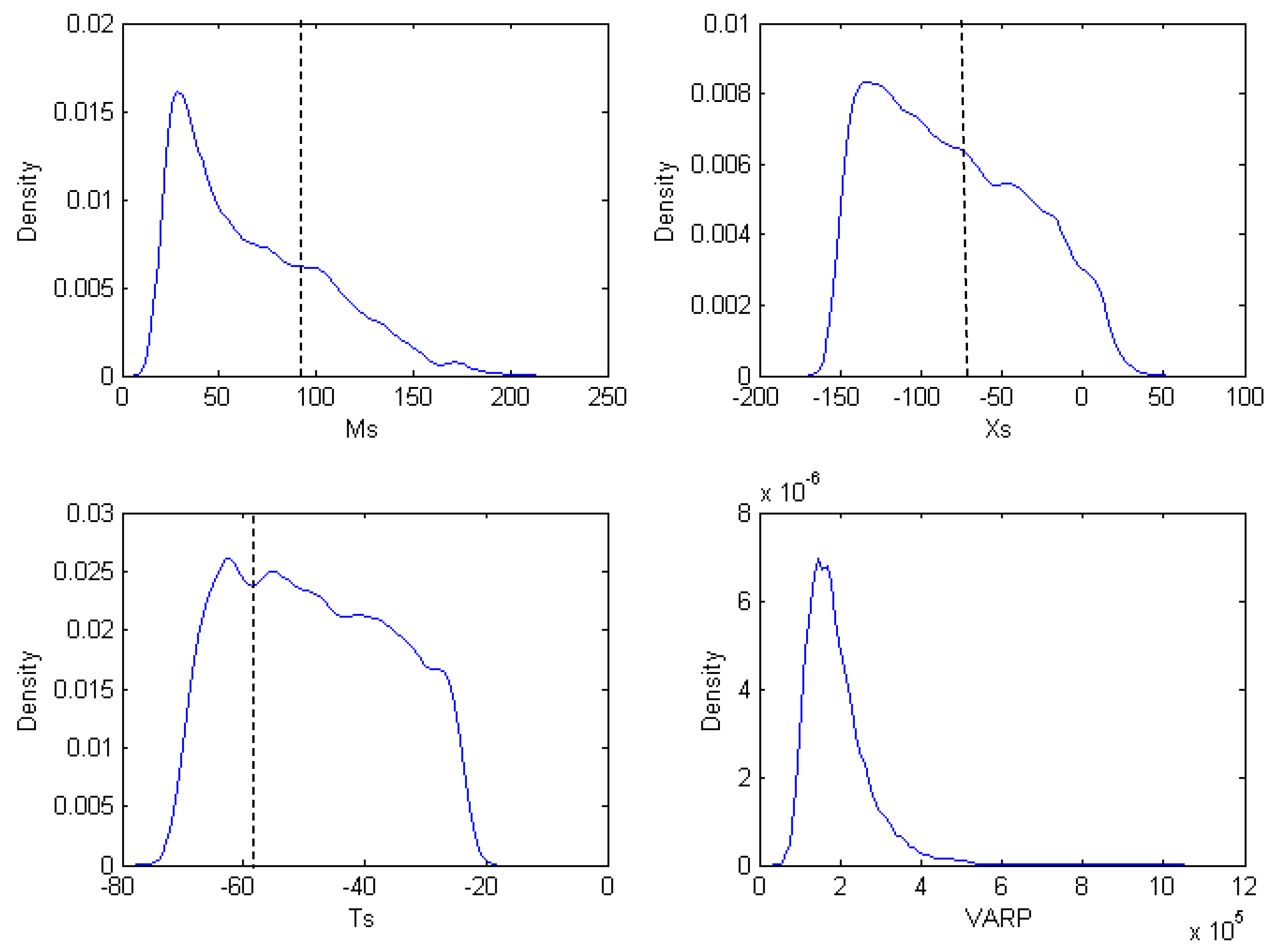
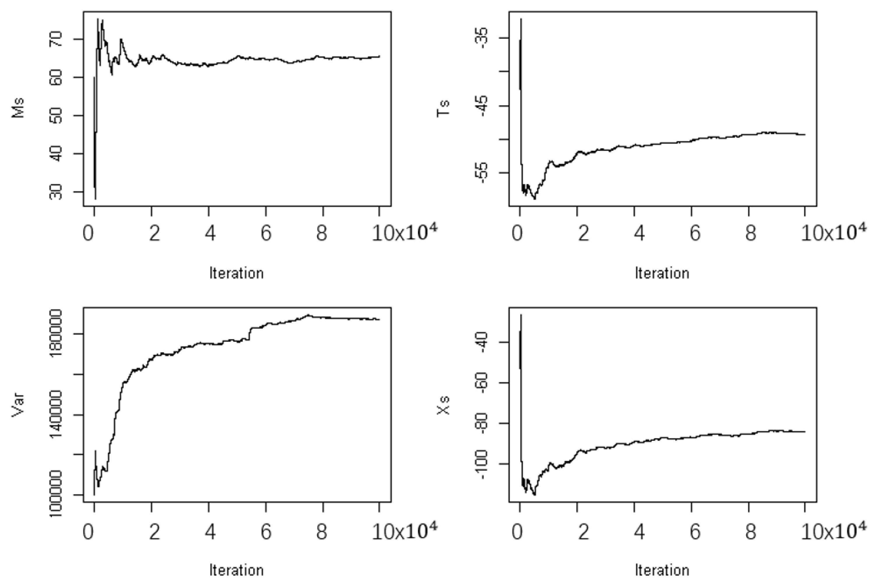
The summary statistics of the results based on the modular-Bayesian inversion are shown in Table 3 and Figure 4, and the posterior distributions of source parameters are shown in Figure 5 and Figure 6. The running mean value of the source parameter is shown in Figure 7. The convergence process of the parameter run means it became more unsteady in the late stage, and σ2 has a slower convergence speed (Figure 7).
Estimated source parameters are relatively close to real values, and the standard deviations are also relatively small. It demonstrates that the modular-Bayesian approach appropriately succeeded in such a complex real case, despite not being perfect. The results also indicate that the results from the heteroscedastic assumption slightly outweigh the results by homoscedastic assumption (Figure 4). They have the same size of errors on release time inversion, but nevertheless have different sizes for inversion on pollutant load and release time.
Taking Run 1 for instance, pollutant load Ms has the largest error among source parameters, and it is approximately 25 tons less than the real amount of released nitrobenzene. This can, to some extent, account for the deviation of the breakthrough curves (BTCs) observed (Figure 3) from hypothetical simplification of forward model as Equation (21). Estimated release location is close to the real release point. However, this deviation presents different directions compared with our unreported studies on some tracer experiment cases. The released time estimated is 10 h earlier than the true release moment. Bayes intervals indicate that Ms and Xs have more uncertainty to Ts.
We can argue for those non-perfect results based on the following reasons. The reason is probably that the hydraulic conditions of the study area are more complex than the forward model. The scale is as large as several hundreds of kilometers. A wide river cross-section led to a longer time for completing lateral mixing. If reconstructing the release history, i.e., L(s) in Section 2.1, a more elaborate forward model should be used, such as the 2D unsteady segmentation model. In addition, nitrobenzene is not completely soluble in the initial river reach after the release, such as the inaccuracy of first order decay kinetics. Even though, more complex models are not easily accessible and tend to be more expensive in practice.
Generally speaking, the posterior PDFs for both Run 1 and Run 2 present a skewed and smooth status (Figure 5 and Figure 6). Long right tails are all present, except the PDF of Ms in Run 2. However, differences are significant for the posterior PDFs between Run 1 and Run 2, especially for Ms and Ts. In Run 1, the skewness of Ms PDF is large and the Ts PDF shows an obvious plateau, while in Run 2, the skewness of Xs is significant and the Ms PDF shows a plateau.
Run 2 seems slightly better than the homoscedastic based Run 1. It indicates to some degree that the heteroscedastic assumption is more acceptable for such a real case. In fact, the distribution styles of monitoring errors at each section are possibly more different; they are tens of kilometers away from each other.

4. Discussion

The Bayesian paradigm of estimation and inference is growing increasingly popular in natural resource management problems and one of its major strengths is the ability to incorporate expert knowledge and opinion in the form of prior probability distributions. However, this strength is not fully exploited in the study. We used the most straightforward uniform probability model throughout for simplicity in practice. It is worth investigating the sensitivity and desirability of using more sophisticated prior probability models and indicating how these capture ‘expert’ opinion or prior belief about the source of a pollution incident (rarely is it the case that environmental agencies and people with local knowledge are ignorant as to the source and timing of an unlawful chemical discharge).
Some may be concerned with the use of uniform prior distributions in that the results of the Bayesian analysis will differ very little from those obtained from more conventional measurement error models. This aspect needs to be investigated and addressed before claims of superiority of the Bayesian approach can be made.
The error terms in Section 2.2 may take more consideration. For example, there are potentially three error components: (1) model mis-specification (non-random); (2) observational and measurement error; and (3) purely random/stochastic error. In addition, for simplicity, we assume an independent distribution of all the observation errors σ o b s , i and model errors σ m o d e l , i . It is not easy to prove this assumption in general if only tested with field data.
In the practice of surface water quality management, some future improvements can be made for this study. Firstly, it is necessary to conduct more case studies based on field work and different release and monitoring scenarios. For the uncertainty analysis, to be used in an emergency response, a simple forward model is sufficient and preferred [50]. How to establish an optimal emergency monitoring network for quickly identifying and recovering pollution source information is an interesting and important question worthy of investigation. To be used for environmental forensics in the aftermath of a spill incident, more sophisticated hydrodynamic and water quality models are required to reconstruct a detailed source release history and pollutant transport processes, i.e., exposure history. A more robust monitoring plan should be developed in advance. Moreover, it seems to be more complex for non-point source pollutant incidents, e.g., pesticides and chemical fertilizer pollution induced by heavy rainfall in agriculture areas. All in all, modular-Bayesian approaches do provide promising and useful tools in many circumstances of watershed management, but more studies still need to be done for developing a sound technique in practice.

5. Conclusions

More and more attention has been paid to the application of the Bayesian method in the estimation of surface water pollution parameters. However, few papers directly apply this method to the source term estimation of actual river pollution. In this work, a model-based Bayesian approach was developed for source identification in response to chemical spill incidents. Self-adaptive MCMC was used to capture the marginal probability distribution of likelihood functions. A reconstructed source inversion scenario based on a historical Songhua River nitrobenzene spill incident was first tested using a modular-Bayesian approach. The results were acceptable for such a large-scale case and under complex circumstances. The inverse uncertainties of each source parameter were depicted as well. The likelihood function and the parameter setting of the AM sampling algorithm of the posterior PDF can be referred to by other spill cases in practice. This paper illustrated that the modular Bayesian based approach is an effective alternative in practice for river pollution source identification. More technique details of the application of Bayesian framework are worthy of being tested and proved, such as to incorporate expert knowledge and opinion in the form of prior probability distributions. Further studies on emergency monitoring network optimization and forward model calibration are also significant.

Author Contributions

Conceptualization, J.J., Y.C.; methodology, software, validation, formal analysis, J.J.; investigation, J.J., Y.C., B.W.; writing—original draft preparation, J.J.; writing—review and editing, J.J., Y.C., B.W.; supervision, J.J.; project administration, J.J.; funding acquisition, J.J., Y.C.

Funding

This work was supported by Special Funds of Shenzhen Water Science and Technology Development (Grant SZCG2018160615), China Postdoctoral Science Foundation (Grant 2014M551249), and National Natural Science Foundation of China (Grant 51509061).

Acknowledgments

We thank professor Ashish Sharma for suggestions on the study and Bin Shi for editing and corrections. We are grateful to the anonymous reviewers and journal editors for helpful comments and suggestions to improve the quality of paper.

Conflicts of Interest

The authors declare no conflict of interest.

References

  1. Camp, J.S.; LeBoeuf, E.J.; Abkowitz, M.D. Application of an enhanced spill management information system to inland waterways. J. Hazard. Mater. 2010, 175, 583–592. [Google Scholar] [CrossRef]
  2. Xue, P.; Zeng, W. Trends of environmental accidents and impact factors in China. Front. Environ. Sci. Eng. China 2011, 5, 266–276. [Google Scholar] [CrossRef]
  3. Yao, H.; Zhang, T.Z.; Liu, B.; Lu, F.; Fang, S.R.; You, Z. Analysis of Surface Water Pollution Accidents in China: Characteristics and Lessons for Risk Management. Environ. Manag. 2016, 57, 868–878. [Google Scholar] [CrossRef]
  4. Ying, A.N.; Sheng-Cai, L.I. Statistics of environmental events in China during the period from January to February in 2013. J. Saf. Environ. 2013, 13, 280–284. [Google Scholar]
  5. Keller, J. Inverse Problems. Am. Mathmatical Mon. 1976, 83, 107–118. [Google Scholar] [CrossRef]
  6. Atmadja, J.; Bagtzoglou, A.C. Pollution Source Identification in Heterogeneous Porous Media. Water Resour. Res. 2001, 37, 2113–2125. [Google Scholar] [CrossRef]
  7. Liu, X.; Yao, Q.; Xue, H.; Zhu, K.; Hu, J. Advance in inverse problems of environmental hydraulics. Adv. Water Sci. 2009, 20, 885–893. [Google Scholar]
  8. Hamdi, A.; Mahfoudhi, I. Inverse source problem in a one-dimensional evolution linear transport equation with spatially varying coefficients: Application to surface water pollution. Inverse Probl. Sci. Eng. 2013, 21, 1007–1031. [Google Scholar] [CrossRef]
  9. Ma, D.; Tan, W.; Zhang, Z.; Hu, J. Parameter identification for continuous point emission source based on Tikhonov regularization method coupled with particle swarm optimization algorithm. J. Hazard. Mater. 2017, 325, 239–250. [Google Scholar] [CrossRef]
  10. Chen, Y.; Wang, P.; Jiang, J.; Guo, L. Contaminant point source identification of rivers chemical spills based on correlation coefficients optimization method. China Environ. Sci. 2011, 31, 1802–1807. [Google Scholar]
  11. Cheng, W.P.; Jia, Y. Identification of contaminant point source in surface waters based on backward location probability density function method. Adv. Water Resour. 2010, 33, 397–410. [Google Scholar] [CrossRef]
  12. Boano, F.; Revelli, R.; Ridolfi, L. Source identification in river pollution problems: A geostatistical approach. Water Resour. Res. 2005, 41. [Google Scholar] [CrossRef]
  13. Wei, G.; Chi, Z.; Yu, L.; Liu, H.; Zhou, H. Source identification of sudden contamination based on the parameter uncertainty analysis. J. Hydroinform. 2016, 18, 919–927. [Google Scholar] [CrossRef]
  14. Zhang, J.; Liu, P.; Wang, H.; Lei, X.; Zhou, Y. A Bayesian model averaging method for the derivation of reservoir operating rules. J. Hydrol. 2015, 528, 276–285. [Google Scholar] [CrossRef]
  15. Shao, D.; Yang, H.; Xiao, Y.; Liu, B. Water quality model parameter identification of an open channel in a long distance water transfer project based on finite difference, difference evolution and Monte Carlo. Water Sci. Technol. 2014, 69, 587–594. [Google Scholar] [CrossRef]
  16. Marshall, L.; Nott, D.; Sharma, A. A comparative study of Markov chain Monte Carlo methods for conceptual rainfall-runoff modeling. Water Resour. Res. 2004, 40. [Google Scholar] [CrossRef]
  17. Hassan, A.E.; Bekhit, H.M.; Chapman, J.B. Using Markov Chain Monte Carlo to quantify parameter uncertainty and its effect on predictions of a groundwater flow model. Environ. Model. Softw. 2009, 24, 749–763. [Google Scholar] [CrossRef]
  18. Keats, A.; Yee, E.; Lien, F.-S. Bayesian inference for source determination with applications to complex urban environment. Atmos. Environ. 2007, 41, 465–479. [Google Scholar] [CrossRef]
  19. Zhu, S. Research on the inverse problems of environmental hydraulics based on Bayesian inference. Ph.D. Thesis, Zhejing University, Hangzhou, China, 2008. [Google Scholar]
  20. Wang, H.; Harrison, K.W. Bayesian Update Method for Contaminant Source Characterization in Water Distribution Systems. J. Water Resour. Plan. Manag. 2013, 139. [Google Scholar] [CrossRef]
  21. Wu, L. Dilemmas downstream from the Songhua River spill. J. Med Toxicol. 2006, 2, 112–113. [Google Scholar] [CrossRef] [Green Version]
  22. Scales, J.A.; Tenorio, L. Prior information and uncertainty in inverse problems. Geophysics 2001, 66, 389–397. [Google Scholar] [CrossRef] [Green Version]
  23. Ntzoufras, I. Bayesian Modeling Using WinBUGS; John Wiley & Sons: Hoboken, NJ, USA, 2009; p. 492. [Google Scholar]
  24. Bates, B.C.; Campbell, E.P. A Markov Chain Monte Carlo Scheme for parameter estimation and inference in conceptual rainfall-runoff modeling. Water Resour. Res. 2001, 37, 937–947. [Google Scholar] [CrossRef]
  25. Box, G.E.P.; Cox, D.R. An analysis of transformations. J. R. Stat. Soc. 1964, 26, 211–252. [Google Scholar] [CrossRef]
  26. Sakia, R.M. The Box-Cox Transformation Technique: A Review. J. R. Stat. Society. Ser. D (Stat.) 1992, 41, 169–178. [Google Scholar] [CrossRef]
  27. Thyer, M.; Kuczera, G.; Wang, Q.J. Quantifying parameter uncertainty in stochastic models using the Box-Cox transformation. J. Hydrol. 2002, 265, 246–257. [Google Scholar] [CrossRef]
  28. Wang, Q.J.; Shrestha, D.L.; Robertson, D.E.; Pokhrel, P. A log-sinh transformation for data normalization and variance stabilization. Water Resour. Res. 2012, 48. [Google Scholar] [CrossRef]
  29. Chen, X. Mathmatical Statistics; Press of University of Science and Technology of China: Hefei, China, 2009. [Google Scholar]
  30. Gelman, A. Prior distribution. In Encyclopedia of Environmetrics; El-Shaarawi, A.H., Piegorsch, W.W., Eds.; John Wiley & Sons: Hoboken, NJ, USA, 2002; Volume 3, pp. 1634–1637. [Google Scholar]
  31. Zheng, Y.; Keller, A.A. Understanding Parameter Sensitivity and its Management Implications in Watershed-Scale Water Quality Modeling. Water Resour. Res. 2006, 420, 72–88. [Google Scholar] [CrossRef]
  32. Hastings, W.K. Monte Carlo sampling methods using Markov chains and their applications. Biometrika 1970, 57, 97–109. [Google Scholar] [CrossRef]
  33. Metropolis, N.; Rosenbluth, A.W.; Rosenbluth, M.N.; Teller, A.H.; Teller, E. Equation of State Calculations by Fast Computing Machines. J. Chem. Phys. 1953, 21, 1087–1092. [Google Scholar] [CrossRef] [Green Version]
  34. Geman, S.; Geman, D. Stochastic relaxation, gibbs distributions, and the bayesian restoration of images. IEEE Trans. Pattern Anal. Mach. Intell. 1984, 6, 721–741. [Google Scholar] [CrossRef]
  35. Link, W.A.; Barker, R.J. Chapter 4—Calculating Posterior Distributions A2. In Bayesian Inference; Barker, R.J., Ed.; Academic Press: London, UK, 2010; pp. 47–74. [Google Scholar] [CrossRef]
  36. Haario, H.; Saksman, E.; Tamminen, J. An adaptive Metropolis algorithm. Bernoulli 2001, 7, 223–242. [Google Scholar] [CrossRef]
  37. Cowles, M.K.; Carlin, B.P. Markov chain Monte Carlo convergence diagnostics: A comparative review. J. Am. Stat. Assoc. 1996, 91, 883–904. [Google Scholar] [CrossRef]
  38. Gelman, A.; Rubin, D.B. Inference from Iterative Simulation Using Multiple Sequences. Stat. Sci. 1992, 7, 457–472. [Google Scholar] [CrossRef]
  39. Raftery, A.; Lewis, S. How Many Iterations in the Gibbs Sampler? Oxford University Press: Oxford, UK, 1970; Volume 4. [Google Scholar]
  40. Fu, W.J.; Fu, H.J.; Skott, K.; Yang, M. Modeling the spill in the Songhua River after the explosion in the petrochemical plant in Jilin. Environ. Sci. Pollut. Res. 2008, 15, 178–181. [Google Scholar] [CrossRef]
  41. Jiang, J.; Wang, P.; Lung, W.-S.; Guo, L.; Li, M. A GIS-based generic real-time risk assessment framework and decision tools for chemical spills in the river basin. J. Hazard. Mater. 2012, 227, 280–291. [Google Scholar] [CrossRef]
  42. UNEP. Awareness and Preparedness for Emergencies on a Local Level (APELL). Chinese River Contamination Resulting from a Petrochemical Explosion and Toxic Spill. 2005. Available online: http://www.unep.fr/pc/apell/disasters/china_harbin/info.htm (accessed on 19 August 2019).
  43. Fischer, H.B.; List, E.J.; Koh, R.C.Y.; Imberger, J.; Brooks, N.H. Chapter 5—Mixing in Rivers. In Mixing in Inland and Coastal Waters; Academic Press: San Diego, CA, USA, 1979; pp. 104–147. [Google Scholar] [CrossRef]
  44. Zhu, B. Application of unsteady flow principle in the study of pollution in the second songhua river. Water Resour. Hydropower Northeast China 1993, 1993, 44–48. [Google Scholar]
  45. Alizadeh, M.J.; Kavianpour, M.R.; Danesh, M.; Adolf, J.; Shamshirband, S.; Chau, K.-W. Effect of river flow on the quality of estuarine and coastal waters using machine learning models. Eng. Appl. Comput. Fluid Mech. 2018, 12, 810–823. [Google Scholar] [CrossRef] [Green Version]
  46. Wu, C.L.; Chau, K.W. Mathematical model of water quality rehabilitation with rainwater utilisation: A case study at Haigang. Int. J. Environ. Pollut. 2006, 28, 534–545. [Google Scholar] [CrossRef]
  47. Chau, K.W.; Jiang, Y.W. Three-dimensional pollutant transport model for the Pearl River Estuary. Water Res. 2002, 36, 2029–2039. [Google Scholar] [CrossRef]
  48. Olyaie, E.; Banejad, H.; Chau, K.-W.; Melesse, A.M. A comparison of various artificial intelligence approaches performance for estimating suspended sediment load of river systems: A case study in United States. Environ. Monit. Assess. 2015, 187, 189. [Google Scholar] [CrossRef]
  49. Chen, X.Y.; Chau, K.W. A Hybrid Double Feedforward Neural Network for Suspended Sediment Load Estimation. Water Resour. Manag. 2016, 30, 2179–2194. [Google Scholar] [CrossRef]
  50. Shamshirband, S.; Jafari Nodoushan, E.; Adolf, J.E.; Abdul Manaf, A.; Mosavi, A.; Chau, K.-W. Ensemble models with uncertainty analysis for multi-day ahead forecasting of chlorophyll a concentration in coastal waters. Eng. Appl. Comput. Fluid Mech. 2019, 13, 91–101. [Google Scholar] [CrossRef]
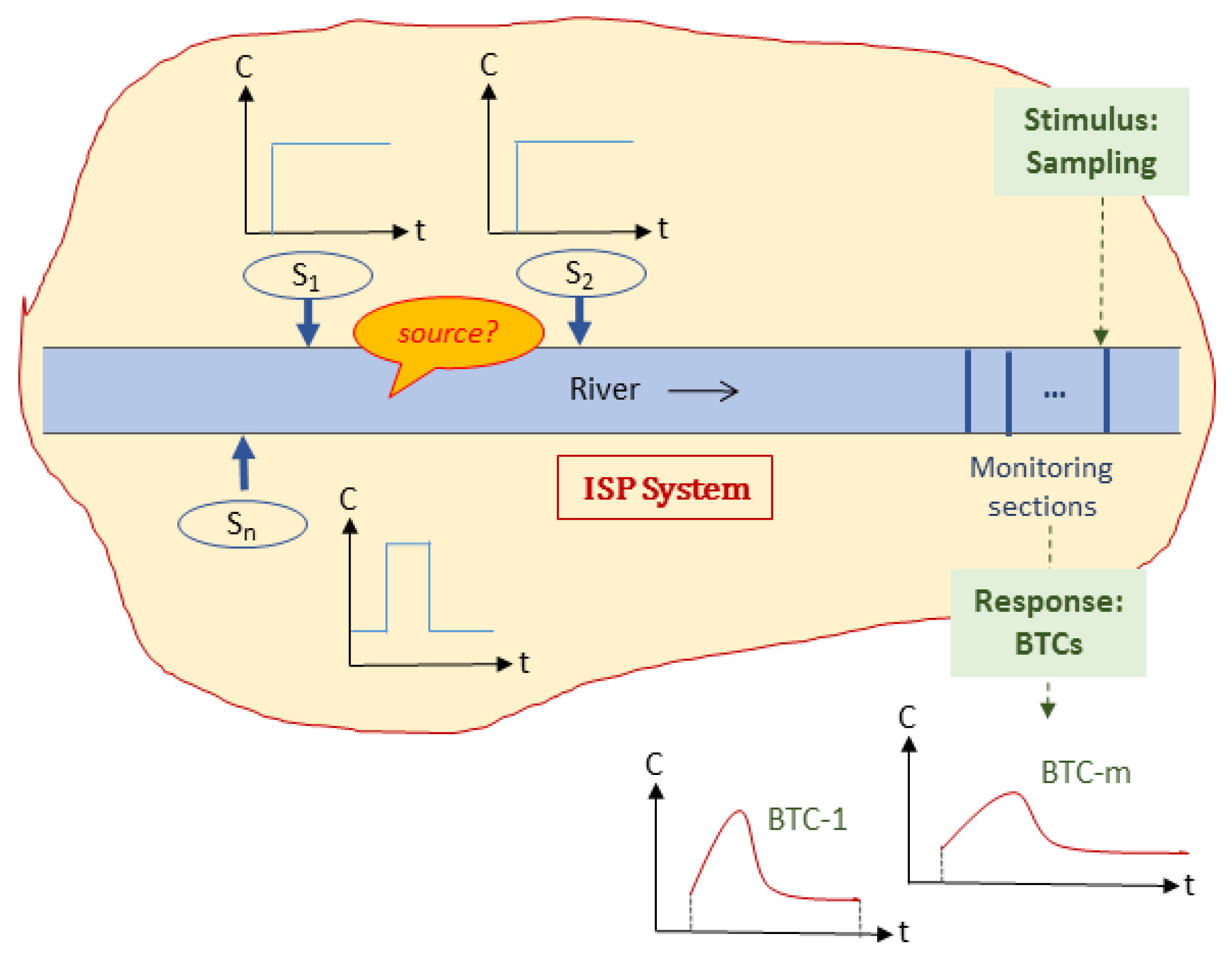
Figure 1. Scheme of the inversion source problem toward river spills from a system theory point of view. Note: C—concentration; S—source; ISP—inversion source problem; BTC—breaking through curves.
Hydrology 06 00074 g001
Figure 2. The Songhua River nitrobenzene spill incident occurred in 2005.
Hydrology 06 00074 g002
Figure 3. Nitrobenzene concentrations at four emergency monitoring sections during the chemical spill incidents.
Hydrology 06 00074 g003
Figure 4. Comparison of the inverse source parameters based on different likelihood functions.
Hydrology 06 00074 g004
Figure 5. Posterior probability density functions with assumptions of homoscedastic errors (Run 1) Dashed lines denote the real values.
Hydrology 06 00074 g005
Figure 6. Posterior probability density functions with assumptions of heteroscedastic errors (Run 2). Dashed lines denote the real values.
Hydrology 06 00074 g006
Figure 7. Running means of the source parameters (Run 1).
Hydrology 06 00074 g007
Table 1. Source and model parameter information for the case of the Songhua River spill.
ParameterValueUnitsReferenceNotes
Ms~92tons[33], UNEP Report [35]Nitrobenzene
xs−75kmUNEP Report [35]#10 north outlet pipeline of the Jilin Petrochemical Plant
ts−58hUNEP Report [35]14:00, 13 November 2005
U3.6km/hassumed by historical hydrology statistics [44]1.00 m/s
Dx0.18km2/htypical value; Fisher formula500 m2/s
A1.6 × 10−3km2measured on GIS map400 × 4 m
K0.001325h−1as estimated in [33]0.0318 day−1
Table 2. The Adaptive Metropolis (AM) algorithm parameter settings.
ParametersSymbolRun 1Run 2
ErrorHomoscedastic,
uncorrelated
adopt this assumption
Heteroscedastic,
uncorrelated
λ1,
λ2
λ1 = 0;
λ2 = 0.35
AMNumber of iterationsnIter100,000same
Initial source parameter values (Ms, Xs, Ts, σ2)S0[60, −50, −40, 105][80, −80, −48, 40]
Proposal scaling factorsd0.30.25
Epsilonε1 × 10⁻¹⁶same
First i0 iterations for fixed covariance C0i00.05 × nItersame
Initial variation of parameters (Ms, Xs, Ts, σ2)varParm[400, 400, 200, 1 × 10⁸][400, 400, 200, 100]
Initial covariance matrixB00.5 × varParm × I3
(I3 is a unit matrix)
same
Parameter constrictionconst.Ms:[20, 200]
Xs:[−200, 5]
Ts:[−72, −24]
same
Table 3. Summary statistics of the inverse results at the Songhua River.
Real ValuesMeanSDSkewnessP0.025P0.5P0.975Bayes Interval *
Likelihood Function Defined by Equation (11), Homoscedastic # (Run 1)
Ms (ton)9267.237.80.77621.558.0152[20, 122]
Xs (km)−75−80.945.90.346−147−86.48.38[−150, −14]
Ts (h)−58−48.212.90.146−68.6−49.0−25.3[−68, −28]
σ2 (mg2/L2) 1.95 × 1058.9 × 1043.0169.30 × 1041.76 × 1053.98 × 105[8.28 × 10⁴, 2.99 × 10⁵]
Likelihood Function Defined by Equation (12), Heteroscedastic (Run 2)
Ms (ton)9211451.2−0.08125.7116196[42.0, 200]
Xs (km)−75−69.348.6.00.488−142−76.433.7[−147, 3.5]
Ts (h)−58−51.413.00.307−71.0−52.9−26.2[−72.0, −32.3]
σ2 (mg2/L2) 0.211.11.47515.228.157.4[14.0, 45.6]
Note: SD denotes standard deviation, P0.025 denotes 0.025 quantiles of cumulative distribution. * Highest probability density intervals at α = 0.1 # The last 60,000 samples were used for Run 1, and the last 80,000 samples were used for Run 2.