A Novel Approach for the Integral Management of Water Extremes in Plain Areas

Abstract

Due to the socioeconomical impact of water extremes in plain areas, there is a considerable demand for suitable strategies aiding in the management of water resources and rainfed crops. Numerical models allow for the modelling of water extremes and their consequences in order to decide on management strategies. Moreover, the integration of hydrologic models with hydraulic models under continuous or event-based approaches would synergistically contribute to better forecasting of water extreme consequences under different scenarios. This study conducted at the Santa Catalina stream basin (Buenos Aires province, Argentina) focuses on the integration of numerical models to analyze the hydrological response of plain areas to water extremes under different scenarios involving the implementation of an eco-efficient infrastructure (i.e., the integration of a green infrastructure and hydraulic structures). The two models used for the integration were: the Soil and Water Assessment Tool (SWAT) and the CELDAS8 (CTSS8) hydrologic-hydraulic model. The former accounts for the processes related to the water balance (e.g., evapotranspiration, soil moisture, percolation, groundwater discharge and surface runoff), allowing for the analysis of water extremes for either dry or wet conditions. Complementarily, CTSS8 models the response of a basin to a rainfall event (e.g., runoff volume, peak flow and time to peak flow, flooded surface area). A 10-year data record (2003–2012) was analyzed to test different green infrastructure scenarios. SWAT was able to reproduce the waterflow in the basin with Nash Sutcliffe (NS) efficiency coefficients of 0.66 and 0.74 for the calibration and validation periods, respectively. The application of CTSS8 for a flood event with a return period of 10 years showed that the combination of a green infrastructure and hydraulic structures decreased the surface runoff by 28%, increased the soil moisture by 10% on an average daily scale, and reduced the impact of floods by 21% during rainfall events. The integration of continuous and event-based models for studying the impact of water extremes under different hypothetical scenarios represents a novel approach for evaluating potential basin management strategies aimed at improving the agricultural production in plain areas.

1. Introduction

Floods and droughts are the two main types of natural disasters causing major socioeconomic losses around the globe. Some examples are those described by [1] for America, [2] for Asia, [3] for Europe and, at a global scale, by [4,5,6]. Furthermore, extreme hydrologic events generate negative impacts on ecosystems, interfering with hydrological connectivity [7], the nitrogen cycle [8], causing cyanobacterial blooms [9] and alterations in aquatic habitat availability [10], among others. Likewise, the agriculture and livestock production are also impacted by water extremes [11,12], along with the local population [13,14]. The frequency, magnitude and distribution in space and time of floods and droughts have increased in many regions around the world [2,15]. According to the Intergovernmental Panel on Climate Change’s (IPCC) fifth report, extreme hydrologic events are expected to globally increase due to climate change [16,17]. For these reasons, the characterization of hydrologic extremes and the development of mitigation measures are vital for proper risk management [18]. [19] predicted that by 2030 more than 250% of the urban land would suffer droughts or floods. This prediction is of great concern, especially for Latin America due to the high vulnerability of its population [20].

Plain areas are characterized as having a high potential for agriculture and livestock production, as well as for urban development [21,22,23,24]. Fluctuations in the rainfall regime in plain areas where rainfed agriculture is the main productive activity could exert profound negative effects in the local economies due to drops in the crop yields [25,26,27]. Rainfed agriculture constitutes 80% of the total cultivated land around the world, and it is responsible for 60% of the global crop yield [28]. The Pampas ecoregion in Argentina is a broad grassy plain located in the Central Eastern part of Argentina [29]. Many of the negative socioeconomical impacts on the local agriculture and livestock production are associated with climate variability [30,31]. Droughts in this region have worse consequences than floods. According to [32], the estimated economic losses in the agricultural sector resulting from an extreme drought in 2008 were higher than $700 million dollars, whereas [33] Latrubesse and Brea (2009) reported losses of up to $570 million dollars for extreme floods occurring in the same region. Furthermore, [34] pointed out that, at a global scale, droughts and floods have different spatio-temporal impacts: whereas floods last hours to days and their spatial distribution is relatively small (i.e., up to 250,000 km²), droughts affect larger areas (i.e., up to 25,000,000 km²) and last longer, from months to years. As explained further below, this could not be precisely the case for the Pampas region.

One of the economic and productive sectors most affected by water extremes in the Pampas plains is agriculture, which largely depends on the soil humidity [35,36,37]. This situation is linked to the shallowness of the aquifer, a common characteristic for the whole region. During wet periods, the aquifer level reaches the surface and saturates the soil profile with water [31,38]. This translates into a reduction in crop yields. During the dry seasons, when rainfall diminishes and evapotranspiration increases, the soil humidity rapidly drops, along with the phreatic level. During droughts, crops are subjected to stressful conditions, growth rates are reduced, and consequently their biomass and yield decrease. If the condition persists, crops could be entirely lost [39].

Floods in the Pampas region are characterized as covering large surface areas (e.g., approximately 140,000 km² in 2012, as reported by [38] and as lasting for long periods of time, from a few days to months. Several factors influence the phenomena: (I) the occurrence of rainfall extreme events; (II) a phreatic level raise, with the water table reaching the surface; (III) a surface runoff stagnation due to the reduced land slope; (IV) a poorly defined drainage network; and (V) a low hydraulic capacity of channels. All these factors influence the surface runoff dynamics, making them acquire a mantle-shaped pattern [40,41]. Altogether, these factors make flooding events more extreme in these areas, with large water volumes moving with a low energy and covering large surface areas not exceeding 1 m in depth. These types of systems are known as “non-typical hydrological systems” (NHS) because there is surface water movement across basin boundaries or because basin boundaries change as the water level fluctuates [42].

Droughts can be classified into several categories: meteorological, agricultural, hydrologic and socioeconomic [43,44,45]. Droughts in the Pampas region may have increased over time due to changes in land use that were forced by the conversion from natural grasslands to a rainfed agriculture [30] and due to a rainfall reduction conditioned by the activity of the South Atlantic anticyclone and its interaction with a continental depression within the Pampas region known as the humid Pampas [32]. In the Pampas region, droughts begin with a reduction in the precipitation rate to below average and an increase in the evapotranspirative demand (meteorological drought). Furthermore, there is a sharp decrease in the soil humidity (agricultural drought), as well as in the aquifer water level. During dry periods when the aquifer water level drops, the stream water level descends and even channels dry, favored by their already-shallow depths (hydrologic drought). In 2008, 470,000 km² of the Pampas region were affected by a drought that lasted almost two years [32]. Serious crop yield losses occurred during this period. Crops in the region are mainly dominated by soybean, corn, wheat and sunflower. Likewise, losses in the cattle farming sector also occur (socioeconomic drought).

Predicting hydrological responses is a major challenge in water resources management, especially when that water involves the irrigation of crops, raising early warnings or preparing for floods, as well as assuring hydroelectric power generation, among others. Currently, different approaches have been developed for better predictions by means of the use of modelling techniques. Some examples are the development of an enhanced extreme learning machine model for river flow forecasting [46], a support vector regression (SRV) model and a hybrid SVR-based firefly algorithm model to simulate evaporation [47], the grading of the eutrophic state of a reservoir using an Environmental Fluid Dynamics Code (EFDC) model [48], a model for sea-bottom change simulations in coastal areas with complex shorelines [49], a model for turbulent fluvial systems [50], a decision-making model for reservoir flood control [51] and the coupling of hydrologic and hydraulic models for modelling floods [52].

Numerical models constitute useful tools for analyzing the hydrologic response of a basin to water extremes and the impacts caused by them. These models could be classified as continuous or event-based, depending on the set-up (as defined by [53]). Continuous models help understand processes related to the water balance (e.g., evapotranspiration, soil moisture, percolation, groundwater discharge and surface runoff), allowing for the analysis of water extremes for either dry or wet conditions. Complementarily, event-based models aid in knowing the response of a basin to a rainfall event (e.g., runoff volume, peak flow and time to peak flow, flooded surface area) [54].

The integration of continuous and event-based hydrologic-hydraulic models [55,56,57] can help evaluate the dynamics in the water balance of a basin and quantify its hydrologic response under different hypothetical scenarios before deciding on the implementation of management strategies for water extremes. Some examples are the integration of the Soil and Water Assessment Tool (SWAT) with the storm event Dynamic Watershed Simulation Model (DWSM) [58], the integration of MIKE Système Hydrologique Européen (MIKE SHE) with MIKE 11 [59], the integration of the Modelo de Grandes Bacias–Instituto de Pesquisas Hidráulicas (MGB-IPH) with the Hydrologic Engineering Center–River Analysis System (HEC-RAS) hydraulic model [60] and the integration of the Hydrologic Modeling System (HEC-HMS) with HEC-RAS [61,62].

Among the available open-source models, we chose integrating SWAT [63] with CTSS8 [64]. The former is a continuous hydrologic model, whereas the latter is an event-based hydrologic-hydraulic model. The advantages of using SWAT rely on its capability for analyzing (using a continuous approach) the hydrologic response of a basin during dry or wet periods, taking into account the existing land use and management practices. Despite SWAT having been reported as underestimating peak flows [58], CTSS8 reproduces them accurately, and it is suitable for modelling hydrological processes. Moreover, due to this quasi-2D model being based on the discharge laws from the kinematic and diffusive approaches of the momentum equation, it is especially adapted for analyzing the multidirectional dynamics of the surface runoff, a common characteristic of plain areas. The CTSS8 model has been satisfactorily used at basins located in plain areas such as the Ludueña Basin [64,65] and the lower Paraná Delta [66,67].

In general, the study of droughts and floods has been mostly centered on their characterization and impact assessment. However, due to the complexity of the system, there are few studies that analyze the mitigation strategies. This complexity is given by the heterogeneity of the land uses, soil types, topography, agricultural management practices, water use, and the existence of hydraulic structures in the field.

Understanding the interrelationship among these variables is fundamental when studying the effects of the temporal variation in the precipitation regime. The analysis of hydrologic extremes must take into account the interaction among the climate, land use, types of soils, topography, agricultural practices, presence of hydraulic structures, etc., to improve our understanding of the system’s mode of functioning and to have more efficient management procedures in order to minimize the impacts through proper prevention and mitigation. The integration of hydrologic-hydraulic models would aid in this sense, constituting a useful tool for management purposes. Additionally, an improvement of the political guidelines and governmental programs is needed to regulate the use of ecosystems by the agricultural sector, taking into account the ecosystem’s resilience level and promoting the development and use of an eco-efficient infrastructure [68]. The latter involves the integration of hydraulic structures [69,70,71] with a green infrastructure [72,73,74], which, combined, allow for a more effective control of droughts and floods at a lower cost [75].

Land use management plays a significant role in the propagation of water extremes ([76,77]. Consequently, the agricultural practices based on non-structural methods [78] and the restoration of flood plains that allow for the existence of riparian forests are important green-infrastructure elements [79]. Riparian zones are key interfaces between stream and terrestrial ecosystems [80]. These zones could provide many ecosystem services, including flood and drought control [81], a reduction in soil erosion rates and in the amounts of pesticides and fertilizers reaching the watercourses [82], and the protection of the aquifer recharge zones [83]. These recharge zones are characterized as having a high biodiversity and biomass productivity [84], which are sometimes threatened by the advance of the agricultural frontier.

One of the present challenges in the Pampas region is to quantify the processes causing extreme hydrologic events as a basis for the implementation of an eco-efficient infrastructure. This consists in increasing the soil humidity during dry periods and in reducing the surface runoff during wet periods.

The understanding of surface runoff processes and soil humidity dynamics in plain areas is of vital importance for the management of crops and water. Hence, the study of the anthropic effect on the hydrologic system for plain areas required the use of integrated simulation tools in assisting in diagnosing and planning.

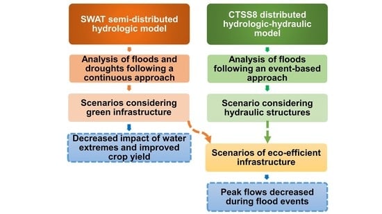
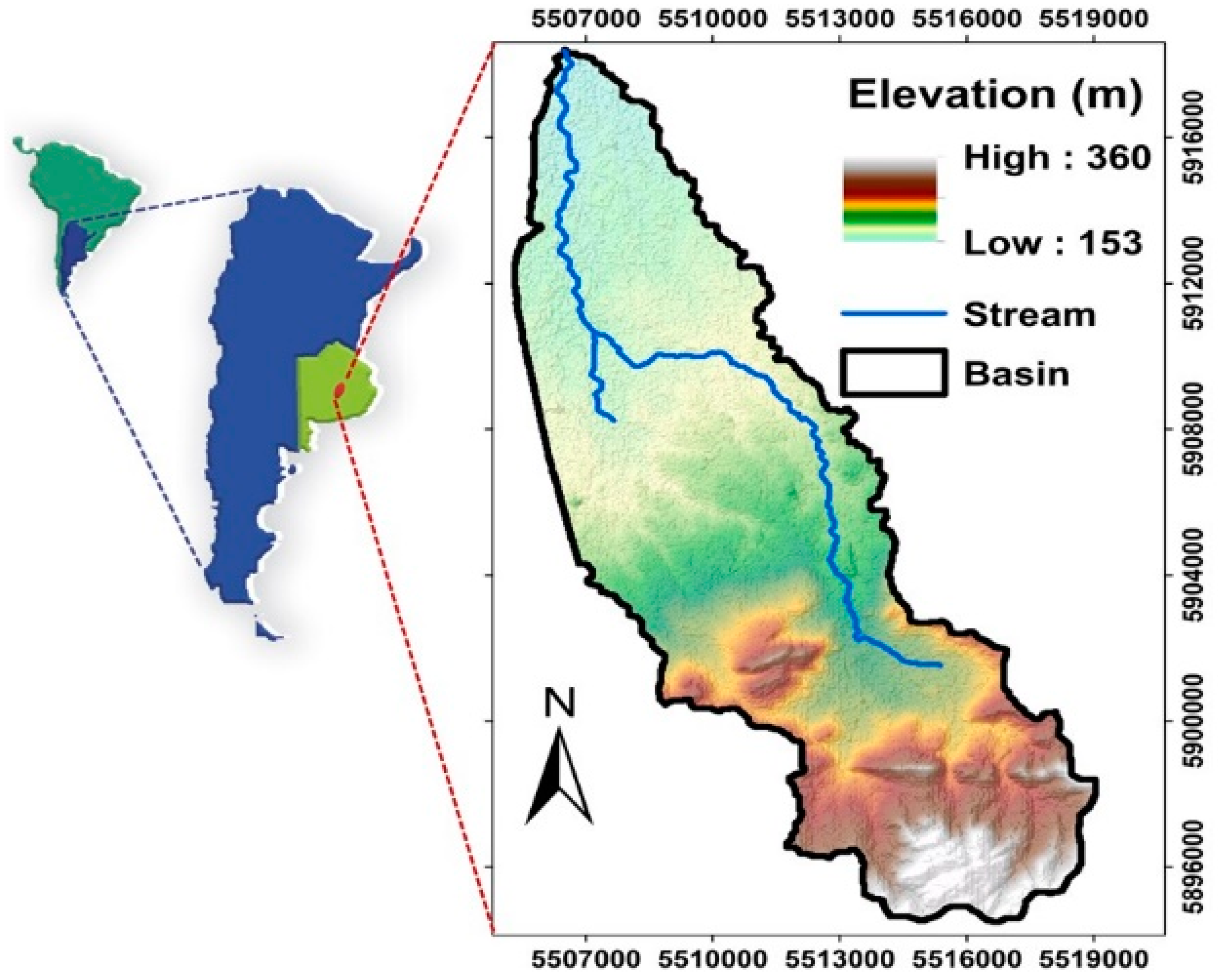
The objective of this article is to evaluate the dynamics in the water balance and to quantify the surface runoff and soil humidity under different hypothetical eco-efficient scenarios, through the integrated application of continuous (i.e., SWAT) and event-based (i.e., CTSS8) hydrologic-hydraulic models. This study was performed in the Santa Catalina stream basin (SCSB) located in the Pampas region of Argentina (see the next section for further information about the study zone).

The novel contribution of our study is that it helps, through the use of integrated models, in finding effective solutions to solve critical hydrologic problems faced by the agricultural and livestock production sectors operating in plain areas (i.e., testing different scenarios of management strategies to find the most effective). An effective intervention based on informed decisions could help minimize the impacts of extreme water events, and prevent or alleviate socioeconomic crises.

Characteristics of the Study Zone

The SCSB (59°79′–59°92′ W and 36°88′–37°10′ S) is located in the center of the Buenos Aires province, Argentina. This basin has a surface area of 13,800 ha. The altitude ranges from 360 to 153 m.a.s.l. (Figure 1). A hilly landscape dominates the upper sector of the basin, whereas the topography flattens toward the middle to lower sectors of the basin, as it transitions downstream into a plain area [85]. In the plain area, vertical water movements (i.e., precipitation, evapotranspiration) and water storage processes of surface and groundwater origin predominate over horizontal water movements (i.e., surface runoff). The groundwater flow follows a northeast direction [86]. The geomorphology of the study area is classified into two domains: the hilly domain (HD) and the extra-hilly domain (EHD) [87]. The HD is located in the upper part of the basin where rocky outcrops belonging to the Tandilia Hills system prevail [88]. It is subdivided into two areas: interfluvial and fluvial valleys. The highest-elevation area of the system has round-shaped hills, with their tops flattened due to aeolian erosion. Most of the basin is within the EHD. This domain is characterized as being mostly flat, with subtle height and slope variations. The EHD could be subdivided into two areas: 1) Aggradation plain with stratified calcareous crust, situated toward the middle part of the basin. This consists of reddish brown, compact, carbonated silts with a calcareous crust (0.5–1 m), above which there is a shallow sedimentary cover (0.5–0.7 m) modified by pedogenesis. The calcareous soil-crust substrate generates surface waterlogging, and deficient internal drainage conditions in the soil profile. 2) Aggradation plain with dominant loess cover, situated in the lower part of the basin and composed of a substrate with calcareous crust and loess cover.

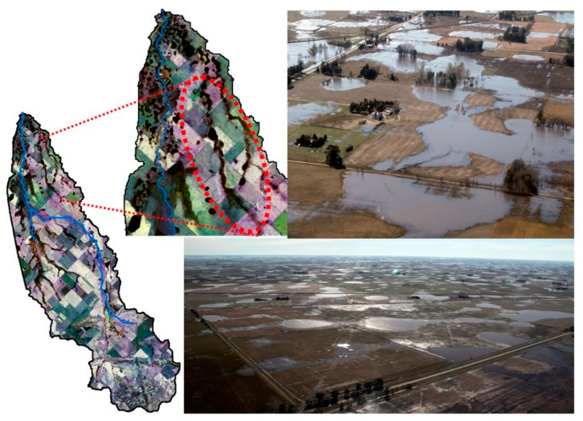
The SCSB is characterized by a landscape shaped by wind action due to the low morphometric potential and the fine granulometry of the soils, which facilitate aeolian transport. The concentrated erosive action of the wind in this area is capable of excavating closed depressions known as deflation hollows, which play a very important role in the water flow and storage. In periods of water excess, the connection of the surface water-storage areas (i.e., the deflation hollows) generate a water flow parallel to the direction of the stream, as seen from the Satellite Pour l’Observation de la Terre (SPOT) image shown in Figure 2.

Figure 3 shows the temporal distribution of dry and wet periods after applying the 12-month standardized precipitation index (SPI) [89,90,91]. The precipitation data came from a weather station located in the basin: the Azul City’s weather station, operated by the National Weather Service of Argentina (SMN). This station has the longest rainfall record for the study area (1901–present). Since the SPI is standardized, the wet and dry periods can be represented at the same scale.

Table 1. Characterization of water extremes at the Santa Catalina stream basin through the use of the 12-month SPI.

Water Extremes	SPI	Frequency (month)	Percentage
Extremely dry	< −2	29	2.1
Severely dry	−2 to −1.5	56	4
Moderately dry	−1.5 to −1	142	10.2
Moderately wet	1 to1.5	146	10.5
Very wet	1.5 to 2	47	3.4
Extremely wet	> 2	43	3

presents the characterization of the hydrologic extremes for the 1901–2015 period. These resulted in 85 months of severe to extremely severe droughts representing 6.1% of the studied period. Very wet to extremely wet periods accounted for 90 months, representing 6.5% of the reporting period, with a total of 1380 monthly-rainfall cases being analyzed.

The most extreme droughts in the SCSB occurred in 1911–1912, 1916–1918, 1924–1926, 1929–1933, 1935–1939, 1942–1943, 1950–1951, 1957, 1962–1963, 1979–1980, 1982–1983, 2008–2009, and 2013–2014. Extremely wet periods in this basin were recorded in 1904, 1908–1909, 1914–1915, 1940, 1946–1947, 1978, 1980–1981, 1986–1987, 1992, 1998, 2000–2003, and 2012–2013. According to many authors [92,93,94,95,96,97], the Pampas region has experienced an increase in precipitation rates since 1960. This reported trend is coincident with the rainfall pattern seen in Figure 3. With an increased precipitation rate, flood events in the basin could be more frequent and intense: This could be enhanced by climate variability and by the demand of agricultural commodities driven by the international market which, to a great extent, determine land use and production practices. The described situation could lead to negative scenarios during water-excess periods in the basin, impacting its economy which, as previously stated, largely depends on land productivity.

2. Methodology

The hydrologic simulation for the SCSB was performed using two different models (Figure 4). One of these models was the Soil and Water Assessment Tool (SWAT). This is a continuous, daily, semi-distributed numerical model that allows the representation of different physical processes in watersheds, in order to analyze the impacts of the land use change in the water balance ([63,98,99]. The referred model estimates the effective rainfall in the basin by means of the curve number (CN) method developed by the Soil Conservation Service of the United States [100]. The aquifer contribution to streamflow is also accounted for by the model and calculated using the linear reservoir method [101]. The resulting runoff, as modelled with SWAT, was used as an input source for the CELDAS8 model (CTSS8) [64,67].

CTSS8 is a hydrologic-hydraulic and event-based model which allows for the simulation of the surface runoff in plain areas where the laminar runoff outweighs the channeled runoff. Using a 2D-spatial configuration, a simulation of the resulting surface runoff dynamics can be performed based on a spectrum of discharge laws from the kinematic and diffusive approaches of the momentum equation, taking into account the water movements through streams, channels and floodplains [65,102].

From the daily water balance modelled with SWAT for the SCSB, the event during which the highest peak flow was observed for the study period (2003–2012) was selected and analyzed as a case study. The selected event was the one that occurred from the 17th to the 25th of May, 2012. This event showed a return period of 10 years.

2.1. Simulation of Scenarios

In order to analyze the water dynamics during extreme hydrologic events in the SCSB, different hypothetical scenarios were tested and contrasted against a baseline scenario. With baseline scenario we imply a scenario considering the currently existing conditions in the basin (for details refer to Section 3.1, “SWAT input data”).

The hypothetical scenarios considered the implementation of a green infrastructure. One of these involves land use change through the implementation of forests of species that could withstand floods and droughts, such as Salix spp. [103,104], both forming riparian forests and covering land depressions. The other green infrastructure scenario incorporates (along with forests) the use of contour farming. These measures would contribute to the slowing down of the surface runoff during floods and would help retain soil humidity during dry periods. The mentioned scenarios were modelled with SWAT.

The existence of hydraulic structures was also considered as another scenario and modelled with CTSS8. These hydraulic structures are meant to regulate and retain the water excess in case extreme events occur.

The integration of the two models (i.e., SWAT and CTSS8) served to analyze different scenarios of land use, agricultural management practices and the existence of hydraulic structures regulating the water passage and soil moisture in wet and dry periods, respectively. The hypothetical scenarios used with each of the two models are further described below.

2.2. Description of the Scenarios Used with SWAT

Two hypothetical scenarios of green infrastructural measures for the management of water extremes were simulated with this semi-distributed model. The baseline scenario was defined beforehand by analyzing the daily water balance for the current land uses. Each one of the hypothetical scenarios is described as follows.

SWT1 Scenario: Implementation of Changes in Land Use

With changes in land use, we refer to beneficial changes that would alleviate or prevent the impacts caused by extreme events. For this scenario, riparian forests were simulated as covering a 100-m strip on each side of the stream. Furthermore, forests were simulated as covering the deflation hollows. These changes are shown in Figure 5. The forested areas in the basin for this scenario increased from 0.4% (59 ha) (baseline scenario) to 6% (806 ha) of the total basin surface area (13,800 ha).

With the implementation of this hypothetical condition, the evaporation could be minimized and the storage of water in the soil profile maximized during periods of drought. These changes in land use (i.e., forested riparian strips and forested deflation hollows) are represented in Figure 5.

SWT2 Scenario: Implementing Crop Best Management Practices along with Changes in Land Use

This scenario implies the use of contour farming as an agricultural management practice combined with the strategies presented for the SWT1 scenario. Contour farming entails planting crops following the elevation contour lines. This management strategy is suitable for soybean, wheat and pasture crops and is recommended for areas with < 3% slopes, such as those existing in SCSB. This practice was applied in areas with soybean, winter wheat and pastures, which in total covered 8562 ha (Figure 5).

2.3. Description of the Scenarios Used with CTSS8

Three hypothetical scenarios and a baseline scenario were used with the CTSS8 model. The baseline scenario considered the SCSB as is (i.e., under the currently existing conditions). The last registered flood in the basin occurred on 5/17/2012. The flood return period for this basin is 10 years.

For the first scenario or scenario CTS1, hydraulic structures were simulated in the field with the purpose of regulating the water flow. Another scenario, called CTS2, considered the implementation of a green infrastructure positively affecting the land use change and crop management practices. Finally, the CTS1 and CTS2 scenarios were combined as CTS3 to analyze the effect of hydraulic structures coupled with green infrastructural measures on the control of water excess.

Details on CTS1 Scenario: Implementation of Hydraulic Structures

This scenario considered embankments (1 × 6 m, height × width) for storing and temporarily delaying surface runoff, and four culverts across the embankments in order to regulate the output flow, each one having a discharge coefficient of 0.3.

Figure 6 shows the location of the embankments and culverts. One of the embankments was positioned on an existing road located in the southeastern portion of the basin. The length of this embankment is 7 km. Another embankment, located north of the former one and having a length of 5 km, was also proposed.

CTS2 Scenario: Implementing Crop Best Management Practices Along with Changes in Land Use

This scenario analyzes the response of the system (i.e., SCSB) to the 5/17/2012 precipitation event, taking into account changes in the land use and the implementation of best management practices for crops. The runoff scenario used as an input source for CTSS8 was previously obtained with SWAT (refer to SWT2 scenario).

CTS3 Scenario: Joint Implementation of CTS1 and CTS2 Scenarios

Scenario CTS3 consists of scenarios CTS1 and CTS2 combined. The hydraulic structures and green infrastructural measures were both integrated to control the water excess as if the 5/17/2012 precipitation event would have occurred under the simulated conditions.

3. Modelling

For the simulations we provided the models with the input data (refer to each model for specifics), including the adjusted parameters (and their respective goodness of fit measures), for the calibration and validation periods.

3.1. SWAT Input Data

The SWAT model needs to be supplied with meteorological and topographic information, along with soil types and land uses. The used data sources are described below:

1- Data from three weather stations with series of daily recorded data (

Table 2. Location of the meteorological stations used for the study.

Station Code	Station Name	Latitude	Longitude	Elevation (m)
1	Azul	−36.832	−59.886	145
2	La Firmeza	−36.973	−59.968	165
3	Siempre Amigos	−37.016	−59.852	190

). The time series ranged from 2003 to 2012.

2- Soil types map: a map developed by the National Institute of Agricultural Technology [105] was used for the study. This map has a 1:50,000 scale. Nine soil types were identified in SCSB (i.e., Argiudolls, Hapludolls and Natracualf, Rock, Natraquolls, Paleudolls), with the three former types being dominant (Figure 7a).

3- Land use map: a map developed by [106] for this basin was employed (Figure 7b). Land cover in the basin is mainly associated with agriculture and cattle farming uses. The categories associated with the latter use are pastures, bermudagrass and crested wheat grass. Agriculture is dominated by rainfed crops such as soybean in summer and wheat in winter. We used crop rotation when modelling the water balance with SWAT, since the basin is cultivated all year round. This was done by applying the “scheduled management operation” option, which allows for setting the dates for “planting/beginning of growing season” and “harvest only operation” [107]. Apart from the above-mentioned, the other listed land use categories were: forest and water.

4- Corrected digital elevation model (DEM): The DEM Shuttle Radar Topography Mission (SRTM) was used [108,109]. This DEM was corrected in a previous study [110] (Figure 7c).

The SWAT hydrological model produced a vector map consisting of 408 hydrological response units (HRUs) that are a combination of land uses, soil types and land slopes. These units are hydrologically similar or homogeneous, and from them the water balance is quantified on a daily scale [63].

3.2. SWAT Model

The SWAT simulation considered a 10-year period of analysis (2003–2012). The 2003–2005 period was used for the model warm-up, the 2006–2010 period was employed for the model calibration and the 2011–2012 period for the model validation.

A sensitivity analysis was performed to determine the most sensitive SWAT model parameters (Figure 8). The software used for this purpose was SWATCUP, which uses the sequential uncertainty fitting algorithm [111]. CN2 (Curve number for moisture condition II) and ESCO (soil evaporation compensation factor) were the most sensitive model parameters, explaining >50% of the variation in the model output. These were followed by SOL_Z (depth from the soil surface to the bottom of the layer), GWQMN (threshold water depth in shallow aquifer for base flow to occur) and SOL_AWC (available water capacity of the soil layer). Due to the extension of the other parameter names, only their abbreviations are shown. Please refer to the SWAT manual (i.e, [107]) for their full names.

Table 3. Most sensitive SWAT model parameters and their range of adjustment for the Santa Catalina stream basin.

Parameter	Description	Method	Range	Value
CN2.mgt	SCS runoff curve number	Relative	±0.25	−20
ESCO.hru	Soil evaporation compensation factor	Replace	0–1	0.1
SOL_AWC.sol	Available water capacity of the soil (mm H2O/mm soil)	Relative	±0.50	30
GWQMN.gw	Aquifer for base flow to occur (mm)	Replace	±5000	600
SOL_Z.sol	Depth from the soil surface to the bottom of the layer (mm)	Relative	±0.30	−5
ALPHA_BF.gw	Base flow alpha factor (days)	Replace	0–1	0.1
REVAPMN.gw	Threshold depth water in shallow aquifer for “revap” to occur (mm)	Replace	0–500	100
SLSUBBSN.hru	Average slope length (m)	Replace	10–1000	1000

presents the eight most sensitive parameters, their description, their calibrated values and the ranges in which the parameters were moved.

As shown in Table 3, the parameters that control the vertical component of the water movement in the soil are the most important ones. CN2 and ESCO were the most sensitive parameters of the model, followed by SOL_Z, GWQMN and SOL_AWC.

According to [63,112], in order to consider the adjustment of a model as being adequate, Nash Sutcliffe (NS) and percent bias (PBIAS) should be within certain intervals: 0.65 < NS ≤ 0.75 and ±10 ≤ PBIAS < ±15. Since our results are within those ranges, we can confirm that our model results are satisfactory (

Table 4. Statistical parameters associated with the calibration (2006–2010) and validation (2011–2012) of the SWAT model using daily data for the Santa Catalina stream basin.

Period	NS	Log (NS)	(R2)	PBIAS
2006–2010	0.66	0.6	0.82	10.4
2011–2012	0.74	0.65	0.86	−14.1

). Due to NS being sensitive to extreme flow values, we used the log(NS) for the model adjustment during low flows [113].

The simulated and the observed hydrographs for the calibration and validation periods are shown in Figure 9. The simulated discharge adequately represented the observed discharge for both the dry and wet periods.

Because there is not enough streamflow data to increase the validation period, the model was validated using the Gravity Recovery and Climate Experiment (GRACE) satellite images, calculating from them the total water storage change [114,115]. The shallow phreatic aquifer in the study zone shows a strong correlation between its level and the water balance processes occurring in the surface (i.e., evapotranspiration, surface runoff and soil moisture) [116]. For this reason, the GRACE images are more suitable for analyzing water extremes in these types of areas, allowing for the estimation of the water storage anomaly in the basin.

The used images have an approximate spatial resolution of 300 km and a monthly time scale. The total water storage change obtained from the GRACE images was compared with the total water storage change simulated with SWAT for the 2006–2012 period (Figure 10). For the estimation of the SWAT total water storage change, we followed the [117] methodology. Despite the small size of SCSB compared to the GRACE image resolution, we observed coincident patterns in the total water storage change between the GRACE and SWAT values.

3.3. CTSS8 Input Data

In order to use the CTSS8, the following information was required:

• Topography of the study area, which was obtained from the SRTM DEM with a second arc spatial resolution. Due to the fact that the CTSS8 interface has a limited number of elements, the DEM resolution was resampled using 200 m cells.
• A hydrograph for calibrating the model. In this case, the hydrograph registered on 08/19/2002 in the control section of the Santa Catalina stream was used.
• Satellite images to estimate the surface area covered by water and to validate the model. A SPOT 5 satellite image from 05/18/2012 having a resolution of 10 m was used. This image is coincident with the flood event.

3.4. CTSS8 Model

For the calibration and validation of the CTSS8 model data registered from two actual precipitation events in the basin, we used: 08/19/2002 and 05/17/2012.

A sensitivity analysis was performed prior to the calibration in order to determine which of the model parameters most influenced the hydrograph trend. The most influential parameters were the channel-routing parameters nr, ita and itc, and the terrain-routing parameter nv.

Table 5. The calibrated parameters in the CTSS8 model for the Santa Catalina stream basin.

Parameter	Description	Value
nv	Manning’s number for valley cells	0.10
nr	Manning’s number for river cells	0.02
Itc	Transverse slope of conduction	0.13
Ita	Transverse slope of storage	0.13

shows the adjusted parameters for the calibration. Channel-routing proved to be highly sensitive, because in plain areas the transverse slopes of conduction and storage in the channel are roughly the same due to the low hydraulic capacity.

The best-fit curve obtained during the calibration of the CTSS8 model for the event of 08/19/2002 is shown in Figure 11. Although the simulated peak flow is delayed by 5 h, the shape of the simulated hydrograph and the water volume were similar to the observed ones.

The validation of the model was performed using a precipitation event in the basin that occurred on 05/17/2012. Due to the lack of streamflow data available for this event, we used satellite images. For this purpose, the output of the CTSS8 model showing the simulated water levels at a cell resolution of 200 m² was contrasted against a SPOT satellite image belonging to the same period (Figure 12). The near-infrared band of the image was used to identify the water impounded areas and their surface area.

In order to validate the model, the water impounded surface area that resulted from modelling the baseline scenario was compared with the one observed in the satellite image. The concordance percentage between these two was 91% (1369 out of 1505 ha). The total surface area of the basin is 13,800 ha, 10% of which was flooded on 05/18/2012, as seen from the SPOT satellite image.

4. Results

In the following paragraphs, we present the annual and monthly water balances for the SCSB and relate the water extremes with the crop yields for the period of analysis. We also compare the surface runoff and soil moisture simulated with SWAT for the baseline, SWT1 and SWT2 scenarios. Furthermore, we compare the baseline, CTS1, CTS2 and CTS3 scenarios simulated with CTSS8 regarding their response in terms of the runoff volume, peak flow and time to peak flow for the flooding event that occurred on 05/17/2012. The return period of the event is 10 years.

4.1. SWAT Model

The SWAT results of the 2006–2012 annual and monthly water balance for the baseline scenario are shown in Figure 13, respectively. During the drought periods, as in the case of 2008, the volume of water stored in the soil was low due to the rainfall deficit. According to the average annual water balance, 95% of the precipitated water was evapotranspired (i.e., 570 mm out of 591 mm recorded as the annual precipitation).

During 2012, three major floods occurred in the basin: one in May and the other two in August (Figure 13). The water balance for this year, as modelled by SWAT, showed that 75 mm (6%) out of an annual rainfall of 1246 mm corresponded to surface runoff, whereas 209 mm (17%) corresponded to groundwater recharge.

Figure 14 shows the 2003–2013 yield for the main crops (i.e., wheat and soy) produced in the SCSB. When hydrological extremes occurred in the basin, the crop yields are severely affected. During an extreme drought in 2008, soy yield decreased the mean value for the studied period by 50%, whereas wheat yield decreased by 45%. In contrast, 2012 was an extremely wet period, during which soy and wheat yields dropped 8% and 12.5%, respectively.

The results of the model for the proposed scenarios (i.e., baseline, SWT1 and SWT2) are shown in Figure 15. A reduction in the volume of the flood peaks for the period 2006–2012 was observed in the two hypothetical scenarios when compared to the baseline scenario. As forested areas increased their ground roughness, the surface runoff diminished, the flood wave was delayed and the infiltration capacity was increased.

If the land use change scenario (SWT1) was implemented on its own for the 2006–2012 period, the daily surface runoff in the basin would be reduced by 14% (Figure 15), whereas if both the land use change and contour farming were implemented (SWT2 scenario), the daily surface runoff would be reduced by 28% compared to the baseline scenario. The implementation of these scenarios reduced the surface runoff, mainly during the autumn and winter months when floods occur in SCSB.

Figure 16 shows the daily soil moisture for the studied SWT scenarios. Both scenarios showed the same response regarding the soil moisture, with it increasing during droughts (2008) compared to the baseline condition. The implementation of the SWT1 scenario produced a 9% increase in the daily water availability, whereas for the SWT2 scenario the increase was 10%.

Table 6. Estimated economic losses associated with droughts and floods affecting crop yields under the SWAT-modelled scenarios. The values are expressed in millions of U.S. dollars.

	Baseline	SWT1	SWT2
Droughts	22.3	20.3	20.0
Floods	4.0	3.4	2.9

presents the estimated economic losses associated with droughts and floods affecting crop yields under the tested scenarios. The SWT1 and SWT2 scenarios respectively resulted in an almost $2.0 million- and $2.3 million-dollar reduction in economic losses during droughts, compared to the baseline scenario. Likewise, economic losses due to floods were reduced by $0.6 million and $1.1 million dollars respectively for SWT1 and SWT2, compared to the baseline scenario.

4.2. CTSS8 Model

The CTSS8 simulated hydrographs under the three hypothetical scenarios and the baseline scenario hydrograph are shown in Figure 17. Likewise,

Table 7. Comparison of the proposed scenarios as modelled with CTSS8.

17/05/2012 Event. Return Period of 10 Years
Variable	Baseline	CTS1	CTS2	CTS3
Runoff volume (Hm3)	4.3	4.2	4.0	3.9
Peak flow (m3/seg)	22.69	20.73	19.85	17.95
Time to peak flow (h)	54	59	59	61

presents the obtained values for the runoff volume, peak flow and time to peak flow for the studied scenarios. All three hypothetical scenarios (CTS1, CTS2 and CTS3) showed the runoff volumes, peak flows and times to peak flow that were lower than the baseline scenario.

If the hydraulic structures were implemented on their own to control the water excess in the basin (CTS1 scenario), the peak flow of the flood would be reduced by 9% compared to the baseline scenario. If changes in the land use with contour farming are considered on their own (CTS2 scenario), the reduction would be 13%. Furthermore, if changes in the land use, contour farming and construction of hydraulic structures are combined (CTS3 scenario), a 21% decrease in the peak flow would be achieved, compared to the baseline scenario. Since this model (as opposed to SWAT) does not have the option of estimating the crop biomass for the different scenarios, we were unable to provide the economic impact in the way we did for the SWAT scenarios.

5. Discussion

Droughts and floods are complex natural phenomena. For their characterization, vulnerability level determination and proposal of mitigation measures, it is fundamental to consider the interactions among the meteorological variables, soil types, land uses, topography, and hydrologic and hydraulic parameters [36,44]. With this information in hand and with the aid of integrated modelling, we could have a better understanding of how plain areas could be affected by water extremes.

According to the results of the present study, the synergistic integration of hydrologic and hydraulic models would allow for a better prediction of the response of the system (i.e., the SCSB) to water extremes under different scenarios. Among the latter, there is the implementation of measures contributing to the mitigation of extreme events. These could help reduce their negative impacts through the adoption of management strategies associated with land use, such as direct sowing.

However, the integration of hydrological-hydraulic models is subject to uncertainties from different sources (e.g., input data, model structure, and parameters), and an understanding of how these uncertainties are propagated through each step of the modelling cascade would contribute to more accurate predictions. Ref. [52] studied the impact of uncertainties in streamflow predictions on a large basin affected by destructive floods. They found a high sensitivity of the model to long time data series of low- and high-flow periods and increased uncertainties in the inundation patterns, both spatially and temporally. These authors suggested that focusing on the modeling of each flood event separately is a more effective strategy for reliable flood predictions. Based on these findings, our study considered a single and separate flood event.

Regarding drought modelling, [118] pointed out that many models are likely to fail to properly represent the water balance components. Nonetheless, SWAT does not, and it is among the models showing a higher potential and suitability for hydrological drought forecasting.

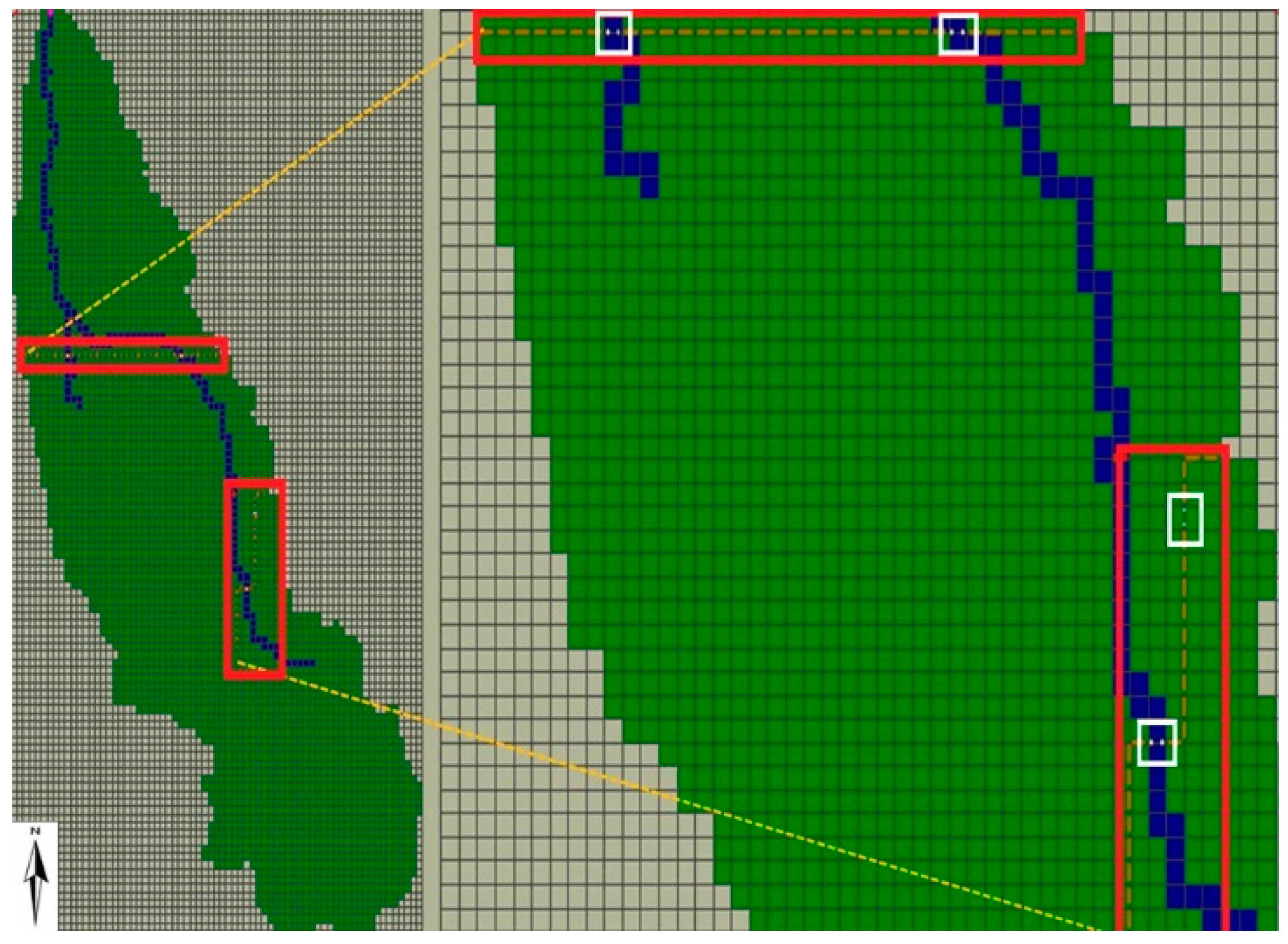
The heterogeneity of the system, such as the vegetation types, soils and topography, can be analyzed through the concept of hydrological response units (HRUs), in which the water balance is quantified on a daily basis, taking into account the spatial variability of the soil type, land use, and topographic slope [119]. A disadvantage when analyzing the water balance at a semi-distributed scale is that they are not connected units but simply a union of cells that present discontinuities [120], that is, the HRUs do not have a spatial continuity [121]. Therefore, it is necessary to make certain assumptions when relating all of them, for example for the groundwater analysis, because HRUs do not take into account distributed parameters such as the hydraulic conductivity and storage coefficient. The SWAT model is particularly limited in terms of dealing with groundwater flow, due to its semi-distributed internal nature. Future research should consider coupling hydrologic and hydrogeologic models to better account for the interactions between surface water and groundwater in plain areas, in order to adequately quantify the spatial and temporal variations in the phreatic level and their influence on the water extremes [86]. Another modelling assumption is that SWAT directly simulates only the saturated flow, and it assumes that water is uniformly distributed within a given layer. Unsaturated flow between layers is indirectly modeled using depth distribution functions for plant water uptake and soil water evaporation [122]. With that being said, we are aware that the more assumptions are made, the weaker the prediction. However, we understand that due to the nature of modelling, which implies a simplification of real-world processes, our results (like any other model results) bear uncertainties. To amend this situation, we quantified many uncertainties so the reader could have an idea of their magnitude.

The integration of SWAT with CTSS8 allowed us to identify changes in water flows, runoff volumes and peak flow characteristics between the baseline scenario and each of the tested hypothetical scenarios. It also enabled us to assess the benefits associated with the implementation of an eco-efficient infrastructure. This combined tool that integrates the use of green infrastructure with the use hydraulic structures could be of great help for territorial planning, allowing one to define flood plains, direct restoration efforts [123] or analyze different scenarios for flood control in plain areas.

The SWAT model let us assess the differences in the surface runoff and soil humidity for each of the assayed scenarios, accounting for the role of green infrastructure associated with land use change [77], including the implantation of riparian forests [124] and the implementation of best management practices in agriculture [125,126]. This represents an approach with potential applications in this or other plain areas, being effective, economically sound and beneficial for the security and wellbeing of populations exposed to water extreme events. Proper management strategies like the above-mentioned ones could help control soil moisture, as pointed out by [127] and could help improve the yields of rainfed-crops.

SWAT allows the assessment of the role of the vegetation cover constituted by forests during water extremes. As seen in the simulations, forests act as regulatory elements of surface hydrological processes [128] because the hydrologic response of basins located in plain areas depends to a great extent on the state of the vegetation cover along with the soil water content.

This study demonstrates how data obtained from satellite images can be integrated into hydrologic-hydraulic modelling in plain areas that are typically associated with surface water accumulation. This methodology allows for a more accurate determination of the flooding surface area and its boundaries, which is particularly important in the absence of flow rate values, as was also suggested by [129,130]. Advances in satellite observation provide important information on various aspects of the storage and movement of surface water, such as the extent of inundated areas, water surface elevation, water depth and river discharge, and variations in terrestrial water storage [131]. As an example of using satellite images for model calibration and validation, [132] satisfactorily used remote sensing data to calibrate and evaluate a coupled hydrologic-hydraulic model of the Zambezi River (Mozambique). Likewise, [133] calibrated a hydraulic model using remotely sensed flood extents, and used this information to update the hydrologically modeled soil moisture values.

Regarding the economic assessment of the impacts of water extremes, as mentioned before, SWAT has the option of performing this assessment. However, CTSS8 does not have a subroutine for calculating the crop biomass, which is required for a crop yield estimation. We believe that future upgrades of CTSS8 should consider including it.

Although reservoirs are common structural measures for flood control, we did not consider one here, since we examined low cost structural measures that would help minimize water extreme effects. In addition, we intended to manage the water on site (i.e., where rain falls) to regulate the runoff and soil moisture, in order to improve the crop yields (or minimize losses). In fact, having a reservoir in a plain area like the one studied here (< 1% slope) is unsuitable because it would imply: (1) massive flooding of large land areas and that (2) dams would need to be considerable long (and expensive to construct) due to the topography that characterizes the region.

It would have been useful to study the changes in sedimentation associated with the implementation of the different hypothetical soil conservation measures and structures in the field, for example to prevent the siltation of specific areas [134]. By modelling this variable and knowing how it behaves under different scenarios, better informed decisions on control measures and management policies could be made to prevent the aggradation phenomenon upstream of hydraulic structures, among others [135]. The same would apply for nutrients and other waterborne compounds. Unfortunately, at the time, there is no such data available for the studied basin, but future research should include these variables as further important model components.

Our study results contribute, with science-based political decision making, in selecting the most suited mitigation practices, taking into account novel approaches such as the use of an eco-efficient infrastructure to control water extremes. This approach favors a decrease of the economic investment in mitigation practices as well as an improvement of the wellbeing of those living and carrying out their productive activities in plain areas like the Pampas region of Argentina.

6. Conclusions

The proposed modelling methodology developed for basins located in plain areas allows for the quantification of the variation of water extremes by integrating hydrologic and hydraulic models. Following a continuous modelling approach using SWAT for the 2006–2012 period, we were able to simulate water extremes for the SCSB under different land use and crop management practice scenarios. The hypothetical increase in the forested riparian strip, the forestation of the deflation hollows and the implementation of contour sowing for crops caused a 28% drop in surface runoff, whereas soil moisture increased by 10% on a daily average for the studied period. This translates into a reduction of the impact of floods and an increase in water availability in the soil during dry periods.

As for the event-based modelling performed with CTSS8, there was a noticeable reduction in peak flows both in volume and in duration. The implementation of hydraulic structures such as embankments and culverts seemed to regulate and reduce the impact of the studied flood by 9%. With the green infrastructure scenario, a 13% decrease in the flood impact was achieved. When joint measures involving the implementation of a green infrastructure and hydraulic structures were modelled, the flood impact was reduced by 21%.

The results of the present study showed that implementing an eco-efficient infrastructure contributes to the effective management of water resources as well as to the improvement of yields for rainfed crops, the latter representing a major economic input for the study region.

However, key points to be considered in future research related to modelling complex natural phenomena include the reduction of uncertainties and the improvement of our assumptions associated with the simplification of the modelled processes. It would also be useful if event-based models were furnished with subroutines for estimating the crop yield (as SWAT is). This would be especially useful in decision-making.

A key contribution of this study is that the integrated use of event-based and continuous models allows for the testing of different hypothetical management strategies before implementing any in the field. Identifying the most suitable strategy would mean that the mitigation of the extreme event would be more effective, diminishing its socio-economic impact.

References

1. Houser, T.; Hsiang, S.; Kopp, R.; Larsen, K. Economic Risks of Climate Change: An American Prospectus; Columbia University Press: New York, NY, USA, 2015; pp. 1–351. [Google Scholar]
2. Zhang, Q.; Gu, X.; Singh, V.P.; Kong, D.; Chen, X. Spatio temporal behavior of floods and droughts and their impacts on agriculture in China. Glob. Planet. Chang. 2015, 131, 63–72. [Google Scholar] [CrossRef]
3. Hanel, M.; Rakovec, O.; Markonis, Y.; Máca, P.; Samaniego, L.; Kyselý, J.; Kumar, R. Revisiting the recent European droughts from a long-term perspective. Sci. Rep. 2018, 8, 1–11. [Google Scholar] [CrossRef] [PubMed]
4. Kron, W. Flood risk = hazard values vulnerability. Water Int. 2005, 30, 58–68. [Google Scholar] [CrossRef]
5. Trenberth, K.E.; Fasullo, J.T.; Shepherd, T.G. Attribution of climate extreme events. Nat. Clim. Chang. 2015, 5, 725–730. [Google Scholar] [CrossRef]
6. Winsemius, H.C.; Aerts, J.C.; van Beek, L.P.; Bierkens, M.F.; Bouwman, A.; Jongman, B.; Ward, P.J. Global drivers of future river flood risk. Nat. Clim. Chang. 2016, 6, 381–385. [Google Scholar] [CrossRef]
7. Leigh, C.; Bush, A.; Harrison, E.T.; Ho, S.S.; Luke, L.; Rolls, R.J.; Ledger, M.E. Ecological effects of extreme climatic events on riverine ecosystems: Insights from Australia. Freshw. Biol. 2015, 60, 2620–2638. [Google Scholar] [CrossRef]
8. Nguyen, L.T.; Osanai, Y.; Anderson, I.C.; Bange, M.P.; Tissue, D.T.; Singh, B.K. Flooding and prolonged drought have differential legacy impacts on soil nitrogen cycling, microbial communities and plant productivity. Plant Soil 2018, 1–17. [Google Scholar] [CrossRef]
9. Bakker, E.S.; Hilt, S. Impact of water-level fluctuations on cyanobacterial blooms: Options for management. Aquat. Ecol. 2016, 50, 485–498. [Google Scholar] [CrossRef]
10. Reich, P.; Lake, P.S. Extreme hydrological events and the ecological restoration of flowing waters. Freshw. Biol. 2015, 60, 2639–2652. [Google Scholar] [CrossRef]
11. Lesk, C.; Rowhani, P.; Ramankutty, N. Influence of extreme weather disasters on global crop production. Nature 2016, 529, 84–87. [Google Scholar] [CrossRef] [PubMed]
12. Chen, H.; Liang, Z.; Liu, Y.; Jiang, Q.; Xie, S. Effects of drought and flood on crop production in China across 1949–2015: Spatial heterogeneity analysis with Bayesian hierarchical modeling. Nat. Hazards 2018, 92, 525–541. [Google Scholar] [CrossRef]
13. Ebi, K.L.; Bowen, K. Extreme events as sources of health vulnerability: Drought as an example. Weather Clim. Extrem. 2016, 11, 95–102. [Google Scholar] [CrossRef] [Green Version]
14. De Silva, M.M.G.T.; Kawasaki, A. Socioeconomic Vulnerability to Disaster Risk: A Case Study of Flood and Drought Impact in a Rural Sri Lankan Community. Ecol. Econ. 2018, 152, 131–140. [Google Scholar] [CrossRef]
15. Quesada-Montano, B.; Di Baldassarre, G.; Rangecroft, S.; Van Loon, A.F. Hydrological change: Towards a consistent approach to assess changes on both floods and droughts. Adv. Water Resour. 2018, 111, 31–35. [Google Scholar] [CrossRef]
16. Stocker, T.F.; Qin, D.; Plattner, G.K.; Tignor, M.; Allen, S.K.; Boschung, J.; Midgley, B.M. IPCC, 2013: Climate change 2013: The physical science basis. In Contribution of Working Group I to the Fifth Assessment Report of the Intergovernmental Panel on Climate Change; IPCC: Geneva, Switzerland, 2013; pp. 1–1535. ISBN 978-1-107-05799-1. [Google Scholar]
17. Hurlbert, M.; Gupta, J. Adaptive governance, uncertainty, and risk: Policy framing and responses to climate change, drought, and flood. Risk Anal. 2016, 36, 339–356. [Google Scholar] [CrossRef] [PubMed]
18. Vogel, R.M.; Lall, U.; Cai, X.; Rajagopalan, B.; Weiskel, P.K.; Hooper, R.P.; Matalas, N.C. Hydrology: The interdisciplinary science of water. Water Resour. Res. 2015, 51, 4409–4430. [Google Scholar] [CrossRef]
19. Güneralp, B.; Güneralp, İ.; Liu, Y. Changing global patterns of urban exposure to flood and drought hazards. Glob. Environ. Chang. 2015, 31, 217–225. [Google Scholar] [CrossRef]
20. Welle, T.; Birkmann, J. The world risk index–an approach to assess risk and vulnerability on a global scale. J. Extrem. Events 2015, 2, 1550003. [Google Scholar] [CrossRef]
21. Johnston, A.M.; Tanaka, D.L.; Miller, P.R.; Brandt, S.A.; Nielsen, D.C.; Lafond, G.P.; Riveland, N.R. Oilseed crops for semiarid cropping systems in the northern Great Plains. Agron. J. 2002, 94, 231–240. [Google Scholar] [CrossRef]
22. Cotterman, K.A.; Kendall, A.D.; Basso, B.; Hyndman, D.W. Groundwater depletion and climate change: Future prospects of crop production in the Central High Plains Aquifer. Clim. Chang. 2018, 146, 187–200. [Google Scholar] [CrossRef]
23. Hu, H.; Lu, C.; Wang, Q.; Li, H.; He, J.; Xu, D.; Wang, X. Influences of wide-narrow seeding on soil properties and winter wheat yields under conservation tillage in North China Plain. Int. J. Agric. Biol. Eng. 2018, 11, 74–80. [Google Scholar] [CrossRef]
24. Wienhold, B.J.; Vigil, M.F.; Hendrickson, J.R.; Derner, J.D. Vulnerability of crops and croplands in the US Northern Plains to predicted climate change. Clim. Chang. 2018, 146, 219–230. [Google Scholar] [CrossRef]
25. Rockström, J.; Karlberg, L.; Wani, S.P.; Barron, J.; Hatibu, N.; Oweis, T.; Qiang, Z. Managing water in rainfed agriculture-The need for a paradigm shift. Agric. Water Manag. 2010, 97, 543–550. [Google Scholar] [CrossRef]
26. Rao, C.S.; Gopinath, K.A.; Rao, C.R.; Raju, B.M.K.; Rejani, R.; Venkatesh, G.; Kumari, V.V. Dryland agriculture in South Asia: Experiences, challenges and opportunities. In Innovations in Dryland Agriculture; Springer: Cham, Switzerland, 2016; pp. 345–392. [Google Scholar]
27. Nath, R.; Nath, D.; Li, Q.; Chen, W.; Cui, X. Impact of drought on agriculture in the Indo-Gangetic Plain, India. Adv. Atmos. Sci. 2017, 34, 335–346. [Google Scholar] [CrossRef]
28. Qin, W.; Wang, D.; Guo, X.; Yang, T.; Oenema, O. Productivity and sustainability of rainfed wheat-soybean system in the North China Plain: Results from a long-term experiment and crop modelling. Sci. Rep. 2015, 5, 17514. [Google Scholar] [CrossRef] [PubMed]
29. Matteucci, S.D.; Rodriguez, A.; Silva, M. Ecorregiones y Complejos Ecosistémicos Argentinos; Orientación Gráfica Editora: Buenos Aires, Argentina, 2012; pp. 391–436. [Google Scholar]
30. Viglizzo, E.F.; Jobbágy, E.G.; Carreño, L.; Frank, F.C.; Aragón, R.; Oro, L.D.; Salvador, V. The dynamics of cultivation and floods in arable lands of Central Argentina. Hydrol. Earth Syst. Sci. 2009, 13, 491–502. [Google Scholar] [CrossRef] [Green Version]
31. Aragón, R.; Jobbágy, E.G.; Viglizzo, E.F. Surface and groundwater dynamics in the sedimentary plains of the Western Pampas (Argentina). Ecohydrology 2011, 4, 433–447. [Google Scholar] [CrossRef]
32. Scarpati, O.E.; Capriolo, A.D. Droughts and floods in Buenos Aires province (Argentina) and their space and temporal distribution. Investig. Geogr. Boletín Inst. Geogr. 2013, 82, 38–51. [Google Scholar]
33. Latrubesse, E.M.; Brea, D. Floods in Argentina. Dev. Earth Surf. Process. 2009, 13, 333–349. [Google Scholar] [CrossRef]
34. Garner, G.; Van Loon, A.F.; Prudhomme, C.; Hannah, D.M. Hydroclimatology of extreme river flows. Freshw. Biol. 2015, 60, 2461–2476. [Google Scholar] [CrossRef]
35. Narasimhan, B.; Srinivasan, R.; Arnold, J.G.; Di Luzio, M. Estimation of long-term soil moisture using a distributed parameter hydrologic model and verification using remotely sensed data. Trans. ASABE 2005, 48, 1101–1113. [Google Scholar] [CrossRef]
36. Jain, V.K.; Pandey, R.P.; Jain, M.K. Spatio-temporal assessment of vulnerability to drought. Nat. Hazards 2015, 76, 443–469. [Google Scholar] [CrossRef]
37. Mercau, J.L.; Nosetto, M.D.; Bert, F.; Giménez, R.; Jobbágy, E.G. Shallow groundwater dynamics in the Pampas: Climate, landscape and crop choice effects. Agric. Water Manag. 2016, 163, 159–168. [Google Scholar] [CrossRef]
38. Kuppel, S.; Houspanossian, J.; Nosetto, M.D.; Jobbágy, E.G. What does it take to flood the Pampas?: Lessons from a decade of strong hydrological fluctuations. Water Resour. Res. 2015, 51, 2937–2950. [Google Scholar] [CrossRef]
39. Wang, Z.; Ma, Q.; Chen, S.; Deng, L.; Jiang, J. Empirical study on drought adaptation of regional rainfed agriculture in China. Nat. Hazards Earth Syst. Sci. 2016, 3, 1–29. [Google Scholar] [CrossRef]
40. Tucci, C.E. Urban Flood Management; World Meteorological Organization and International Network for Capacity Building in Integrated Water Resources Management: Porto Alegre, Brazil, 2007; pp. 1–303. [Google Scholar]
41. Beilinson, E.; Gasparini, G.M.; Soibelzon, L.H.; Soibelzon, E. Insights into Pleistocene palaeoenvironments and biostratigraphy in southern Buenos Aires province (Argentina) from continental deposits. J. S. Am. Earth Sci. 2015, 60, 82–91. [Google Scholar] [CrossRef]
42. Kruse, E.; Zimmermann, E. Hidrogeología de grandes llanuras: Particularidades en la llanura pampeana (Argentina). In Workshop Publication on Groundwater and Human Development; Consejo Hídrico Federal: Santa Fé, Argentina, 2002; pp. 2025–2038. [Google Scholar]
43. Wilhite, D.A. Drought as a natural hazard: Concepts and definitions. In Droughts: A Global Assessment; Routledge: Abingdon, UK, 2000; pp. 3–18. [Google Scholar]
44. Mishra, A.K.; Singh, V.P. A review of drought concepts. J. Hydrol. 2010, 391, 202–216. [Google Scholar] [CrossRef]
45. Mishra, A.K.; Singh, V.P. Drought modeling—A review. J. Hydrol. 2011, 403, 157–175. [Google Scholar] [CrossRef]
46. Yaseen, Z.M.; Sulaiman, S.O.; Deo, R.C.; Chau, K.W. An enhanced extreme learning machine model for river flow forecasting: State-of-the-art, practical applications in water resource engineering area and future research direction. J. Hydrol. 2018, 569, 387–408. [Google Scholar] [CrossRef]
47. Moazenzadeh, R.; Mohammadi, B.; Shamshirband, S.; Chau, K.W. Coupling a firefly algorithm with support vector regression to predict evaporation in northern Iran. Eng. Appl. Comput. Fluid Mech. 2018, 12, 584–597. [Google Scholar] [CrossRef] [Green Version]
48. Zhang, C.X.; You, X.Y. Application of EFDC model to grading the eutrophic state of reservoir: Case study in Tianjin Erwangzhuang Reservoir, China. Eng. Appl. Comput. Fluid Mech. 2017, 11, 111–126. [Google Scholar] [CrossRef]
49. Gallerano, F.; Cannata, G.; Scarpone, S. Bottom changes in coastal areas with complex shorelines. Eng. Appl. Comput. Fluid Mech. 2017, 11, 396–416. [Google Scholar] [CrossRef]
50. Farhadi, A.; Mayrhofer, A.; Tritthart, M.; Glas, M.; Habersack, H. Accuracy and comparison of standard k-ϵ with two variants of k-ω turbulence models in fluvial applications. Eng. Appl. Comput. Fluid Mech. 2018, 12, 216–235. [Google Scholar] [CrossRef]
51. Chuntian, C.; Chau, K.W. Three-person multi-objective conflict decision in reservoir flood control. Eur. J. Oper. Res. 2002, 142, 625–631. [Google Scholar] [CrossRef] [Green Version]
52. Grimaldi, S.; Schumann, G.P.; Shokri, A.; Walker, J.P.; Pauwels, V.R.N. Challenges, opportunities and pitfalls for global coupled hydrologic-hydraulic modeling of floods. Water Resour. Res. 2019, 1–24. [Google Scholar] [CrossRef]
53. Refsgaard, J.C.; Henriksen, H.J. Modelling guidelines—Terminology and guiding principles. Adv. Water Resour. 2004, 27, 71–82. [Google Scholar] [CrossRef]
54. Chu, X.; Steinman, A. Event and continuous hydrologic modeling with HEC-HMS. J. Irrig. Drain. Eng. 2009, 135, 119–124. [Google Scholar] [CrossRef]
55. Singh, V.P.; Woolhiser, D.A. Mathematical modeling of watershed hydrology. J. Hydrol. Eng. 2002, 7, 270–292. [Google Scholar] [CrossRef]
56. Falter, D.; Schröter, K.; Dung, N.V.; Vorogushyn, S.; Kreibich, H.; Hundecha, Y.; Merz, B. Spatially coherent flood risk assessment based on long-term continuous simulation with a coupled model chain. J. Hydrol. 2015, 524, 182–193. [Google Scholar] [CrossRef]
57. Fatichi, S.; Vivoni, E.R.; Ogden, F.L.; Ivanov, V.Y.; Mirus, B.; Gochis, D.; Jones, N. An overview of current applications, challenges, and future trends in distributed process-based models in hydrology. J. Hydrol. 2016, 537, 45–60. [Google Scholar] [CrossRef] [Green Version]
58. Borah, D.K.; Arnold, J.G.; Bera, M.; Krug, E.C.; Liang, X.Z. Storm event and continuous hydrologic modeling for comprehensive and efficient watershed simulations. J. Hydrol. Eng. 2007, 12, 605–616. [Google Scholar] [CrossRef]
59. Thompson, J.R.; Sørenson, H.R.; Gavin, H.; Refsgaard, A. Application of the coupled MIKE SHE/MIKE 11 modelling system to a lowland wet grassland in southeast England. J. Hydrol. 2004, 293, 151–179. [Google Scholar] [CrossRef]
60. Bravo, J.M.; Allasia, D.; Paz, A.R.; Collischonn, W.; Tucci, C.E.M. Coupled hydrologic-hydraulic modeling of the Upper Paraguay River basin. J. Hydrol. Eng. 2011, 17, 635–646. [Google Scholar] [CrossRef]
61. Tahmasbinejad, H.; Feyzolahpour, M.; Mumipour, M.; Zakerhoseini, F. Rainfall-runoff Simulation and Modeling of Karon River Using HEC-RAS and HEC-HMS Models, Izeh District, Iran. J. Appl. Sci. (Faisalabad) 2012, 12, 1900–1908. [Google Scholar] [CrossRef]
62. Quiroga, V.M.; Popescu, I.A.; Solomatine, D.P.; Bociort, L. Cloud and cluster computing in uncertainty analysis of integrated flood models. J. Hydroinform. 2013, 15, 55–70. [Google Scholar] [CrossRef]
63. Arnold, J.G.; Moriasi, D.N.; Gassman, P.W.; Abbaspour, K.C.; White, M.J.; Srinivasan, R.; Kannan, N. SWAT: Model use, calibration, and validation. Trans. ASABE 2012, 55, 1491–1508. [Google Scholar] [CrossRef]
64. Riccardi, G. A cell model for hydrological-hydraulic modeling. J. Environ. Hydrol. 2000, 8, 1–13. [Google Scholar]
65. Basile, P.A.; Riccardi, G.A.; Zimmermann, E.D.; Stenta, H.R. Simulation of erosion-deposition processes at basin scale by a physically-based mathematical model. Int. J. Sediment Res. 2010, 25, 91–109. [Google Scholar] [CrossRef]
66. Garcia, M.L.; Basile, P.A.; Riccardi, G.A.; Rodriguez, J.F. Modelling extraordinary floods and sedimentological processes in a large channel-floodplain system of the Lower Paraná River (Argentina). Int. J. Sediment Res. 2015, 30, 150–159. [Google Scholar] [CrossRef]
67. Wester, S.J.; Grimson, R.; Minotti, P.G.; Booij, M.J.; Brugnach, M. Hydrodynamic modelling of a tidal delta wetland using an enhanced quasi-2D model. J. Hydrol. 2018, 559, 315–326. [Google Scholar] [CrossRef]
68. Cai, J.; Kummu, M.; Niva, V.; Guillaume, J.H.; Varis, O. Exposure and resilience of China’s cities to floods and droughts: A double-edged sword. Int. J. Water Resour. Dev. 2018, 34, 547–565. [Google Scholar] [CrossRef]
69. Novak, P.; Moffat, A.I.B.; Nalluri, C.; Narayanan, R. Hydraulic Structures; CRC Press: Boca Raton, FL, USA, 2014; pp. 1–696. ISBN 978-041-530608-9. [Google Scholar]
70. Di Baldassarre, G.; Martinez, F.; Kalantari, Z.; Viglione, A. Drought and flood in the Anthropocene: Feedback mechanisms in reservoir operation. Earth Syst. Dyn. 2017, 8, 1–9. [Google Scholar] [CrossRef]
71. Sen, Z. Flood Design Discharge and Case Studies. In Flood Modeling, Prediction and Mitigation; Springer: Cham, Switzerland, 2018; pp. 303–335. [Google Scholar]
72. Posthumus, H.; Hewett, C.J.M.; Morris, J.; Quinn, P.F. Agricultural land use and flood risk management: Engaging with stakeholders in North Yorkshire. Agric. Water Manag. 2008, 95, 787–798. [Google Scholar] [CrossRef]
73. Schuch, G.; Serrao-Neumann, S.; Morgan, E.; Choy, D.L. Water in the city: Green open spaces, land use planning and flood management-An Australian case study. Land Use Policy 2017, 63, 539–550. [Google Scholar] [CrossRef]
74. O’Donnell, E.C.; Lamond, J.E.; Thorne, C.R. Recognising barriers to implementation of Blue-Green Infrastructure: A Newcastle case study. Urban Water J. 2017, 14, 964–971. [Google Scholar] [CrossRef]
75. Shreve, C.M.; Kelman, I. Does mitigation save? Reviewing cost-benefit analyses of disaster risk reduction. Int. J. Disaster Risk Reduct. 2014, 10, 213–235. [Google Scholar] [CrossRef] [Green Version]
76. Roudier, P.; Andersson, J.C.; Donnelly, C.; Feyen, L.; Greuell, W.; Ludwig, F. Projections of future floods and hydrological droughts in Europe under a+ 2 C global warming. Clim. Chang. 2016, 135, 341–355. [Google Scholar] [CrossRef]
77. Barraqué, B. The common property issue in flood control through land use in France. J. Flood Risk Manag. 2017, 10, 182–194. [Google Scholar] [CrossRef]
78. Jang, S.S.; Ahn, S.R.; Kim, S.J. Evaluation of executable best management practices in Haean highland agricultural catchment of South Korea using SWAT. Agric. Water Manag. 2017, 180, 224–234. [Google Scholar] [CrossRef]
79. Mander, Ü.; Tournebize, J.; Tonderski, K.; Verhoeven, J.T.; Mitsch, W.J. Planning and establishment principles for constructed wetlands and riparian buffer zones in agricultural catchments. Ecol. Eng. 2017, 103, 296–300. [Google Scholar] [CrossRef]
80. Larson, D.M.; Dodds, W.K.; Veach, A.M. Removal of Woody Riparian Vegetation Substantially Altered a Stream Ecosystem in an Otherwise Undisturbed Grassland Watershed. Ecosystems 2018, 1–13. [Google Scholar] [CrossRef]
81. McVittie, A.; Norton, L.; Martin-Ortega, J.; Siameti, I.; Glenk, K.; Aalders, I. Operation an ecosystem services-based approach using Bayesian Belief Networks: An application to riparian buffer strips. Ecol. Econ. 2015, 110, 15–27. [Google Scholar] [CrossRef]
82. Kuglerová, L.; Ågren, A.; Jansson, R.; Laudon, H. Towards optimizing riparian buffer zones: Ecological and biogeochemical implications for forest management. For. Ecol. Manag. 2014, 334, 74–84. [Google Scholar] [CrossRef]
83. Tiwari, T.; Lundström, J.; Kuglerová, L.; Laudon, H.; Öhman, K.; Ågren, A.M. Cost of riparian buffer zones: A comparison of hydrologically adapted site-specific riparian buffers with traditional fixed widths. Water Resour. Res. 2016, 52, 1056–1069. [Google Scholar] [CrossRef] [Green Version]
84. Hille, S.; Andersen, D.K.; Kronvang, B.; Baattrup-Pedersen, A. Structural and functional characteristics of buffer strip vegetation in an agricultural landscape-high potential for nutrient removal but low potential for plant biodiversity. Sci. Total Environ. 2018, 628, 805–814. [Google Scholar] [CrossRef] [PubMed]
85. Guevara-Ochoa, C.; Briceño, N.; Zimmermann, E.; Vives, L.; Blanco, M.; Cazenave, G.; Ares, G. Filling series of daily precipitation for long periods of time in plain areas. case study superior basin of stream del Azul. Geoacta 2017, 42, 38–62. [Google Scholar]
86. Guevara-Ochoa, C. Una Metodología Para el Análisis de los Patrones Espacio Temporales de la Interacción Entre Aguas Superficiales y Subterráneas en Areas de Llanura bajo Escenarios de Cambio Climático. Ph.D. Thesis, Facultad de Ingeniería, Universidad Nacional de Rosario, Rosario, Argentina, 2019; pp. 1–178. [Google Scholar]
87. Zárate, M.; Mehl, A. Geología y geomorfología de la cuenca del Arroyo del Azul, provincia de Buenos Aires, Argentina. En: I Congreso Internacional de Hidrología de Llanuras. Hacia Gest. Integral Recur. Hídricos Zonas Llanura 2010, 1, 65–78. [Google Scholar]
88. Silva, A.A.; Amato, S.D. Aspectos hidrogeológicos de la región periserrana de Tandilia (Buenos Aires, Argentina). Boletín Geol. Min. 2012, 123, 27–40. [Google Scholar]
89. McKee, T.B.; Doesken, N.J.; Kleist, J. The relationship of drought frequency and duration to time scales. In Preprints. In Proceedings of the 8th Conference on Applied Climatology, Anaheim, CA, USA, 17–22 January 1993; pp. 179–184. [Google Scholar]
90. World Meteorological Organization. Índice Normalizado de Precipitación, Guía del Usuario; World Meteorological Organization: Geneva, Switzerland, 2012; Volume 1090, pp. 1–16. ISBN 978-92-63-31090-3. [Google Scholar]
91. Rivera, J.A.; Penalba, O.C. Trends and spatial patterns of drought affected area in Southern South America. Climate 2014, 2, 264–278. [Google Scholar] [CrossRef]
92. Viglizzo, E.F.; Roberto, Z.E.; Filippin, M.C.; Pordomingo, A.J. Climate variability and agroecological change in the Central Pampas of Argentina. Agric. Ecosyst. Environ. 1995, 55, 7–16. [Google Scholar] [CrossRef]
93. Barros, V.R.; Doyle, M.E.; Camilloni, I.A. Precipitation trends in southeastern South America: Relationship with ENSO phases and with low-level circulation. Theor. Appl. Climatol. 2008, 93, 19–33. [Google Scholar] [CrossRef]
94. Barros, V.R.; Boninsegna, J.A.; Camilloni, I.A.; Chidiak, M.; Magrín, G.O.; Rusticucci, M. Climate change in Argentina: Trends, projections, impacts and adaptation. Wiley Interdiscip. Rev. Clim. Chang. 2015, 6, 151–169. [Google Scholar] [CrossRef]
95. Minetti, J.L.; Vargas, W.M. Trends and jumps in the annual precipitation in South America, south of the 15 S. Atmósfera 2009, 11, 205–221. [Google Scholar]
96. Antico, P.L.; Sabbione, N.C. Variabilidad temporal de la precipitación en la ciudad de La Plata durante el período 1909–2007: Tendencia y fluctuaciones cuasiperiódicas. Geoacta 2010, 35, 44–53. [Google Scholar]
97. Maenza, R.A.; Agosta, E.A.; Bettolli, M.L. Climate change and precipitation variability over the western ‘Pampas’ in Argentina. Int. J. Climatol. 2017, 37, 445–463. [Google Scholar] [CrossRef]
98. Jayakrishnan, R.S.R.S.; Srinivasan, R.; Santhi, C.; Arnold, J.G. Advances in the application of the SWAT model for water resources management. Hydrol. Process. 2005, 19, 749–762. [Google Scholar] [CrossRef]
99. Neitsch, S.L.; Williams, J.R.; Arnold, J.G.; Kiniry, J.R. Soil and Water Assessment Tool Theoretical Documentation Version 2009; Texas Water Resources Institute: College Station, TX, USA, 2011. [Google Scholar]
100. SCS. Urban hydrology for small watersheds. US Soil Conservation Service. Tech. Release 1986, 55, 13. [Google Scholar]
101. Shao, G.; Zhang, D.; Guan, Y.; Xie, Y.; Huang, F. Application of SWAT Model with a Modified Groundwater Module to the Semi-Arid Hailiutu River Catchment, Northwest China. Sustainability 2019, 11, 2031. [Google Scholar] [CrossRef]
102. Riccardi, G.; Stenta, H.; Scuderi, C.; Basile, P.; Zimmermann, E.; Trivisonno, F. Aplicación de un modelo hidrológico-hidráulico para el pronóstico de niveles de agua en tiempo real. Tecnol. Cienc. Agua 2013, 4, 83–105. [Google Scholar]
103. Amlin, N.A.; Rood, S.B. Inundation tolerances of riparian willows and cottonwoods. J. Am. Water Resour. Assoc. 2001, 37, 1709–1720. [Google Scholar] [CrossRef]
104. Yang, J.; Zhao, H.; Zhang, T. Heat and drought tolerance of two willow species, Salix gordejevii and Salix babylonica: A comparative study. Isr. J. Plant Sci. 2004, 52, 301–306. [Google Scholar] [CrossRef]
105. INTA. Cartas de Suelos, 1:50000; Publicaciones del Instituto Nacional de Tecnología Agropecuaria de Argentina (INTA): Buenos Aires, Argentina, 1992. [Google Scholar]
106. Entraigas, I. Implementación de Sistemas de Soporte de Decisiones Multipropósito a Escalas Urbana y Rural. Ph.D. Thesis, Facultad de Ciencias Naturales Y Museo, Universidad Nacional de la Plata, La Plata, Argentina, 2008; pp. 90–100. [Google Scholar]
107. Arnold, J.G.; Kiniry, J.R.; Srinivasan, R.; Williams, J.R.; Haney, E.B.; Neitsch, S.L. SWAT 2012 Input/Output Documentation; Texas Water Resources Institute: College Station, TX, USA, 2013. [Google Scholar]
108. Rabus, B.; Eineder, M.; Roth, A.; Bamler, R. The shuttle radar topography mission-a new class of digital elevation models acquired by spaceborne radar. ISPRS J. Photogramm. Remote Sens. 2003, 57, 241–262. [Google Scholar] [CrossRef]
109. Gesch, D.B.; Muller, J.; Farr, T.G. The Shuttle Radar Topography Mission-Data Validation and Applications. Photogramm. Eng. Remote Sens. 2006, 72, 233–237. [Google Scholar]
110. Guevara-Ochoa, C.; Vives, L.; Zimmermann, E.; Masson, I.; Fajardo, L.; Scioli, C. Analysis and Correction of Digital Elevation Models for Plain Areas. Photogramm. Eng. Remote Sens. 2019, 85, 209–219. [Google Scholar] [CrossRef]
111. Abbaspour, K.C. User Manual for SWAT-CUP, SWAT Calibration and Uncertainty Analysis Program; Swiss Federal Institute of Aquatic Science and Technology, Eawag: Dübendorf, Switzerland, 2007; pp. 1–93. [Google Scholar]
112. Moriasi, D.N.; Arnold, J.G.; Van Liew, M.W.; Bingner, R.L.; Harmel, R.D.; Veith, T.L. Model evaluation guidelines for systematic quantification of accuracy in watershed simulations. Trans. ASABE 2007, 50, 885–900. [Google Scholar] [CrossRef]
113. Krause, P.; Boyle, D.P.; Bäse, F. Comparison of different efficiency criteria for hydrological model assessment. Adv. Geosci. 2005, 5, 89–97. [Google Scholar] [CrossRef] [Green Version]
114. Tapley, B.D.; Bettadpur, S.; Ries, J.C.; Thompson, P.F.; Watkins, M.M. GRACE measurements of mass variability in the Earth system. Science 2004, 305, 503–505. [Google Scholar] [CrossRef] [PubMed]
115. Wouters, B.; Bonin, J.A.; Chambers, D.P.; Riva, R.E.M.; Sasgen, I.; Wahr, J. GRACE, time-varying gravity, Earth system dynamics and climate change. Rep. Prog. Phys. 2014, 77, 1–41. [Google Scholar] [CrossRef] [PubMed]
116. Maxwell, R.M.; Chow, F.K.; Kollet, S.J. The groundwater–land-surface–atmosphere connection: Soil moisture effects on the atmospheric boundary layer in fully-coupled simulations. Adv. Water Resour. 2007, 30, 2447–2466. [Google Scholar] [CrossRef]
117. Poméon, T.; Diekkrüger, B.; Springer, A.; Kusche, J.; Eicker, A. Multi-Objective Validation of SWAT for Sparsely-Gauged West African River Basins—A Remote Sensing Approach. Water 2018, 10, 451. [Google Scholar] [CrossRef]
118. Trambauer, P.; Maskey, S.; Winsemius, H.; Werner, M.; Uhlenbrook, S. A review of continental scale hydrological models and their suitability for drought forecasting in (sub-Saharan) Africa. Phys. Chem. Earth Parts A B C 2013, 66, 16–26. [Google Scholar] [CrossRef]
119. Kim, N.W.; Chung, I.M.; Won, Y.S.; Arnold, J.G. Development and application of the integrated SWAT–MODFLOW model. J. Hydrol. 2008, 356, 1–16. [Google Scholar] [CrossRef]
120. Olaya, V. Hidrología Computacional y Modelos Digitales del Terreno-Teoría, Práctica y Filosofía de una Nueva Forma de Análisis Hidrológico; V. Olaya Editora: Madrid, Spain, 2004; pp. 1–391. [Google Scholar]
121. Guzman, J.A.; Moriasi, D.N.; Gowda, P.H.; Steiner, J.L.; Starks, P.J.; Arnold, J.G.; Srinivasan, R. A model integration framework for linking SWAT and MODFLOW. Environ. Model. Softw. 2015, 73, 103–116. [Google Scholar] [CrossRef]
122. Narasimhan, B.; Srinivasan, R. Development and evaluation of Soil Moisture Deficit Index (SMDI) and Evapotranspiration Deficit Index (ETDI) for agricultural drought monitoring. Agric. For. Meteorol. 2005, 133, 69–88. [Google Scholar] [CrossRef]
123. Tockner, K.; Stanford, J.A. Riverine flood plains: Present state and future trends. Environ. Conserv. 2002, 29, 308–330. [Google Scholar] [CrossRef]
124. Luke, S.H.; Slade, E.M.; Gray, C.L.; Annammala, K.V.; Drewer, J.; Williamson, J.; Struebig, M.J. Riparian buffers in tropical agriculture: Scientific support, effectiveness, and directions for policy. J. Appl. Ecol. 2018. [Google Scholar] [CrossRef]
125. Howden, S.M.; Soussana, J.F.; Tubiello, F.N.; Chhetri, N.; Dunlop, M.; Meinke, H. Adapting agriculture to climate change. Proc. Natl. Acad. Sci. USA 2007, 104, 19691–19696. [Google Scholar] [CrossRef] [PubMed] [Green Version]
126. Kosmowski, F. Soil water management practices (terraces) helped to mitigate the 2015 drought in Ethiopia. Agric. Water Manag. 2018, 204, 11–16. [Google Scholar] [CrossRef] [PubMed]
127. Laio, F.; Porporato, A.; Ridolfi, L.; Rodriguez-Iturbe, I. Plants in water-controlled ecosystems: Active role in hydrologic processes and response to water stress: II. Probabilistic soil moisture dynamics. Adv. Water Resour. 2001, 24, 707–723. [Google Scholar] [CrossRef]
128. Sun, G.; Zhou, G.; Zhang, Z.; Wei, X.; McNulty, S.G.; Vose, J.M. Potential water yield reduction due to forestation across China. J. Hydrol. 2006, 328, 548–558. [Google Scholar] [CrossRef]
129. Sun, W.; Fan, J.; Wang, G.; Ishidaira, H.; Bastola, S.; Yu, J.; Xu, Z. Calibrating a hydrological model in a regional river of the Qinghai–Tibet plateau using river water width determined from high spatial resolution satellite images. Remote Sens. Environ. 2018, 214, 100–114. [Google Scholar] [CrossRef]
130. Hostache, R.; Chini, M.; Giustarini, L.; Neal, J.; Kavetski, D.; Wood, M.; Matgen, P. Near-Real-Time Assimilation of SAR-Derived Flood Maps for Improving Flood Forecasts. Water Resour. Res. 2018, 54, 5516–5535. [Google Scholar] [CrossRef]
131. Yamazaki, D.; Kanae, S.; Kim, H.; Oki, T. A physically based description of floodplain inundation dynamics in a global river routing model. Water Resour. Res. 2011, 47. [Google Scholar] [CrossRef]
132. Schumann, G.P.; Neal, J.C.; Voisin, N.; Andreadis, K.M.; Pappenberger, F.; Phanthuwongpakdee, N.; Bates, P.D. A first large-scale flood inundation forecasting model. Water Resour. Res. 2013, 49, 6248–6257. [Google Scholar] [CrossRef]
133. Montanari, M.; Hostache, R.; Matgen, P.; Schumann, G.; Pfister, L.; Hoffmann, L. Calibration and sequential updating of a coupled hydrologic-hydraulic model using remote sensing-derived water stages. Hydrol. Earth Syst. Sci. 2009, 13, 367–380. [Google Scholar] [CrossRef] [Green Version]
134. Molino, B.; Viparelli, R.; De Vincenzo, A. Effects of river network works and soil conservation measures on reservoir siltation. Int. J. Sediment Res. 2007, 22, 273–281. [Google Scholar]
135. De Vincenzo, A.; Covelli, C.; Molino, A.; Pannone, M.; Ciccaglione, M.; Molino, B. Long-Term Management Policies of Reservoirs: Possible Re-Use of Dredged Sediments for Coastal Nourishment. Water 2019, 11, 15. [Google Scholar] [CrossRef]
Figure 1. Study area: Santa Catalina stream basin.
Hydrology 06 00070 g001
Figure 2. Left: Satellite Pour l’Observation de la Terre (SPOT) satellite image of the Santa Catalina stream basin (and magnification of the lower part of the basin) during a period of water excess (9/13/2012). The Santa Catalina stream watercourse is shown in blue. The encircled area shows the connected deflation hollows running parallel to the stream course. Right: Aerial photographs showing the connection among the water-impounded deflation hollows.
Hydrology 06 00070 g002
Figure 3. Twelve-month SPI for the Santa Catalina stream basin from 1901 to 2015.
Hydrology 06 00070 g003
Figure 4. Methodological flow chart.
Hydrology 06 00070 g004
Figure 5. Map of the land use change scenario (SWT1) for the Santa Catalina stream basin used for the SWAT simulation.
Hydrology 06 00070 g005
Figure 6. Location of hydraulic structures in the Santa Catalina stream basin. Embankments (brown lines) and culverts (white polygons). The basin area and stream course are in green and blue, respectively.
Hydrology 06 00070 g006
Figure 7. Santa Catalina stream basin maps: (a) soil types; (b) land uses; and (c) digital elevation model (DEM).
Hydrology 06 00070 g007
Figure 8. Results of the sensitivity analysis performed on the SWAT model parameters for the Santa Catalina Basin.
Hydrology 06 00070 g008
Figure 9. Santa Catalina stream basin daily streamflow and precipitation for the calibration and validation periods. Observed streamflow (red), simulated streamflow (blue), observed precipitation (black).
Hydrology 06 00070 g009
Figure 10. Monthly changes in the estimated water storage for the Santa Catalina stream basin as calculated from the GRACE images (red) and as modelled with SWAT (blue).
Hydrology 06 00070 g010
Figure 11. The CTSS8 hydrograph for the 08/19/2002 precipitation event. Observed (red) and simulated (blue).
Hydrology 06 00070 g011
Figure 12. Santa Catalina stream basin map showing the concordance between the simulated (CTSS8 model) and the observed (SPOT image) water impounded areas for the event registered on 05/17/2012. The SPOT image was taken on 05/18/2012. The blue pixels indicate a concordance, whereas the red pixels depict a lack of concordance.
Hydrology 06 00070 g012
Figure 13. (top) Annual and (bottom) monthly water balances for the Santa Catalina stream basin. Precipitation (PCP, blue), percolation (PERC, orange), soil moisture (SW, green), surface runoff (SURQ, black) and evapotranspiration (ET, gray), as simulated with SWAT for the 2006–2012 period.
Hydrology 06 00070 g013
Figure 14. The Santa Catalina stream basin crops yields for the 2003–2013 period. Winter wheat (blue) and soybean (green).
Hydrology 06 00070 g014
Figure 15. The daily surface runoff for the Santa Catalina stream basin for the 2006–2012 period under three different scenarios: baseline scenario (blue), SWT1 “land use change” scenario (yellow), and SWT2 “land use change combined with contour farming” scenario (black).
Hydrology 06 00070 g015
Figure 16. Daily soil moisture for the Santa Catalina stream basin for the 2006–2012 period under three different scenarios: baseline scenario (blue), SWT1 scenario (yellow), and SWT2 scenario (black).
Hydrology 06 00070 g016
Figure 17. The hydrographs for the studied scenarios as modeled with CTSS8. Baseline scenario (blue), CTS1 scenario (yellow), CTS2 scenario (green), and CTS3 scenario (red).
Hydrology 06 00070 g017