Article

Evidence for Pathways of Concentrated Submarine Groundwater Discharge in East Antarctica from Helicopter-Borne Electrical Resistivity Measurements

1
Department of Earth and Planetary Sciences, University of California, Santa Cruz, CA 95061, USA
2
Department of Geoscience, Aarhus University, Aarhus, 8000 Midtjylland, Denmark
3
Geology and Geophysics, Louisiana State University, Baton Rouge, LA 70803, USA
4
Department of Microbiology, University of Tennessee, Knoxville, TN 37996, USA
5
Center for Limnology, University of Wisconsin - Madison, Madison, WI 53706, USA
6
Environmental Studies Program, Dartmouth College, Hanover, NH 03755, USA
*
Author to whom correspondence should be addressed.
Hydrology 2019, 6(2), 54; https://doi.org/10.3390/hydrology6020054
Submission received: 12 March 2019 / Revised: 12 June 2019 / Accepted: 16 June 2019 / Published: 20 June 2019
(This article belongs to the Special Issue Submarine Groundwater Discharge and Its Effects)

Abstract

:
The Southern Ocean receives limited liquid surface water input from the Antarctic continent. It has been speculated, however, that significant liquid water may flow from beneath the Antarctic Ice Sheet, and that this subglacial flow carries that water along with dissolved nutrients to the coast. The delivery of solutes, particularly limiting nutrients like bioavailable iron, to the Southern Ocean may contribute to ecosystem processes including primary productivity. Using a helicopter-borne time domain electromagnetic survey along the coastal margins of the McMurdo Dry Valleys region of Southern Victoria Land, Antarctica, we detected subsurface connections between inland lakes, aquifers, and subglacial waters. These waters, which appear as electrically conductive anomalies, are saline and may contain high concentrations of biologically important ions, including iron and silica. Local hydraulic gradients may drive these waters to the coast, where we postulate they emerge as submarine groundwater discharge. This high latitude groundwater system, imaged regionally in the McMurdo Dry Valleys, may be representative of a broader system of Antarctic submarine groundwater discharge that fertilizes the Southern Ocean. In total, it has the potential to deliver tens of gigagrams of bioavailable Fe and Si to the coastal zone.

1. Introduction

Submarine Groundwater Discharge (SGD) is broadly defined as the flow of water from the seafloor to the ocean, regardless of its origin as terrestrial or marine water, or a mixture thereof [1]. It is increasingly apparent that SGD is a process of significant ecological importance in the world’s oceans, as a major transport mechanism for both nutrients and contaminants [2,3]. SGD is generated through three main pathways [1]:
(1)
Terrestrial hydraulic gradients, which drive Darcian flow;
(2)
Oceanic processes, which include wave and tidal pumping, among many others;
(3)
Endogenic drivers, which include buoyant instabilities and osmotic pressure.
Of these, only terrestrial hydraulic gradients result in a net flow of groundwater from continents into the ocean; whereas the others recirculate and mix seawater with meteoric water [4]. Santos and others [4] also identify processes, such as sediment compaction and bioturbation, that could loosely be considered ‘endogenic drivers’.
While quantitative estimates of SGD flux now exist for the global ocean between 70N and 60S [5] observations at high latitudes remain very limited [6]. In the North, for example around the coast of Alaska, observed SGD is driven primarily by tidal pumping in areas with large tidal ranges and permafrost melting elsewhere where tidal effects are limited [7]. Models have been used to simulate the effects of SGD on submarine permafrost and gas hydrates in the Beaufort Sea [8] and evidence exists for ice sheet derived SGD around Greenland during the Pleistocene [9]. By contrast, in the Antarctic, there has been only one direct measurement of true SGD, at Lutzow-Holm Bay in East Antarctica, where abnormally high seepage velocities (10−8–10−6 m/s) were observed at a range of ocean depths, many exceeding 100 m [10]. This flow is apparently independent of tidal pumping and instead appears to be driven by a high surface gradient in the nearby glacier [10].
Given the longer-term water–rock interactions experienced by groundwaters in high latitude regions, Antarctic SGD has the potential to transport a high load of solutes. For example, SGD at certain sites in Alaska, has been shown to transport more nitrate and silicate than rivers [7] and has also been shown to transport permafrost derived methane to the ocean [11]. As primary production in most of the world’s oceans is nitrate and phosphate-limited [12], nutrient contributions from SGD can be important ecological drivers on a global scale. Indeed, SGD of natural and fertilizer-derived nitrate and phosphate adds to the large flux supplied by rivers [13].
The Southern Ocean is rich in nitrate and other nutrients, and is the most ‘high nutrient, low chlorophyll’ (HNLC) region on Earth [14,15]. However, iron is notably depleted which limits photosynthetic ocean productivity [16]. The low iron is in part due to the thick ice sheet limiting inputs of near-shore terrestrially derived iron as well as a relatively low input rate through atmospheric dust and rivers, which are the primary sources of bioavailable iron to the ocean at lower latitudes [17,18]. Instead, the melting of sea ice and marine terminating glaciers may be at least a locally important source of soluble (and bioavailable) iron in the Southern Ocean [18,19]. Icebergs may help transport bioavailable iron away from the coast to the open ocean [20]. Wadham and others [21] speculated that runoff from beneath the Antarctic Ice Sheet is capable of exporting a substantial dissolved nutrient load, including reduced iron at fluxes potentially comparable to aeolian deposition and transport by ice rafted debris. Few subglacial waters in Antarctica have been directly sampled, however, leading to great uncertainty in how dissolved iron in subglacial runoff fits within the Southern Ocean iron budget. The measurements that have been made suggest a wide range of solute concentrations and oxidation states. For example, Lake Vostok is inferred to be low in solute concentration [22] and primarily oxidized [23], as is Subglacial Lake Whillans [24]; conditions which do not favor high dissolved iron content. In contrast, subglacially derived water sampled at Blood Falls in Taylor Valley was reduced and highly concentrated in dissolved ions, including iron [25,26] and silica [26,27,28]. In these settings, small fluxes of groundwater discharge containing the concentration of solutes observed in Blood Falls, for example, could provide a significant pulse to coastal ecosystems [28]. In the absence of an understanding of submarine groundwater discharge, the Southern Ocean budget of nutrients remains primarily unresolved. For example, current Southern Ocean Si budget calculations do not include the potential for subglacial discharge [29]. The influx of this nutrient, like iron, could also be significant. The concentration of silica in Blood Falls was measured to be 484 μM Si; [26], which is comparable to the concentration in the longest river in Antarctica, the Onyx River [30].
Fast flowing ice, as found in Antarctic ice streams and outlet glaciers, is of particular interest to glaciologists, who, being interested in contribution of fast flow features to rapid sea level rise, preferentially drill and sample such dynamic ice sheet settings, e.g., Reference [31]. Fast glacier flow, however, can generate high basal melt rates through shear heating [32]. Thus, our understanding of subglacial hydrology and aqueous geochemistry, when based mostly on borehole samples and observations, may be biased toward wetter, more dilute, and higher meltwater flux conditions. In this paper, we argue that high salinity SGD may originate from underneath glaciers and thawed permafrost zones along the coastal zone of Southern Victoria Land, Antarctica. Here, as in other parts of coastal Antarctica, the ice sheet margin is thin and more prone to experience little or no basal melting, or even basal freezing [33]. Basal freezing may concentrate soluble ions in the remaining waters (‘cryoconcentration’), resulting in a subglacial hydrology that is starkly different than the ‘classic’ ice stream subglacial hydrology; here water generation and flux rates are small but solute concentrations are high. Slowly recharged hydrogeologic systems, such as would be expected in these coastal margins, would tend to have longer water residence times and, hence, may experience significant uptake of solutes due to extended water-rock interactions. This process, in addition to cryoconcentration, may be responsible for the high solute concentration observed in the brines in our study region [25,26]. We postulate here that hypersaline brines, detectable as subsurface electromagnetically conductive regions, flow to the ocean floor adjacent the McMurdo Dry Valleys (MDV) region of East Antarctica and deliver these acquired solutes. We estimate potential water and nutrient fluxes from these systems, particularly fluxes of iron and silica, to the coastal ecosystem.

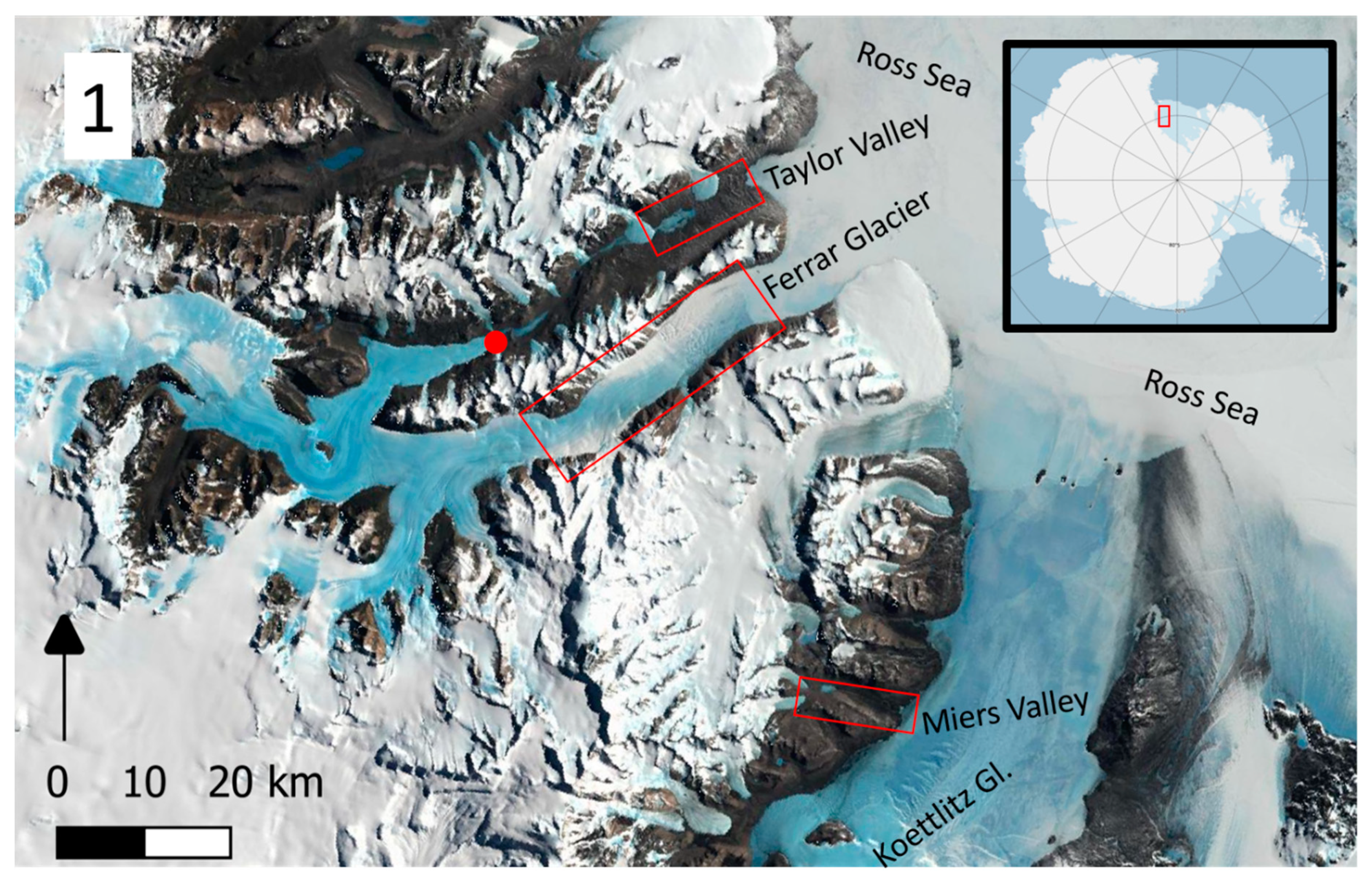
2. Setting and Methods

The MDV represent the largest ice-free region of Antarctica [34]. The region contains several major, relatively ice-free valleys that open to the ocean (Figure 1). Despite perennial cold, hyper-arid conditions [35] liquid water exists at the surface in ice-covered lakes, seasonal streams and shallow groundwater systems [36]. The largest valleys are former fjords that were inundated by the sea during the Neogene [37]. Much of the liquid in the MDV lake basins exists as brine. There is also evidence of subsurface liquid. Blood Falls is a subglacial outflow of hypersaline brine at the terminus of Taylor Glacier in Taylor Valley [38]. Multiple lines of evidence show this brine to be subglacially sourced [28,39]. Geochemistry of brine collected at Blood Falls suggests cryoconentrated seawater with modification from rock-water interaction and evaporation [25,26,38,40]. The brine from Blood Falls also hosts a metabolically active [25] and diverse microbial community that is distinct from the surrounding glacier ice [41]. Together with the extended rock-water interactions, the metabolic activity of microorganisms can facilitate mineral weathering in the subsurface, leading to high solute loads in some groundwaters. Blood Falls brine is hypersaline and rich in reduced iron (97% of iron species exist as Fe(II)) [25]. Recent geophysical surveys have provided evidence that Blood Falls is the surface expression of a deeper, regional salty aquifer [28,39,42]. Currently, Blood Falls is the only known surface discharge of Antarctic subglacial waters and therefore provides insight into the chemistry and biology of other potential subsurface brines observed in the MDV [28].
An airborne electromagnetic (AEM) survey was flown in the MDV region in November 2018 using the SkyTEM312 system, as a follow up to a proof-of-concept 2011 AEM survey [28,39,44]. The SkyTEM312 system is an airborne transient-electromagnetic (TEM) sensor and consists of a rigid frame approximately 20 by 30 m in dimension on which the various system components are mounted. The entire system is suspended and flown beneath a helicopter allowing efficient data collection over extensive regions. It employs a dual moment transmitter with an area of 342 m2. For the low-moment, the transmitter coil has 2 turns, a peak current of ~6 amps (A), and a repetition frequency of 210 hertz (Hz). For the high-moment, the transmitter coil has 12 turns, a peak current of ~110 A, and a repetition frequency of 30 Hz. The use of a dual moment transmitter balances high-resolution in the shallow subsurface with large depth penetration [45], where the subsurface can be imaged to depths up to ~600–700 m in certain conditions, such as when a conductive aquifer underlies resistive materials like frozen ground or glaciers. The AEM system flown in 2018 has significant improvements over the 2011 system including larger transmit moments and a receiver with improved sensitivity. Together these advances translate to an improved depth penetration/resolution, as well as an aerodynamic frame capable of achieving greater flying speeds of ~80–110 km/h. The collected low and high-moment data presented here included time gates from 26 μs to 1.39 ms and 392 μs to 10.7 ms, respectively.
TEM measurement involves energizing a transmit loop (i.e., ramping a current up to a peak value) and then ramping down the current in the transmit loop as rapidly as possible. When ramping the current down, a time-varying magnetic field is produced in the subsurface which induces eddy currents that propagate downwards and outwards away from the sensor. These eddy currents in turn generate a secondary magnetic field. The time variation of the secondary magnetic field is measured using a receiver coil mounted on the frame flown beneath the helicopter. The decaying secondary magnetic field produces decaying voltage signals. Further details concerning the TEM method are in Chapter 6 of Kirsch.
The result of an AEM survey is a data volume consisting of suites of measured EM field decay curves collected along densely sampled profiles. The raw data are used to constrain inverse models of subsurface electrical resistivity in the surveyed area. In this work, AEM data is inverted using a laterally constrained 30-layer inversion [46] implemented within the Aarhus Workbench software. Resistivities produced using a smooth inversion scheme are presented here. The resulting images of subsurface resistivity are presented as 2D depth slices, where the resistivity structure along a profile is visualized using a colormap (where the x- and y-axes represent distance along the profile and depth, respectively). In the presented profiles, the depth of investigation (DOI) is calculated using the approach outlined in [47]. Data below the depth of investigation are displayed as semi-transparent, and the resistivity profiles beneath these depths are not interpreted because it is considered unreliable. Where the subsurface resistivity structure at any depth cannot produce a signal that exceeds the noise level of the instrument, the data are culled and no models are inverted. In these cases the subsurface can be considered to be very resistive down to the depth of investigation. In a high polar desert most near-surface materials (e.g., glacier ice, frozen ground) have very high electrical resistivity. Hence, the AEM system excels at detecting liquid water in this environment, particularly high-salinity, low resistivity liquid brines. In cold regions, where production of authigenic clays during chemical weathering of silicates is slow, electrical resistivity is largely a function of the presence or absence of liquid water, which carries electrolytic ions. In our study region, the majority of liquid water present exists as a cryoconcentrated brine either at the surface or at depth. The process of cryoconcentration transfers water molecules from liquid phase to solid phase, while largely excluding dissolved ions from the newly formed ice crystals and concentrating them in the remaining liquid. Hence, cryoconcentration enhances the electrical contrast between solid and liquid phases of water. Cryoconcentrated brines, in turn, exist as a liquid at temperatures well below 0 °C and therefore can occur closer to the surface than would be possible for a freshwater groundwater system. In terms of electrical resistivity, subsurface brines correspond to low resistivity anomalies in the resistivity profiles. In contrast, subsurface regions containing no unfrozen water/brine, such as glaciers or permafrost, appear as areas of high resistivity.
An airborne electromagnetic platform is very well-suited to subsurface mapping in Antarctica. The surface is cold and arid, consequently a ground-based DC resistivity system would have difficulty achieving electrical contact with the surface. An inductive electromagnetic system (such as the SkyTEM312) does not require direct electrical contact with the ground. The absence of direct ground contact (both in terms of electrical contact and in respect to the fact that the system is suspended in air) is also valuable in protected areas where a ground-based survey risks disturbance of environmentally sensitive areas. An airborne platform also allows for rapid and dense data collection. An expansive AEM dataset, like the one collected by members of this team in November 2018, can provide insights into regional-scale hydrogeology of the MDV. To achieve similar coverage using ground-based methods would be infeasible given constraints on time, logistics, labor, safety considerations, and environmental accessibility.
Unlike a ground or sea-based DC survey, the AEM system cannot penetrate to great depths beneath seawater, as the highly-conductive medium strongly attenuates the signal as it propagates through the seawater. However, in Antarctica, the presence of sea ice limits the practicality of performing an off-shore DC survey. Another important distinction between DC and TEM surveys is that the greatest penetration occurs near the center of the profile for the DC survey, reducing to shallower depths near the edges of the profiles. In contrast, the TEM survey, even at a single site, can penetrate to depths up to 600–700 m depending on subsurface resistivity structure. As a result, AEM surveys can maintain large penetration depths all the way to the coastal margin. Note that the employed inversion of AEM data is based on 1D-physics for the forward model, which limits the ability to describe strongly 3D resistivity structures. One example of such a 3D-effect occurs at the coastal margins when the survey is flown perpendicularly to the coast. In locations where strong 3D-effects are identified during data processing stages, the data is culled and excluded from subsequent inversions (i.e., it does not influence the displayed profiles). Typically, this requires culling data roughly 150–250 m on either side of the coast.

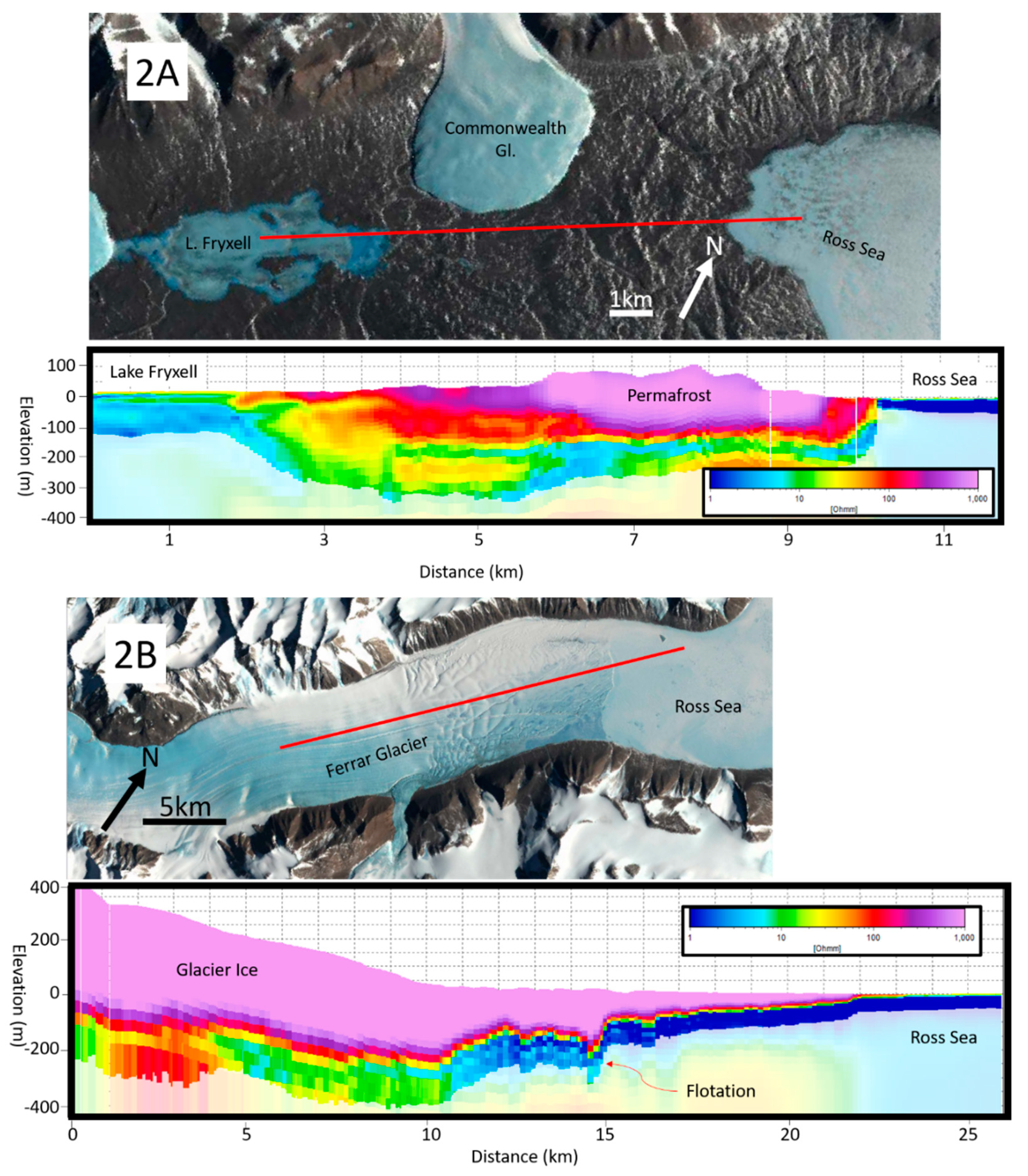
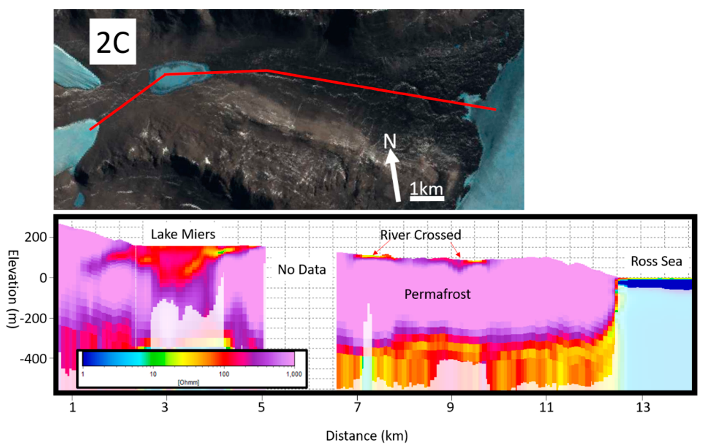
3. Results and Discussion

We collected approximately 3500 line kilometers of AEM data during 11 days of production. This survey spanned inland and coastal areas; one major focus was the connection between previously identified terrestrial brine aquifers and the ocean. We identify three representative settings where subsurface brines are in contact with ocean water and may be exchanging through SGD:
(1)
Lower Taylor Valley, where Lake Fryxell is connected to a deeper aquifer through a talik (unfrozen region) beneath the lake. This aquifer connects to the Ross Sea. This system is overlaid by permafrost between Lake Fryxell and the Ross Sea. (Figure 2A)
(2)
Ferrar Glacier, where subglacial brines have an open connection directly into the Ross Sea. (Figure 2B)
(3)
Miers Valley, where subpermafrost brines occur roughly at sea level but under a thin (and likely growing) layer of permafrost. (Figure 2C)
The extreme cold and aridity of Antarctica slow down hydrologic cycling of water and challenge our normal assumptions of the factors governing hydrogeologic processes. Here, most water exists as a slowly moving solid. Pattyn [33] estimated that the average basal melting rate beneath the Antarctic ice sheet is about 5–6 mm/year, which is an approximately two orders of magnitude less than average precipitation rates on other continents, of which only a portion may infiltrate to become groundwater. Because of this slow recharge rate, average residence times for groundwater in Antarctica can be expected to be a few orders of magnitude longer than on other continents, perhaps on the scale of millions of years in the slowest cycling portions [25]. This, in addition to the cryoconcentration process discussed previously, would allow for extended water-rock interactions and acquisition of high solute concentration, which changes fundamental water properties. Indeed, in our study region, the groundwater must be saltier, colder and denser than seawater [48,49,50,51]; therefore the primary endogenic driver of SGD (buoyant instability) is shut off. Moreover, osmotic pressures are reversed from the conditions expected in a freshwater hydrogeologic system. Oceanic processes increasing efficacy of SGD in other settings are somewhat reduced because the near-perennial sea ice mutes wave pumping and wave set up. Tidal pumping remains a factor, but largely recirculates seawater [52].
While tidal pumping and wave processes can be enormous contributors to SGD flux exchange [53], oceanic processes only recirculate and mix seawater with meteoric groundwater, mobilizing a modest amount of new solutes in every cycle. Subglacial water that is solute-rich [54], such as in the observed case for the source brine to Blood Falls [26], has undergone prolonged concentration, rock-water interaction, and microbial modification which, as described above, has saturated the brine with ions including reduced iron [25] and silica [26]. Movement of this solute rich brine into proglacial systems can impact productivity and nutrient cycling by potentially providing limited nutrients such as silica and iron. Therefore, it is important to consider Darcian flow, which transports groundwater and its attendant solutes from areas of high hydropotential to low—typically toward the ocean. Darcian flow moves hypersaline brines from land to sea without recirculation of seawater, and therefore can deliver hyperconcentrated bioavailable nutrients like dissolved (reduced) iron from their long-term reservoir to the coastal zone. Darcian Flow is described by Darcy’s Law:
Q = K   A   d h d l
where Q is the discharge (m3/s), K is the hydraulic conductivity (m/s), A is the cross-sectional area across which discharge occurs (m2), and dh/dl is the hydraulic head gradient (unitless, change in hydraulic head over distance, both in the units of length) [55].
Order of magnitude estimates of Darcian Flux can be derived for the settings observed in our study region (e.g., Figure 2A–C). Hydraulic conductivity can vary by many orders of magnitude and is particularly poorly constrained in this setting, rendering other uncertainties in gradient or area moot. Both the Ferrar Glacier and Taylor Valley represent former Miocene age fjords filled with marine diamictons and glacial drift [37]. We estimate the hydraulic conductivity using Hazen’s Relationship [56,57]:
K = C (D10)2
where C is an empirical constant (typically ~1 to report K in cm/s), and D10 is the is the diameter of the finest 10% of grains (in mm). Using the grain size records of Dry Valley Drilling Project (DVDP) boreholes [58], we estimate that a representative hydraulic conductivity of the brine carrying sediments could be of order 10−8 m/s. This estimate is in line with tabulated ranges of hydraulic conductivity in glacial tills [55,59], although it should be noted that conductivities can range over many orders of magnitude, and can be greatly enhanced by the presence of fractures. In a bulk flow setting, preferential flow through zones of higher conductivity may enhance the overall conductivity; similarly, clay or ice rich zone decrease conductivity. Drilling in the MDV has resulted in underpressurized and overpressurized wells, indicating heterogeneity in conductivities [60,61]. Without direct measurements beyond grain size and given the high sensitivity (power 2) to that grain size, we suggest that our estimate of hydraulic conductivity at 10−8 m/s should be considered only accurate to within an order of magnitude (i.e., between 10−7 and 10−9 m/s).

3.1. Surface Slope Driven Darcian Flow

Most MDV aquifers are confined by permafrost over at least some of their area. An example of this is seen in Lower Taylor Valley from Lake Fryxell to the Ross Sea (Figure 2A), where a subsurface aquifer connects Lake Fryxell to the Ross Sea by a 20 m head drop (dh) over 6500 m (dl), or or a dh/dl of 0.003. Assuming the average density of the water column from Lake Fryxell surface to aquifer basement is more dense than sea water, the dh/dl will be a little greater than this. Based on the presence of the lowest resistivities, the aquifer has a saturated thickness of 50 m and is about 2000 m wide, resulting in a, conservatively estimated 100,000 m2 cross sectional area (A). The estimated flux (Q) is therefore of the order of 100 m3/year (between 10 and 1000 m3/year when using the range for hydraulic conductivity estimated above).
Changes in lake level can significantly change the local hydraulic gradient. MDV lakes have fluctuated dramatically in the Quaternary [62]. The Fryxell basin, which is currently occupied by Lake Fryxell at close to sea level, may have been occupied by a proglacial freshwater lake (Lake Washburn) at the end of the Last Glacial Maximum that existed up to 78 masl (contained by a saddle after the Ross Ice Sheet retreated) [62,63]. This would have roughly quadrupled the hydraulic gradient toward the ocean (i.e., 380 m3/year as our best estimate or 38–3800 m3/year using the range of hydraulic conductivities). Conversely, a postulated late Holocene desiccation of Lake Fryxell [64] could have dropped the elevation of the lake below sea level, increased the salinity due to evapoconcentration, and completely reversed the gradient, driving groundwater flow inland and creating submarine groundwater recharge.
In a subglacial confined aquifer, such as under the Ferrar Glacier (Figure 2B) the horizontal head gradient, dh/dl, can be estimated as the drop in head over a distance. Without direct measurement, this is difficult to know with certainty, but an upper bound is to assume the glacier is at flotation and that the hydropotential of basal water is 90% of the ice thickness [65]. In the case of Ferrar Glacier, over the length scale over which brine is detectable, the data show a maximum drop of 300 m over 12,000 m, or 1 in 40. The saturated zone is about 4000 m wide and 50 m thick, or about 200,000 m2 in cross sectional area. Due to the higher gradient in hydraulic head, a glacier like Ferrar could produce SGD of the order of 1500 m3/year (or a range of 150–15,000 m3/year). Ferrar Glacier is moderately steep and marine terminating, making it the most representative setting for East Antarctica coastal margins out of the three example settings chosen here from our study area.
Pressurized, confined aquifers can even be found in the absence of any visible slope. Overpressurized brines have been found by boreholes throughout the MDV region on land [44,60] and underneath the McMurdo Sound [61]. Layers of frozen permafrost, as well as low permeability clay-rich layers, are capable of confining overpressurized aquifers and thus extending hydraulic head some distance from the up-gradient reservoir. This could allow transport of SGD farther out to sea with prolonged sediment-water interaction, allowing for the delivery of reduced iron to greater distance offshore before it is oxidized by ocean water and becomes insoluble.

3.2. Volume Expansion Driven Darcian Flow Due to Permafrost Growth

In Miers Valley (Figure 2C), thick permafrost overlies brine in a small valley that opens to Koettlitz Glacier and the ocean. The surface slope is small, but the expansion of downward-freezing permafrost could be driving some groundwater flux to the ocean. A ~30 m higher sea level in the MDV region during the mid-Holocene could have exposed higher valley sediments to saltwater [66], which has since been freezing down at rates currently estimated to be mm per year [67]. The volume expansion of water upon freezing can pressurize groundwater and expel it toward the ocean without any gravity-driven head. Since volume expansion of water upon freezing is about 10%, freezing at rates of 1 mm/year should ‘push’ groundwater out at rates of ca. 0.1 mm/year. For a valley that is about 10 km long and 3 km wide, this would result in a groundwater outflow of the order of 3000 m3/year. This process has the potential to link SGD output from ice-free regions of coastal Antarctica to climate changes, in that it would tend to occur transiently during periods of climate cooling and associated permafrost growth. Additionally, there is evidence that similar to Lake Fryxell basin, Miers Valley was occupied by a large paleolake at the end of the Last Glacial Maximum [62]. This would significantly alter the hydraulic gradient towards the ocean and the flux of SGD.

3.3. Darcian Flow as a Transmitter of Nutrients on a Continental Scale

Estimated fluxes of Darcian SGD are low in the MDV, due to low hydraulic conductivities, low driving gradients, and slow freezing. For example, the specific discharge of SGD at Ferrar Glacier is estimated to be about 1‰ of the ice discharge at the terminus. However, brines in the region are hyper-concentrated with ions [25,26,27], allowing for relatively high solute transport nonetheless. In contrast to West Antarctica, interior East Antarctica is predicted to have overall lower basal melting and is largely surround by zones of net freezing near the coasts where the ice is thin but surface temperatures are cold [33]. This ‘confining ring’ of cold-based ice sheet margin helps to cryoconcentrate groundwater before it reaches the coast (Figure 3). Thus, a low flux, high concentration groundwater scenario may be representative of much of coastal East Antarctica, and some parts of West Antarctica (e.g., Mary Byrd Land).
Recently, the first observationally constrained estimate of groundwater (as a combination of submarine and subglacial discharge) flux to the ocean from Antarctica was made in the West Antarctic Peninsula [68]; no estimates have been made in locations representative of other glacial and climatic regimes on the continent. Pattyn [33] modeled melting and freezing at the base of Antarctic Ice Sheet and estimated that 65 km3/year of liquid water is produced at the ice base, equivalent to 5.3 mm/year melt continent-wide. In Antarctica, this basal melt is the equivalent to liquid precipitation on other, non-ice-covered continents. On average, groundwater recharge rates on other continents represent ca. 30% of total precipitation rates [69]. In the absence of other constraints, we assume the same ratio and obtain ca. 20 cubic kilometers per year as an approximate estimate of the overall Antarctic groundwater recharge rate. The remaining 45 cubic kilometers per year of meltwater is assumed to run off relatively rapidly through systems of subglacial streams and rivers [70]. Assuming no significant change in groundwater storage, this 20 km3/year represents the approximate annual continent-wide groundwater discharge rate, too. The total volume of shallow, active groundwater in Antarctica is estimated to be of the order of 1 million km3 [70]; which at a discharge rate of 20 km3/year requires a residence time of approximately 50,000 year. The groundwaters detected in our study area are probably much older than 50,000 year, given the timescales required to achieve such high salinity through rock-water interaction and cryoconcentration. It has been hypothesized that they have remained subglacially isolated for a few million years [25]. Using our prior estimates of subsurface brine volume in the Taylor Valley (ca. 0.3–0.6 km3 assuming 20–40% of sediment porosity [28]), this kind of residence time would be compatible with SGD flux rates from this valley of ca. 100–200 m3/year, which is reasonably close with our independently calculated modern Darcian flux of groundwater. Hence, we infer that the subsurface brines imaged by our AEM survey represent the fraction of Antarctic groundwater that overturns significantly more slowly than average and has residence time closer to millions of years rather than 50,000 years. Absent any constraints, we assume for illustration purposes that these old, concentrated, sluggish groundwaters represent 5% of the 20 km3/year groundwater flux on the continent. This estimate is, of course, chosen partly of convenience to estimate that 1 km3/year of hypersaline groundwater flows to the ocean. It can serve as reference value for future researchers of this problem, who with further data may have reason to estimate saline groundwater flux as greater or less than (the order of) 1 km3/year.
Past analyses of subglacial nutrient flux [21,22] have focused on the relatively highly dynamic subglacial hydrologic system, in which basal meltwater fluxes are high at the interface of ice with underlying geology, but waters that have been sampled from such settings [71] are many orders of magnitude more dilute than the subsurface brines found in the MDV. Wadham and others [21] suggested an upper bound on iron flux by taking high concentrations from Blood Falls brine [25] and applying them to the maximum Antarctic runoff suggested by Pattyn’s [33] basal melt model. Instead, we propose that the conditions for high subglacial hydrologic flux are necessarily opposed to having a high concentration of dissolved ions, and that it is more reasonable to use our estimated slow (1 km3/year) SGD fluxes with the high concentration brines. Wetter, higher flux systems will have shorter water-rock interactions and are reasonably expected to be more dilute.
We present estimates of flux of Fe and Si through such hyperconcentrated SGD in Table 1, which is modeled after Table 2 in Reference [21]. We introduce new, direct englacial samples of the Blood Falls source brine from [26], which are believed by the authors to be more representative than the Blood Falls outflow measurements reported by [25] and used by Wadham and others [21]. For comparison, we include fluxes as calculated by the maximum basal melting scenario, although we feel this is unrealistic, as discussed above. Such a scenario was presented as an upper bound by Wadham and others [21]. We estimate that coastal East Antarctica may receive on the order of 170 Gg/year (based on Blood Falls outflow concentrations) to 20 Gg/year (based on englacial brine concentrations) of soluble iron through submarine groundwater discharge, with higher confidence in the lower value determined from more accurate englacial sampling. Interestingly, these values are very similar to Wadham’s intermediate and low flux estimates, respectively, which use similar high flux, but assumes a lower solute concentrations more representative of deep glacial groundwater [21]. Similarly, we estimate that Si flux is closer to Wadham and others’ [21] low flux estimate, for the same reasons. This hints at the reciprocity between concentration and flux of subglacial fluids. We propose that these two endmember hydrologic systems (high flux, low concentration; and low flux, high concentration) should be studied in the future with recognition of their distinct geochemical and hydrologic characteristics and origins.

4. Conclusions

AEM resistivity can rapidly detect brines in the cryosphere if they are present within 100s of meters of the surface. The MDV provide a good test case because they contain very concentrated brine largely unshielded by thick ice, making it easy to image areas of potential SGD. Before AEM surveys, observations of liquid groundwater in the MDV were limited to point observations from the DVDP borehole data [74], sporadic sampling of Blood Falls outflow [25,38] or the near-surface expression of its subglacial reservoir [26], and shallow groundwater flows in the form of water tracks [36]. Using AEM, Mikucki and others [28] showed widespread liquid brine in the MDV, but the 2011 survey had sparse spatial coverage along the coast. The 2018 AEM survey fills in gaps that not only confirms groundwater connection between terrestrial groundwater reservoirs and the ocean, but also allows us to estimate potential SGD fluxes, which is critical for understanding nutrient fluxes to the ocean. We estimate that approximately 1 km3/year (~2% of total continent-wide basal melt) of hypersaline groundwater exits Antarctica as SGD and is chemically similar to that detected in the MDV. We predict that this slow, salty flux carries approximately 20 Gg/year of Fe and 14 Gg/year of Si to the Southern Ocean through SGD, particularly in East Antarctica, where the MDV are examples of the widespread net freezing at the coastal margin. This subglacial setting stands in marked contrast to the dilute, high flux conditions expected in most of West Antarctica, but is has the potential to be similarly as significant for nutrient transport.

Author Contributions

Conceptualization, S.T.; Data curation, E.A.; Formal analysis, D.G. and N.F.; Funding acquisition, S.T., P.D., J.M., R.V. and E.A.; Investigation, H.D.; Project administration, S.T., P.D., J.M. and E.A.; Writing—original draft, N.F. and D.G.; Writing—review & editing, P.D., J.M., K.F.M. and H.D., R.V.

Funding

This research was funded by National Science Foundation Grant numbers 1643687 and 1644187.

Acknowledgments

We are grateful to PAE Antarctic support personnel for providing helicopter services that enabled our data collection. Logistical support for this project in Antarctica was provided by the U.S. National Science Foundation through the U.S. Antarctic Program. Efficient collection of large quantities of TEM data was possible thanks to experience and professionalism of our field operations manager, Lars Jensen. We are also grateful for the helpful commentary of two anonymous reviewers, and guidance from the editors of Hydrology. Thanks, also, to William Altman for guidance.

Conflicts of Interest

The authors declare no conflict of interest.

References

  1. Burnett, W.C.; Bokuniewicz, H.; Huettel, M.; Moore, W.S.; Taniguchi, M. Groundwater and Pore Water Inputs to the Coastal Zone. Biogeochemistry 2003, 66, 3–33. [Google Scholar] [CrossRef]
  2. Moore, W.S. The Effect of Submarine Groundwater Discharge on the Ocean. Ann. Rev. Mar. Sci. 2009, 2, 59–88. [Google Scholar] [CrossRef] [PubMed]
  3. Simmons, G.M. Importance of submarine groundwater discharge (SGWD) and seawater cycling to material flux across sediment/water interfaces in marine environments. Mar. Ecol. Prog. Ser. 1992, 84, 173–184. [Google Scholar] [CrossRef]
  4. Santos, I.R.; Eyre, B.D.; Huettel, M. The driving forces of porewater and groundwater flow in permeable coastal sediments: A review. Estuar. Coast. Shelf Sci. 2012, 98, 1–15. [Google Scholar] [CrossRef]
  5. Kwon, E.Y.; Kim, G.; Primeau, F.; Moore, W.S.; Cho, H.-M.; DeVries, T.; Sarmiento, J.L.; Charette, M.A.; Cho, Y.-K. Global estimate of submarine groundwater discharge based on an observationally constrained radium isotope model. Geophys. Res. Lett. 2014, 41, 8438–8444. [Google Scholar] [CrossRef]
  6. Lecher, A. Groundwater Discharge in the Arctic: A Review of Studies and Implications for Biogeochemistry. Hydrology 2017, 4, 41. [Google Scholar] [CrossRef]
  7. Lecher, A.L.; Chien, C.-T.; Paytan, A. Submarine groundwater discharge as a source of nutrients to the North Pacific and Arctic coastal ocean. Mar. Chem. 2016, 186, 167–177. [Google Scholar] [CrossRef] [Green Version]
  8. Frederick, J.M.; Buffett, B.A. Effects of submarine groundwater discharge on the present-day extent of relict submarine permafrost and gas hydrate stability on the Beaufort Sea continental shelf. J. Geophys. Res. Earth Surf. 2015, 120, 417–432. [Google Scholar] [CrossRef]
  9. DeFoor, W.; Person, M.; Larsen, H.C.; Lizarralde, D.; Cohen, D.; Dugan, B. Ice sheet-derived submarine groundwater discharge on Greenland’s continental shelf. Water Resour. Res. 2011, 47. [Google Scholar] [CrossRef]
  10. Uemura, T.; Taniguchi, M.; Shibuya, K. Submarine groundwater discharge in Lützow-Holm Bay, Antarctica. Geophys. Res. Lett. 2011, 38. [Google Scholar] [CrossRef]
  11. Lecher, A.L.; Kessler, J.; Sparrow, K.; Garcia-Tigreros Kodovska, F.; Dimova, N.; Murray, J.; Tulaczyk, S.; Paytan, A. Methane transport through submarine groundwater discharge to the North Pacific and Arctic Ocean at two Alaskan sites. Limnol. Oceanogr. 2016, 61, S344–S355. [Google Scholar] [CrossRef]
  12. Mahowald, N.M.; Baker, A.R.; Bergametti, G.; Brooks, N.; Duce, R.A.; Jickells, T.D.; Kubilay, N.; Prospero, J.M.; Tegen, I. Atmospheric global dust cycle and iron inputs to the ocean. Glob. Biogeochem. Cycles 2005, 19. [Google Scholar] [CrossRef]
  13. Slomp, C.P.; Van Cappellen, P. Nutrient inputs to the coastal ocean through submarine groundwater discharge: controls and potential impact. J. Hydrol. 2004, 295, 64–86. [Google Scholar] [CrossRef] [Green Version]
  14. Tréguer, P.; Jacques, G. Dynamics of nutrient and phytoplankton and cycles of carbon, nitrogen and silicon in the Southern Ocean: a review. Polar Biol. 1992, 12, 149–162. [Google Scholar] [CrossRef]
  15. Moore, J.K.; Abbott, M.R. Phytoplankton Chlorophyll Distributions and Primary Production in the Southern Ocean. J. Geophys. Res. 2000, 105, 28709–28722. [Google Scholar] [CrossRef]
  16. De Baar, H.J.W.; Buma, A.G.J.; Nolting, R.F.; Cadée, G.C.; Jacques, G.; Tréguer, P.J. On iron limitation of the Southern Ocean: experimental observations in the Weddell and Scotia Seas. Mar. Ecol. Prog. Ser. 1990, 65, 105–122. [Google Scholar] [CrossRef]
  17. Martin, J.H.; Gordon, R.M.; Steve, E.F.; Fitzwater, S.E. Iron in Antarctic waters. Nature 1990, 345, 156–158. [Google Scholar] [CrossRef]
  18. Gerringa, L.J.A.A.; Alderkamp, A.-C.; Laan, P.; Thuróczy, C.-E.; De Baar, H.J.W.W.; Mills, M.M.; van Dijken, G.L.; van Haren, H.; Arrigo, K.R. Iron from melting glaciers fuels the phytoplankton blooms in Amundsen Sea (Southern Ocean): Iron biogeochemistry. Deep Sea Res. Part II Top. Stud. Oceanogr. 2012, 71–76, 16–31. [Google Scholar] [CrossRef]
  19. Thuróczy, C.-E.; Alderkamp, A.-C.; Laan, P.; Gerringa, L.J.A.; Mills, M.M.; Van Dijken, G.L.; De Baar, H.J.W.; Arrigo, K.R. Key role of organic complexation of iron in sustaining phytoplankton blooms in the Pine Island and Amundsen Polynyas (Southern Ocean). Deep Sea Res. Part II Top. Stud. Oceanogr. 2012, 71–76, 49–60. [Google Scholar] [CrossRef]
  20. Raiswell, R.; Benning, L.G.; Tranter, M.; Tulaczyk, S. Bioavailable iron in the Southern Ocean: The significance of the iceberg conveyor belt. Geochem. Trans. 2008, 9, 7. [Google Scholar] [CrossRef]
  21. Wadham, J.L.; De’ath, R.; Monteiro, F.M.; Tranter, M.; Ridgwell, A.; Raiswell, R.; Tulaczyk, S. The potential role of the Antarctic Ice Sheet in global biogeochemical cycles. Earth Environ. Sci. Trans. R. Soc. Edinburgh 2013, 104, 55–67. [Google Scholar] [CrossRef]
  22. Wadham, J.L.; Tranter, M.; Skidmore, M.; Hodson, A.J.; Priscu, J.; Lyons, W.B.; Sharp, M.; Wynn, P.; Jackson, M. Biogeochemical weathering under ice: Size matters. Global Biogeochem. Cycles 2010, 24, 3025. [Google Scholar] [CrossRef]
  23. McKay, C.P.; Hand, K.P.; Doran, P.T.; Andersen, D.T.; Priscu, J.C. Clathrate formation and the fate of noble and biologically useful gases in Lake Vostok, Antarctica. Geophys. Res. Lett. 2003, 30. [Google Scholar] [CrossRef]
  24. Michaud, A.B.; Dore, J.E.; Achberger, A.M.; Christner, B.C.; Mitchell, A.C.; Skidmore, M.L.; Vick-Majors, T.J.; Priscu, J.C. Microbial oxidation as a methane sink beneath the West Antarctic Ice Sheet. Nat. Geosci. 2017, 10, 582–586. [Google Scholar] [CrossRef]
  25. Mikucki, J.A.; Pearson, A.; Johnston, D.T.; Turchyn, A.V.; Farquhar, J.; Schrag, D.P.; Anbar, A.D.; Priscu, J.C.; Lee, P.A. A Contemporary Microbially Maintained Subglacial Ferrous “Ocean”. Science 2009, 324, 397–400. [Google Scholar] [CrossRef]
  26. Lyons, W.B.; Mikucki, J.A.; German, L.A.; Welch, K.A.; Welch, S.A.; Gardner, C.B.; Tulaczyk, S.M.; Pettit, E.C.; Kowalski, J.; Dachwald, B. The Geochemistry of Englacial Brine from Taylor Glacier, Antarctica. J. Geophys. Res. Biogeosci. 2019, 124, 633–648. [Google Scholar] [CrossRef]
  27. Mikucki, J.A.J.; Foreman, C.C.M.; Sattler, B.; Berry Lyons, W.; Priscu, J.C. Geomicrobiology of Blood Falls: An Iron-Rich Saline Discharge at the Terminus of the Taylor Glacier, Antarctica. Aquat. Geochem. 2004, 10, 199–220. [Google Scholar] [CrossRef]
  28. Mikucki, J.A.; Auken, E.; Tulaczyk, S.; Virginia, R.A.; Schamper, C.; Sørensen, K.I.; Doran, P.T.; Dugan, H.; Foley, N. Deep groundwater and potential subsurface habitats beneath an Antarctic dry valley. Nat. Commun. 2015, 6, 6831. [Google Scholar] [CrossRef] [Green Version]
  29. Tréguer, P.J. The Southern Ocean silica cycle. Comptes Rendus - Geosci. 2014, 346, 279–286. [Google Scholar] [CrossRef]
  30. Green, W.J.; Stage, B.R.; Preston, A.; Wagers, S.; Shacat, J.; Newell, S. Geochemical processes in the Onyx River, Wright Valley, Antarctica: Major ions, nutrients, trace metals. Geochim. Cosmochim. Acta 2005, 69, 839–850. [Google Scholar] [CrossRef]
  31. Tulaczyk, S.; Mikucki, J.A.; Siegfried, M.R.; Priscu, J.C.; Barcheck, C.G.; Beem, L.H.; Behar, A.; Burnett, J.; Christner, B.C.; Fisher, A.T.; et al. WISSARD at Subglacial Lake Whillans, West Antarctica: scientific operations and initial observations. Ann. Glaciol. 2014, 55, 51–58. [Google Scholar] [CrossRef] [Green Version]
  32. Joughin, I.R.; Tulaczyk, S.; Engelhardt, H.F. Basal melt beneath Whillans Ice Stream and Ice Streams A and C, West Antarctica. Ann. Glaciol. 2003, 36, 257–262. [Google Scholar] [CrossRef] [Green Version]
  33. Pattyn, F. Antarctic subglacial conditions inferred from a hybrid ice sheet/ice stream model. Earth Planet. Sci. Lett. 2010, 295, 451–461. [Google Scholar] [CrossRef]
  34. Levy, J. How big are the McMurdo Dry Valleys? Estimating ice-free area using Landsat image data. Antarct. Sci. 2013, 25, 119–120. [Google Scholar] [CrossRef]
  35. Doran, P.T.; McKay, C.P.; Clow, G.D.; Dana, G.L.; Fountain, A.G.; Nylen, T.; Lyons, W.B. Valley floor climate observations from the McMurdo dry valleys, Antarctica, 1986-2000. J. Geophys. Res. Atmos. 2002, 107. [Google Scholar] [CrossRef]
  36. Levy, J.S.; Fountain, A.G.; Gooseff, M.N.; Welch, K.A.; Lyons, W.B. Water tracks and permafrost in Taylor Valley, Antarctica: Extensive and shallow groundwater connectivity in a cold desert ecosystem. Geol. Soc. Am. Bull. 2011, 123, 2295–2311. [Google Scholar] [CrossRef]
  37. Sugden, D.; Denton, G.; Marchant, D. Landscape evolution of the Dry Valleys, Transantarctic Mountains: Tectonic implications. J. Geophys. Res. 1995, 100, 9949–9967. [Google Scholar] [CrossRef]
  38. Keys, J. Saline discharge at the terminus of the Taylor Glacier. Antarct. J. US 1979, 14, 82–85. [Google Scholar]
  39. Foley, N.; Tulaczyk, S.; Auken, E.; Schamper, C.; Dugan, H.; Mikucki, J.; Virginia, R.; Doran, P. Helicopter-borne transient electromagnetics in high-latitude environments: An application in the McMurdo Dry Valleys, Antarctica. Geophysics 2015, 81, WA87–WA99. [Google Scholar] [CrossRef]
  40. Lyons, B.W.; Frape, S.K.; Welch, K.A. History of McMurdo Dry Valley lakes, Antarctica, from stable chlorine isotope data. Geology 1999, 27, 527. [Google Scholar] [CrossRef]
  41. Campen, R.; Kowalski, J.; Lyons, W.B.; Tulaczyk, S.; Dachwald, B.; Pettit, E.; Welch, K.A.; Mikucki, J.A. Microbial diversity of an Antarctic subglacial community and high-resolution replicate sampling inform hydrological connectivity in a polar desert. Environ. Microbiol. 2019. [Google Scholar] [CrossRef]
  42. Badgeley, J.A.; Pettit, E.C.; Carr, C.G.; Tulaczyk, S.; Mikucki, J.A.; Lyons, W.B. An englacial hydrologic system of brine within a cold glacier: Blood Falls, McMurdo Dry Valleys, Antarctica. J. Glaciol. 2017, 63, 387–400. [Google Scholar] [CrossRef] [Green Version]
  43. Bindschadler, R.; Vornberger, P.; Fleming, A.; Fox, A.; Mullins, J.; Binnie, D.; Paulsen, S.J.; Granneman, B.; Gorodetzky, D. The Landsat Image Mosaic of Antarctica. Remote Sens. Environ. 2008, 112, 4214–4226. [Google Scholar] [CrossRef]
  44. Dugan, H.A.; Doran, P.T.; Tulaczyk, S.; Mikucki, J.A.; Arcone, S.A.; Auken, E.; Schamper, C.; Virginia, R.A. Subsurface imaging reveals a confined aquifer beneath an ice-sealed Antarctic lake. Geophys. Res. Lett. 2015, 42, 96–103. [Google Scholar] [CrossRef]
  45. Sørensen, K.I.; Auken, E. SkyTEM—A new high-resolution transient electromagnetic system. Explor. Geophys. 2004, 35, 191–199. [Google Scholar] [CrossRef]
  46. Auken, E.; Christiansen, A.V. Layered and laterally constrained 2D inversion of resistivity data. Geophysics 2004, 69, 752. [Google Scholar] [CrossRef]
  47. Christiansen, A.V.; Auken, E. A global measure for depth of investigation. Geophysics 2012, 77, WB171. [Google Scholar] [CrossRef]
  48. McGinnis, L.D.; Stuckless, J.S.; Osby, D.R.; Kyle, P.R. Gamma Ray, Salinity, and Electric Logs of DVDP Boreholes. Dry Val. Drill. Proj. 1981, 33, 95–108. [Google Scholar]
  49. McGinnis, L.D.; Nakao, K.; Clark, C.C. Geophysical Identification of Frozen and Unfrozen Ground Antarctica. In Permafrost: North American contribution [to the] Second International Conference; National Academy of Sciences: Washington, DC, USA, 1973; pp. 136–146. [Google Scholar]
  50. McGinnis, L.D.; Osby, D.R.; Kohout, R. Paleohydrology inferred from salinity measurements on Dry Valley Drilling Project cores from Taylor Valley, Antarctica. Antarct. Geosci. 1982, 4, 1133–1138. [Google Scholar]
  51. McGinnis, L.D.; Jensen, T.E. Permafrost-Hydrogeologic Regimen in Two Ice-Free Valleys, Antarctica, from Electrical Depth Sounding. Quat. Res. 1971, 409, 389–409. [Google Scholar] [CrossRef]
  52. Prieto, C.; Destouni, G. Quantifying hydrological and tidal influences on groundwater discharges into coastal waters. Water Resour. Res. 2005, 41. [Google Scholar] [CrossRef] [Green Version]
  53. Li, L.; Barry, D.A.; Stagnitti, F.; Parlange, J.-Y. Submarine groundwater discharge and associated chemical input to a coastal sea. Water Resour. Res. 1999, 35, 3253–3259. [Google Scholar] [CrossRef] [Green Version]
  54. Skidmore, M.; Tranter, M.; Tulaczyk, S.; Lanoil, B. Hydrochemistry of ice stream beds-Evaporitic or microbial effects? Hydrol. Process. 2010, 24, 517–523. [Google Scholar]
  55. Freeze, R.A.; Cherry, J.A. Groundwater; Prentice-Hall: New York, NY, USA, 1979; ISBN 0-13-365312-9. [Google Scholar]
  56. Hazen, A. Some physical properties of sands and gravels. Mass. State Board of Health. 24th Annu. Rep. 1892, 539–556. [Google Scholar]
  57. Salarashayeri, A.F.; Siosemarde, M. Prediction of soil hydraulic conductivity from particle-size distribution. World Acad. Sci. Eng. Technol. 2012, 61, 454–458. [Google Scholar]
  58. Powell, R. Sedimentation Conditions in Taylor Valley, Antarctica, Inferred from Textural Analysis of DVDP Cores. In Dry Valley Drilling Project; American Geophysical Union: San Francisco, CA, USA, 2013; Volume 33, pp. 331–349. ISBN 9781118664643. [Google Scholar]
  59. Domenico, P.A.; Schwartz, F.W. Physical and Chemical Hydrogeology; John Wiley and Sons: New York, NY, USA, 1990. [Google Scholar]
  60. McGinnis, L.D. Artesian well at Don Juan Pond. Antarct. J. US 1979, 14, 26–27. [Google Scholar]
  61. Falconer, T.; Pyne, A.; Wilson, D.; Levy, R.; Nielsen, S.; Petrushak, S. Operations overview for the ANDRILL Southern McMurdo Sound Project, Antarctica. Terra Antart. 2008, 15, 41–48. [Google Scholar]
  62. Hendy, C.H. Late Quaternary Lakes in the McMurdo Sound Region of Antarctica. Geogr. Ann. Ser. A Phys. Geogr. 2004, 82, 411–432. [Google Scholar] [CrossRef]
  63. Hall, B.B.L.; Denton, G.G.H.; Hendy, C.H. Evidence from Taylor Valley for a grounded ice sheet in the Ross Sea, Antarctica. Geogr. Ann. Ser. A Phys. Geogr. 2000, 82, 275–303. [Google Scholar] [CrossRef]
  64. Lyons, W.B.B.; Tyler, S.W.W.; Wharton, R.A.A.; McKnight, D.M.M.; Vaughn, B.H.H. A Late Holocene desiccation of Lake Hoare and Lake Fryxell, McMurdo Dry Valleys, Antarctica. Antarct. Sci. 1998, 10, 247–256. [Google Scholar] [CrossRef]
  65. Cuffey, K.M.; Paterson, W.S.B. The Physics of Glaciers; Academic Press: New York, NY, USA, 2010; ISBN 008091912X. [Google Scholar]
  66. Hall, B.L.; Baroni, C.; Denton, G.H. Holocene relative sea-level history of the Southern Victoria Land Coast, Antarctica. Glob. Planet. Change 2004, 42, 241–263. [Google Scholar] [CrossRef]
  67. Osterkamp, T.E.; Burn, C.R. Permafrost. Encycl. Atmos. Sci. 2003, 1717–1729. [Google Scholar]
  68. Null, K.A.; Reide Corbett, D.; Crenshaw, J.; Peterson, R.N.; Peterson, L.E.; Lyons, W.B. Groundwater discharge to the western Antarctic coastal ocean. Polar Res. 2019, 38. [Google Scholar] [CrossRef]
  69. Döll, P.; Fiedler, K. Global-scale modeling of groundwater recharge. Hydrol. Earth Syst. Sci. 2008, 12, 863–885. [Google Scholar] [CrossRef] [Green Version]
  70. Priscu, J.C.; Tulaczyk, S.; Studinger, M.; Kennicutt II, M.C.; Christner, B.C.; Foreman, C.M. Antarctic subglacial water: Origin, evolution, and ecology. In Polar Lakes and Rivers; Oxford University Press: Oxford, England, 2008; ISBN 9780199213887. [Google Scholar]
  71. Christner, B.C.; Priscu, J.C.; Achberger, A.M.; Barbante, C.; Carter, S.P.; Christianson, K.; Michaud, A.B.; Mikucki, J.A.; Mitchell, A.C.; Skidmore, M.L.; et al. A microbial ecosystem beneath the West Antarctic ice sheet. Nature 2014, 512, 310–313. [Google Scholar] [CrossRef] [PubMed]
  72. Gosselin, D.C.; Harvey, F.E.; Frost, C.D. Geochemical evolution of ground water in the Great Plains (Dakota) Aquifer of Nebraska: Implications for the management of a regional aquifer system. Groundwater 2001, 39, 98–108. [Google Scholar] [CrossRef]
  73. Kim, M.-J.; Nriagu, J.; Haack, S. Arsenic species and chemistry in groundwater of southeast Michigan. Environ. Pollut. 2002, 120, 379–390. [Google Scholar] [CrossRef]
  74. Cartwright, K.; Harris, H. Hydrogeology of the Dry Valley Region, Antarctica. Antarct. Res. Ser. 1981, 33. [Google Scholar] [CrossRef]
Figure 1. The McMurdo Dry Valleys Region Landsat Image of Antarctica (LIMA) high-resolution virtual mosaic [43]. The red dot denotes the location of Blood Falls at the terminus of Taylor Glacier. Inset shows the study region (red box) on a map of Antarctica.
Hydrology 06 00054 g001
Figure 2. (A) AEM cross section of Lower Taylor Valley showing the connection between Lake Fryxell and the Ross Sea by a talik and conductive aquifer. Low resistivity regions are interpreted as liquid brines; (B) AEM cross section of Ferrar Glacier showing subglacial brine connecting to the Ross Sea; and (C) AEM cross section of Miers Valley. Brine can be detected underneath thick permafrost, and this brine appears to be in contact with the Ross Sea.
Hydrology 06 00054 g002aHydrology 06 00054 g002b
Figure 3. Basal melting conditions in Antarctica, adapted and simplified from Reference [33]. Freezing conditions at the base are indicated by blue and high (above average) melting rates (<6 mm/year) are indicated by yellow. West Antarctica has relatively overall basal melt rates, while East Antarctica has lower melts rates. The margin of the East Antarctic ice sheet contains extensive zones of net freezing, and this ‘confining ring’ is proposed by us to be a zone of cryoconcentration near the coast. The red star marks the study area.
Hydrology 06 00054 g003
Table 1. Estimated fluxes of Fe and Si through continent-wide SGD, after Table 2 from [21]. Sources: Reported concentrations and calculated values from fields marked (a) are from Reference [21]; concentrations from fields marked (b) are from Reference [26] and the unmarked calculated values are scaled after Table 2 from Reference [21]. [21] cites and slightly rounds its Fe concentrations from Reference [25] and its Si concentrations from References [72,73].
IonConcentration (µM)Flux of Ions (Gg/year)
At 1 km3/year SGDAt 65 km3/year SGD
Fe(II) (Blood Falls outflow, filtered to remove insoluble particulates) a300017011,000 a
Fe (total iron, direct englacial sample, unfiltered) b476301700
Fe(II) (direct englacial sample, filtered to remove insoluble particulates) b351201300
Si a600171100 a
Si b48414900

