Abstract
Perennial snowfields in Gates of the Arctic National Park and Preserve (GAAR) in the central Brooks Range of Alaska are a critical component of the cryosphere. They serve as habitat for an array of wildlife, including caribou, a species that is crucial as a food and cultural resource for rural subsistence hunters and Native Alaskans. Snowfields also influence hydrology, vegetation, permafrost, and have the potential to preserve valuable archaeological artifacts. By deriving time series maps using cloud computing and supervised classification of Landsat satellite imagery, we calculated areas and evaluated extent changes. We also derived changes in elevations of the perennial snowfields that remained stable for at least four years. For the study period of 1985 to 2017, we found that total areas of perennial snowfields in GAAR are decreasing, with most of the notable changes in the latter half of the study period. Equilibrium areas, or bright areas, of the snowfields are shrinking, while ablation, or dark areas, are growing. We also found that the snowfields occur at higher elevations over time. Climate change may be altering the distribution, elevation, and extent of perennial snowfields in GAAR, which could affect caribou populations and subsistence lifestyles in rural Alaska.
1. Introduction
Pronounced warming of the climate is driving significant physical and ecological changes throughout the Arctic cryosphere [1,2,3,4], including both a shortening of the annual duration of seasonal snow cover [5], as well as retreat and loss of glaciers and perennial snowfields. Perennial snowfields, like glaciers, are masses of snow and ice that persist for many years and form through accumulation and compaction of seasonal layers of snow. However, in contrast to glaciers, these features never grow thick enough to flow under the influence of gravity. They are most persistent where the climatological snowline intercepts subtle terrain and plateau topography in the Arctic [6], and where preferential snow deposition occurs and topography limits exposure to solar radiation [7]. Preferential snow deposition involves the uneven distribution of snow cover due to orographic influences on winter precipitation, wind-influenced snow transport, and avalanches [8,9,10,11,12]. Perennial snowfields are vulnerable to climate changes because they are strongly controlled by the height of the summer freezing level in the atmosphere.
Perennial snowfields are an important component of the Arctic cryosphere because they influence hydrology, downslope vegetation [13], bedrock weathering through freeze-thaw cycles [14], soil temperatures, and permafrost distribution [15]. They are also important ecosystems for an array of birds and mammal species [16]. Reductions in the extent of both glaciers and snowfields during the late twentieth century [17] have been observed across the Arctic, including in Gates of the Arctic National Park and Preserve (GAAR) in the central Brooks Range of Alaska [18]. Changes in perennial snowfields could influence caribou in GAAR, since caribou often flock to these snowfields in the summer to stay cool and to avoid mosquitos [19,20,21,22]. Caribou are crucial to traditional subsistence for indigenous Native Alaskan people [23,24,25,26,27]. The loss of perennial snowfields in GAAR may also have the potential to reveal well-preserved archeological artifacts and ancient animal remains with significant cultural and paleoecological value, as have been found in other alpine snow and ice fields in Alaska and Canada [28,29,30,31,32,33]. Federal agencies in Alaska also consider perennial snowfields to be important cultural, hydrological, and ecological resources [34,35].
Perennial and seasonal snow and ice encompass a substantial portion of the planet, and by utilizing satellite imagery, snow hydrologists and glaciologists can gain a better understanding of their behavior [36,37,38,39,40]. Satellite imagery and earth remote sensing are important for monitoring changes in the cryosphere, including past [6,41,42,43], present [44,45,46,47], and future behavior of seasonal and perennial snow and ice. One of the most widely used of these datasets for observing snow and ice is the National Aeronautics and Space Administration’s (NASA’s) Land Remote-Sensing Satellite System (Landsat). Landsat has been used for years to obtain information about the cryosphere [42,48,49,50,51,52,53,54,55,56,57,58], including glacier and ice sheet mapping [37,38,59,60,61,62] and the tracking of seasonal snow cover [49,63,64]. Few remote sensing studies have targeted perennial snowfields specifically, and instead, typically focus on mapping glaciers [57,58,65]. Other studies have specifically focused on the contributions of perennial snowfields to the cryosphere [6,39,41,66,67].
Automated and semi-automated multispectral glacier and land ice mapping methods are common, including supervised classification [61,68,69,70] and the Normalized Difference Snow Index (NDSI) [53,55,57,71,72]. NDSI is an effective method for mapping both seasonal [43,73] and perennial [57,58] snow and ice. NDSI is a numerical indicator that highlights snow cover over land and uses the difference of the green and short wave infrared spectral bands divided by the sum of the same band. Snow and clouds reflect most of the incident radiation in the visible band, but snow absorbs most incident short wave radiation and clouds do not, distinguishing snow from clouds.
Glaciers, perennial snowfields, and seasonal snow are all important hydrological components of the quickly shifting cryospheric landscape. Perennial snowfields, in particular, are the main component of the cryosphere in GAAR. Remote sensing of these frozen features is important for monitoring their present conditions, as well as for modeling both past and future changes. Therefore, the purpose of this research is to quantify changes in perennial snowfield extents, by studying Landsat satellite imagery of GAAR in the central Brooks Range in Alaska. To quantify snowfield changes, four objectives were addressed in this study: (1) identify and map perennial snowfield minimum extents by applying NDSI to Landsat imagery across GAAR during the available period of record (1985–2017); (2) apply supervised classification to those snowfields to derive time series maps of two sub-classes of perennial snowfields, including equilibrium areas (brightly colored areas that indicate snowfields are maintaining or increasing area) and ablation areas (darker regions that indicate snowfields are shrinking); (3) quantify perennial snowfield areas, including calculations of total, equilibrium, and ablation areas, and testing for statistical significance (trends) in area changes; and (4) quantify changes in point elevations (PEs) of the perennial snowfields. We determined PEs by placing a 2 × 2 km grid across the study area of GAAR and derived the lowest elevation point in each grid cell for snowfields that were persistent for at least four years during pre-determined quartile time periods, using a digital elevation model (DEM). The 2-km2 grid was used because it was the finest resolution that could be overlain onto a land area as vast as GAAR and still be a reasonably efficient computational task for our computing methods.
2. Study Area
This study focuses on perennial snowfields in Gates of the Arctic National Park and Preserve (GAAR), which is a United States (US) federally managed land unit in northern Alaska (Figure 1). GAAR is the northernmost, and second largest, national park in the US, with its entirety lying north of the Arctic Circle and covering an area of about 34,287 km2. It is located in the central portion of the Brooks Range Mountains and was chosen as the focus area of this study, rather than the entire Brooks Range, because, as a national park, it is managed differently than other areas of this mountain range. In addition, the Brooks Range covers a vast area where the climate varies from region to region [74]. These differences can affect the behavior and persistence of perennial snowfields.
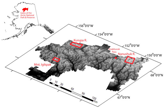
Figure 1.
Study area map of Gates of the Arctic National Park and Preserve (GAAR) in the central Brooks Range in Alaska. Top left shows location of GAAR relative to state of Alaska, USA. Bottom shows a detailed close-up of GAAR, including the 5m Digital Elevation Model (DEM) used in the study. Also seen are the three localized areas that were evaluated in more detail; including Nanushuk River, Mount Igikpak, and Kurupa River.
Additionally, three detailed local study areas were used to represent changes in perennial snowfield extents at scales finer than can effectively be seen across such a large study area as GAAR. The local areas were chosen based on the most concentrated clusters of perennial snowfields and included the Nanushuk River, Mount Igikpak, and Kurupa River study areas (Figure 1). The mean elevations of the Nanushuk River, Mount Igikpak, and Kurupa River study areas are, respectively, 1511, 1271, and 1473 m. Their mean slope angles are 28°, 29°, and 26°, respectively, and their mean aspects are SE, SW, and S, respectively.
GAAR was created in 1980 as part of the Alaska National Interest Lands Conservation Act (ANILCA), which has had a major impact on subsistence caribou hunting for rural Native Alaskan communities. The ability of very remote communities to secure food sources through local hunting has serious consequences for their socio-economic and cultural sustainability. This includes caribou hunters in the remote Native Alaskan village of Anaktuvuk Pass, which is located inside of GAAR, as well as caribou hunters across the North Slope of Alaska. Land management decisions influence local rural peoples’ ability to hunt, and climate change affects perennial snow and ice, which in turn, may affect wildlife populations, such as the caribou that these communities depend on for subsistence. In this way, both changes in perennial snowfields and in land management decisions have an impact on local people living in this area.
A portion of the eastern boundary of the park is located about 8 km from the Dalton Highway (Alaska State Highway 11), with the westernmost part of the Arctic National Wildlife Refuge (ANWR) located about 16 km further east. The Middle Fork of the Koyukuk River is located between GAAR and the Dalton Highway, with the Trans-Alaska Pipeline running parallel to the Dalton. Anaktuvuk Pass is located on a Native land withholding inside GAAR (Elevation: 683 m; Coordinates: 68.1433°N, 151.7358°W). Access to the park by non-residents is limited by the terrain and lack of roads. Extreme inter-seasonal temperature range and low annual precipitation characterize the climate of GAAR. Up until the 1990s, temperatures could drop as low as −38 °C in the winter, but they could also reach as high as 22 °C [74] for a short time in summer, due in part to nearly continuous daylight during the mid-summer. Over the 33-year period of this study, however, the weather stations in and around GAAR recorded minimum temperatures as low as −30 °C and maximum temperatures as high as 16 °C, with annual mean temperatures around −14 and −5.5 °C, respectively (ncdc.noaa.gov).
GAAR has very few large glaciers remaining [18], especially in comparison to other regions of Alaska, but has many rivers that are fed by a combination of ground water sources and seasonal and perennial snow and ice melt. The majority of perennial ice and snow cover in GAAR consists of either the many small perennial snowfields that are sparsely distributed across mid-to-high elevation valleys and north-facing aspects of the Brooks Range, or of perennial aufeis. Aufeis is ice that accumulates during the winter over rivers and lakes, formed by upwelling of water behind ice dams, or by ground water discharge. The perennial portion of aufeis persists in low lying valleys year round where there is less exposure to solar radiation.
3. Data Sources and Methods
3.1. Data and Imagery Used
NASA Landsat imagery was accessed and analyzed using Google Earth Engine (GEE), a cloud-computing-based platform for planetary scale geospatial analysis [75]. GEE integrates a super computer, satellite and reanalysis data, and a Javascript coding environment. GEE contains the full Landsat archive, with pixel-scale co-registration of all scenes. The data used are from the Landsat Tier 1 (T1) top of atmosphere (TOA) reflectance collections for missions 4, 5, 7, and 8, which include a period of study from 1985 through 2017 (Figure 2). GEE’s T1 TOA product is pre-calculated and includes calibration of TOA reflectance. Calibration coefficients are extracted from the image metadata [76].
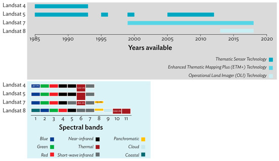
Figure 2.
Landsat missions years of availability in Gates of the Arctic National Park and Preserve (GAAR); satellite payload sensor technologies; spectral bands; pixel spatial scales of each band analyzed in this study.
Acquisition and dissemination of Landsat data is currently a joint effort between NASA and the United States Geological Survey (USGS), with the first Landsat satellite being launched in 1972. Replacement satellites have been launched throughout the decades, with each containing new technology, allowing for additional spectral bands [77]. The evolution of Landsat sensors includes the Thematic Mapper (TM), the Enhanced Thematic Mapper (ETM+), the Operational Land Imager (OLI), and the Thermal Infrared Sensor (TIRS) technologies [77]. Some years of Landsat 4 and 5 data were not of useable quality because there were missing tiles within the study area of GAAR, including all years before 1985. Multiple spatial scales, spectral bands, and temporal scales of the imagery were analyzed in this study (Figure 2).
Also used in this study was a 5-m resolution digital elevation model (DEM). It was important to obtain an accurate DEM for calculation of point elevations (PEs) and for other topographic corrections associated with shadowing from mountainous terrain. Our DEM is primarily based on ArcticDEM, released in 2016 from the University of Minnesota’s Polar Geospatial Center (pgc.umn.edu/data/arcticdem). In 2017, Candela et al. [78] performed an accuracy study on this DEM, wherein it was registered to seasonally subsetted ICESat elevations (Ice, Cloud, and Land Elevation Satellite). The vertical accuracy of ArcticDEM was obtained from the statistics of the fit to ICESat and averaged −0.01 ± 0.07 m. ArcticDEM has very good spatial coverage for GAAR, but is missing some data. Our DEM is a combination of ArcticDEM and the University of Alaska Fairbanks’ Geographic Information Network of Alaska’s (GINA’s) IfSAR (interferometric synthetic aperture radar) dataset, which was also obtained in 2016, via aircraft mounted radar detection. The IfSAR data were used to fill in missing data from ArcticDEM. IfSAR has a vertical accuracy of 3 m and a horizontal accuracy of 12.2 m (ifsar.gina.alaska.edu).
3.2. Data Preprocessing
The methods described below are also depicted schematically in the flow chart in Figure 3. Two primary datasets, containing annual cloud-free mosaics, were generated from: (1) Landsat 4 and 5 (L4/L5), and (2) Landsat 7 and 8 (L7/L8). Landsat tiles located entirely or partially within GAAR during a 6-week summer season of interest (1 July to 15 August) were included. This summer season is defined here as the time of snowfield minimum extent (late summer) when perennial layers are revealed beneath the seasonal snow cover. The Landsat 4 and 5 (L4/L5) dataset was temporally discontinuous, as some years of data were missing for the study area, including 1993, 1994, 1996, 1997, 1998, and 2000–2004. The data were first cloud-masked using a simple and standardized approach to arrive at a cloud score per pixel [79]. In order to verify that clouds were not actually snow, the cloud score also included a calculation of the NDSI for each pixel [43]. The cloud-masking algorithm then created a derived image of cloud scores corresponding to each pixel, to screen out excessively cloudy pixels. We also used the quality band (QA) available for L7/L8 to exclude pixels designated as “cirrus” or “cloud”.
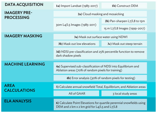
Figure 3.
Schematic Flow chart of methodology used in the study. 1a) Pre-processed Landsat data from missions 4, 5, 7, and 8, for summer (1 July to 15 August) in GAAR were acquired from GEE. 1b) 5 m DEM was constructed from ArcticDEM and IfSAR data. 2a) Landsat imagery was cloud masked and mosaicked to obtain one imager per summer. 2b) Mosaicked Landsat 7 and 8 datasets were pan-sharpened to 15 m scale with pan-chromatic band and HSV technique. 3a) Non-snow land cover types were masked out, including surface water using NDWI, 3b) elevations below 900 m to eliminate aufeis, and 3c) very steep terrain that cannot hold snow with slope angles over 55 degrees. 3d) Remaining image evaluated using NDSI and 25% darkest pixels (shadows) removed using a percentile function. 4a) NDSI areas sub-classified into ablation and equilibrium areas using supervised classification and 4b) error analysis. 5) Snowfield areas calculated annually for total, equilibrium, and ablation areas, across GAAR and in three local study areas. 6) Lowest Point Elevations (PEs) calculated using DEM and 2 km2 grid for each snowfield area remaining stable for at least four years.
There are striping gaps in Landsat 7 [80,81,82]. We corrected them using a striping mask by detecting pixels with reflectance values at or near zero, and mosaicking those pixels with others georeferenced from the same tile, but imaged during a different pass of the satellite. Our annual mosaic for each dataset was created by calculating the median TOA reflectance value from all non-cloud-covered pixels available per summer for each pixel. This technique also mitigated the darkening effects of mountain shadows and cloud shadows. We pan-sharpened the L7/L8 data with the pan-chromatic 15-m scale band using the Hue-Saturation-Value (HSV) approach [83,84].
The final preprocessing step was to mask out areas of the images that would never contain snow in the summer. The two land cover types removed included (1) areas of liquid water and (2) areas with elevations and slope angles unlikely to retain snow during the summer. Liquid water was determined using the Normalized Difference Water Index (NDWI) with a threshold value of 0.3, as well by using the Global Surface Water Recurrence dataset [85].
GEE has a 32-day NDWI composite made from Tier 1 orthorectified scenes, using the computed TOA reflectance [86]; however, we used our own calculations of NDWI per annual summer mosaic for the masking process, as our study time period was different than the 32-day composite. For the areas unlikely to retain summer snow, we included low elevation valleys below the perennial snow line, as well as extremely steep terrain with slope angles over 55 degrees, which were determined using the 5-m DEM created for GAAR. Aufeis has a similar spectral signature as perennial snowfields, and so, it was also necessary to mask out aufeis as part of the pre-processing. This was achieved when the low elevation valleys were removed, since aufeis typically occurs as part of rivers located in the valleys.
3.3. Imagery Analysis
To find the snow that remained stable throughout the entire study period, areas designated as snow by NDSI were used to calculate a forward gradient (NDSIn–NDSIn+1) and a reverse gradient (NDSIn+1–NDSIn) for each dataset (L4/L5 and L7/L8). These values were used to compute the minimum gradient between successive images. We calculated NDSI for our specific mosaics used in this study, rather than using an existing Landsat snow cover product, since our 15-m pan-sharpened L7/L8 data would have been difficult to compare with existing snow cover data at the 30-m scale, such as the Tier 3 Fractional Snow Cover (FSC) product [87].
A percentile function was applied where the darkest 25% of each pixel in the snowfield was removed from the bottom 75th percentile (darkest 75% of each pixel). This helped mitigate the effects of mountain shadows and cloud shadows. Also, since GAAR is so far north, the sun remains high for most of the day in the summer. The sun’s incident angle is quite small, and shadows have less influence on the brightness of images here. Areas of perennial snow were derived for quartiles within the period of record for each of the two datasets, with L4/L5 quartiles consisting of L45_Q1 from 1985 to 1988, L45_Q2 from 1989 to 1992, L45_Q3 from 2005 to 2007, and L45_Q4 from 2008 to 2011. The L7/L8 quartiles included L78_Q1 from 1999 to 2003, L78_Q2 from 2004 to 2008, L78_Q3 from 2009 to 2013, and L78_Q4 from 2014 to 2017. Due to the temporally discontinuous nature of the L4/L5 data, 1995 and 1999 were excluded from the quartiles. This was the basis for defining “perennial” in our study. There are few other studies that have attempted to define the minimum age of a snowfield that could be considered perennial. For those studies that have broached this topic, the minimum number of years needed to define a snowfield as perennial range from two [8,88] to 20 [89]. For our study, we considered snowfields as perennial if they persisted year-round for at least four years.
To determine equilibrium and ablation areas of the perennial snowfields, we used supervised classification on those areas designated as snow by NDSI, which involved the use of training and testing pixels [67,90]. This sub-classification routine involved two classes: equilibrium areas with high NDSI values, and ablation areas with low NDSI values. This was done as an additional metric to the overall net changes in the perennial snowfield extents in order to investigate the effects of seasonal variability, and to quantify snowfield areas that may have remained stable, but have transitioned from viable snow (equilibrium) to vulnerable or thinner snow (ablation). Thirty percent of the pixels per class were used for testing and error assessment, while 70% were used for training. Equilibrium and ablation area training and testing pixels were randomly derived, using high NDSI values (0.8 to 1.0) and low NDSI (0.4 to 0.5), respectively. These values were designated using an iterative process, rather than by simply applying a threshold value, to allow for the machine learning process to expedite the classification of areas with NDSI values between 0.5 and 0.8 and to pinpoint areas misclassified as snow.
Extent changes across GAAR were then calculated for total, equilibrium, and ablation areas annually. The nonparametric Mann-Kendall statistic for testing of a trend was calculated for the annual changes in the three localized study areas, for both L4/L5 and L7/L8, and Theil–Sen trend lines were applied. We assessed the accuracy of the classification procedure by quantifying the errors of commission (EC) and the errors of omission (EO) associated with classifying the land cover types as Not Snow, Equilibrium Areas, or Ablation Areas. Accuracy percentage and the kappa index (K) were found in GEE using error algorithms. K, a common statistic in remote sensing, measures agreement for qualitative (categorical) items and takes into account the possibility of the agreement occurring by chance [91,92,93,94]. Error matrices were created and testing pixels were used to generate a confusion matrix for each year, including overall accuracy percentage, K, EC, and EO (Table 1a,b). Finally, we quantified changes in point elevations (PEs) using a 2-km2 grid for snowfields that were persistent for at least four years (quartiles). PEs of quartile perennial snowfields for equilibrium and ablation areas in L4/L5 and L7/L8 were derived. Coordinates of the lowest elevations in each cell for each class were obtained from the DEM.

Table 1.
Supervised sub-classification error assessment results.
4. Results
The overall accuracy assessment of the equilibrium and ablation area sub-classification (Table 1a,b) indicates relatively high accuracy. Accuracy percentages range from 100% to 70%, although the majority of 19 years analyzed in the procedure fall within the 100–90% range. Six out of the 19 years, or about 30%, had overall accuracies below 90%. The results of the kappa index (K) analysis were more variable than overall accuracy, with a majority of K values ranging from 1.00 to 0.60. Six out of the 19 years, or about 30%, had K values below 0.60, with all of those years being in the L7/L8 dataset. Extent changes across GAAR were calculated for total, equilibrium, and ablation areas annually. A summary of these results, comparing the first year of the study period (1985: L4/L5 30-m data) to the last year (2017: L7/L8 15-m data), including coverage change percentages within each cell of a 1-km2 grid for 1985 and 2017 is provided in Figure 4.
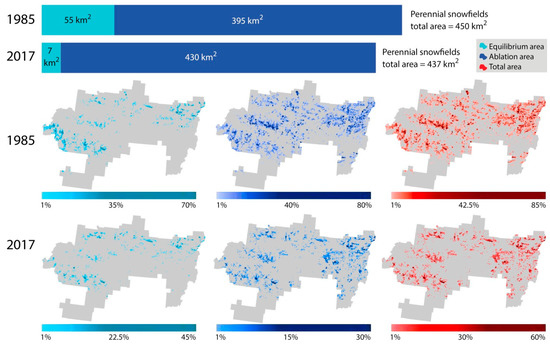
Figure 4.
Annual summer season (1 July–15 Aug) perennial snowfield areal extent changes from the beginning of the study time period (1985, derived from the 30 m scale Landsat 4 and 5 imagery) to the end of the study time period (2017, derived from the 15 m scale Landsat 7 and 8 imagery). The top panel shows net changes in the total area between 1985 and 2017, including changes in the sub-classified equilibrium (bright) areas and ablation (dark) areas of the snowfields. The bottom panel shows changes in percent cover between 1985 and 2017 per 1 km2 grid cell across the entire area of GAAR for equilibrium, ablation, and total areas.
Annual snowfield extent changes across all of GAAR show an overall decrease in snowfield area of 13 km2 between 1985 and 2017, although larger seasonal variations existed within that time period (Figure 4). While net total area between 1985 and 2017 decreased only slightly, the composition of the perennial snowfields shifted notably towards more ablation areas and less equilibrium areas. There was a larger 48 km2 decrease in viable equilibrium areas, indicating that the composition of the snowfields shifted largely towards more ablation areas, which increased by 35 km2. Percentage changes in all of the coverage maps indicate substantial decreases within the 1-km2 grid for equilibrium, ablation, and total areas across GAAR (Figure 4). Snowfield area extent changes in GAAR can be seen in the annual summer season (1 July–15 August) perennial snowfield minimum extent areas and in the Mann-Kendall Theil–Sen trend lines, within the three detailed study areas for Nanushuk River, Mount Igikpak, and Kurupa River (Figure 5: 30-m L4/L5; Figure 6: 15-m L7/L8).
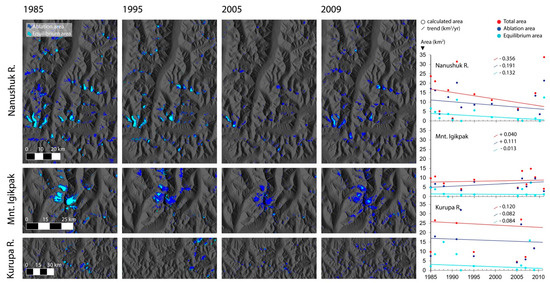
Figure 5.
Annual summer season (1 July–15 Aug) perennial snowfield minimum extent time series maps derived from the 30 m scale Landsat 4 and 5 imagery (L4/L5), showing several example years in the three localized study areas of Nanushuk River, Mount Igikpak, and Kurupa River. The maps depict changes in overall snowfield coverage, as well as changes in equilibrium areas (light blue) and in ablation areas (dark blue). The accompanying graphs show the extent changes in the three study areas quantitatively, including calculated areas for each summer from observed extent changes, as well as trends in the area changes. The trend lines are derived from the nonparametric Mann-Kendall Theil Sen’s statistical approach, for total extent changes, as well as for equilibrium and ablation area changes.
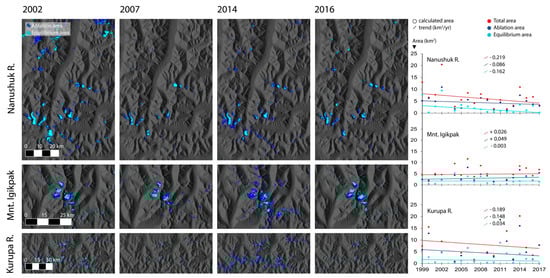
Figure 6.
Annual summer season (1 July–15 Aug) perennial snowfield minimum extent time series maps derived from the 15 m scale Landsat 7 and 8 imagery (L7/L8), showing several example years in the three localized study areas of Nanushuk River, Mount Igikpak, and Kurupa River. The maps depict changes in overall snowfield coverage, as well as changes in equilibrium areas (light blue) and in ablation areas (dark blue). The accompanying graphs show the extent changes in the three study areas quantitatively, including calculated areas for each summer from observed extent changes, as well as trends in the area changes. The trend lines are derived from the nonparametric Mann-Kendall Theil Sen’s statistical approach, for total extent changes, as well as for equilibrium and ablation area changes.
Both area-trend line graphs, as well as mapped extent changes, are provided as sets of time series for all three study areas (Figure 5). Example years shown for L4/L5 include 1985, 1995, 2005, and 2009, with equilibrium areas mapped in light blue and ablation areas in dark blue, overlain onto the DEM. Most of the trend lines indicate that snowfield extents decreased over the L4/L5 time period, except in Mount Igikpak, where the equilibrium areas remained relatively constant, while ablation areas slightly increased, resulting in a slight increase in overall snowfield extent. In the Nanushuk River area, trends indicate that snow-covered areas here slightly decreased over the summer seasons within the discontinuous time period of 1985–2011. Calculated areas in Nanushuk River for the L4/L5 data indicate that both equilibrium and ablation areas decreased slightly, resulting in an overall total area decrease. This is in contrast to the Mount Igikpak study area where snow-covered areas slightly increased over the summer seasons within L4/L5. Calculated areas in Mount Igikpak indicate that both equilibrium and ablation areas increased slightly, resulting in an overall total area increase. Like the Nanushuk River area, the Kurupa River snow-covered areas remained stable or slightly decreased over this time period. Areas for L4/L5 in Kurupa River indicate that equilibrium areas remained stable, while ablation areas slightly decreased, resulting in an overall decrease.
L7/L8 is presented in a manner similar to L4/L5 (Figure 6). Example years shown for L7/L8 include 2002, 2007, 2014, and 2016. Most of the trend lines indicate that snowfield extents decreased over the L7/L8 time period, except in Mount Igikpak, where trends (and snowfield areas) remained nearly constant. In the Nanushuk River, trends indicate that snow-covered areas decreased over the summers of 1999–2017 (Figure 6). Calculated areas in Nanushuk River for L7/L8 indicate that both equilibrium and ablation areas decreased, with a more noticeable decrease in equilibrium and a very slight decrease in ablation. This resulted in an overall total area decrease for L7/L8 in the Nanushuk River area. In Mount Igikpak, trends indicate that snow-covered areas essentially remained stable. The trend in Kurupa River shows that snow-covered areas remained close to stable or very slightly decreased, including a very slight decrease in ablation areas, while equilibrium areas remained stable. It is important to note that annual minimum snowfield extent changes across GAAR, as well as in the three local study areas, may include variability from both seasonal snow pack and perennial snowfields (Figure 4, Figure 5 and Figure 6).
Lastly, scatterplots of point elevations (PEs) of perennial snowfields persistent over the four year quartile periods, including equilibrium and ablation areas, are provided (Figure 7). These include the first four-year quartile period of L4/L5 (1985–1988) and the last four years of L7/L8 (2014–2017). When PEs are grouped by latitude, Cluster A includes the Kurupa and Nanushuk rivers, and Cluster B includes Mount Igikpak. When they are grouped by longitude, Cluster C includes Kurupa River and Mount Igikpak, and Cluster D represents Nanushuk River. Elevation changes versus latitude and longitude over time show that the lowest elevations in all clusters of points in the scatterplots consistently shifted upwards between the 1985–1988 and 2014–2017 quartiles.
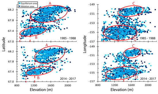
Figure 7.
Observed changes in PEs of perennial snowfields’ equilibrium and ablation areas for snowfields persistent over first four years (top panel) and last four years (bottom panel) of the study period. PEs were determined by placing a 2 km2 grid across GAAR and finding lowest elevation points in each cell for equilibrium and ablation areas. The top panel shows snowfields persisting from at least 1985 to 1988 (30 m L4/L5) and the bottom panel shows those persisting from at least 2014 to 2017 (15 m L7/L8). PE changes in latitude are on the left and changes in longitude are on the right. The encircled clusters of PEs indicate the most concentrated areas of snowfields, which correspond to the three localized areas. Cluster A is Kurupa and Nanushuk Rivers; B represents Mount Igikpak; C is Kurupa River and Mount Igikpak; D is Nanushuk River.
5. Discussion
This study quantified changes in perennial snowfield extents in GAAR in the central Brooks Range of Alaska using the Google Earth Engine (GEE) cloud-computing-based platform. Mapping snow- and ice-covered areas with GEE [95,96,97,98,99] has a much greater speed, efficiency, and accuracy than other older remote sensing software packages because GEE consists of a multi-petabyte analysis-ready data catalog co-located with a high-performance, intrinsically parallel computation service. It enables users to compute petabytes of data through an internet-accessible application programming interface (API) without having to navigate the complexities of cloud-based parallelization [75]. The assessment of our supervised classification routine performed in GEE indicates good accuracy, with the procedure being slightly more accurate in L4/L5 than in L7/L8 (Table 1a,b). By using GEE, these robust methods for detecting changes in the perennial snowfields in GAAR are open-source, with publicly available code and transparent methodologies that are repeatable. Since we performed the bulk of these analyses in GEE, the code and methods are easily shared and re-usable, as the environment in GAAR continues to change (our L4/L5 GEE code: https://code.earthengine.google.com/db00680d06e75d0a763aee62a9d6a759; our L7/L8 GEE code: https://code.earthengine.google.com/e05be7ba8f99505af418021fa715cdc2). The cloud-computing format also means this code can be run by those with limited computing resources.
5.1. Mapped and Quantified Perennial Snowfield Areas
Perennial snowfields are highly susceptible to climate change [89] and are sensitive indicators of such change. This is because snowfields are much smaller than glaciers, yet they persist longer than seasonal snow [66]. They can be quickly altered by shifts in temperature and precipitation patterns at both local and regional scales [10]. Perennial snowfields in GAAR may be particularly vulnerable to these shifts, due to the accelerated rate of climate change in the Arctic [3,4,100,101]. Snowfields are strongly influenced by many factors, including topography, wind, and exposure to solar radiation. These factors can change snowfield shape, extent, and distribution [8].
Perennial snowfields are ephemeral and susceptible to changes in weather [66] and climate [102]. It is important to consider changes in perennial snowfield extents in the context of climate, weather, and topography interactions [12]. These considerations could aid in an overall understanding of perennial snowfield behavior in response to climate change, including any feedback cycles between climate and an array of other factors such as size, exposure to sunlight, slope angle, and color or brightness. When we mapped the perennial snowfields across the extent of GAAR for both the L4/L5 and L7/L8 datasets, we saw the influence of several of these topographic factors, including the effects of cirque backwall sheltering and limited exposure to sunlight in narrow deep valleys. These features, typical of alpine terrain, provided shading from summer ablation. As our time series progressed, however, warming temperatures or lack of snow appeared to become controlling factors in the slow decrease in overall extents of perennial snowfields in GAAR.
Biologists and subsistence hunters are eager to understand why changes in populations of caribou herds occur. These changes are most likely the result of multiple environmental and biological factors, including the locations of concentrated areas of perennial snowfields in regions that caribou herds frequent [21,22,23,24,25,26]. The initial NDSI processing (Objective (1)) yielded similar geographical results in both the L4/L5 and L7/L8 imagery for the two time periods (1985–2011 and 1999–2017) (Figure 4, Figure 5, Figure 6 and Figure 7). The two datasets show the perennial snowfields to be similar in terms of spatial coverage and locations of the most concentrated clusters. The majority of the snowfields are located in extremely mountainous areas in the Northeast (NE), Southwest (SW), and Northwest (NW) corners of GAAR. This is why these locations were chosen for more detailed inspection as the localized areas of Nanushuk River (NE), Mount Igikpak (SW), and Kurupa River (NW) (Figure 1).
The Nanushuk River valley runs down the middle of the study area and Northwest-facing snowfields to both the East and West of the valley appear to lose equilibrium areas. This is especially true for the more rounded snowfields to the East. A similar glacier and perennial snowfield mapping project in 1998 in Glacier National Park also used visual comparison of co-registered satellite images to assess variations in firn lines, annual boundaries between ice and snow facies, and changes in the shape of glaciers and snowfields [66]. Like that study, the results of this research, including information regarding extent and shape changes of the snowfields, can be determined by investigating the individual clusters of perennial snowfields that are seen in more detail in the three local study areas. The time series maps summarize annual behavior and changes in extents for equilibrium and ablation areas (Figure 5 and Figure 6). In Nanushuk River, there may be some seasonal variations mixed in with perennial areas; ablation areas vary greatly and equilibrium areas decrease.
For the Mount Igikpak study area (Figure 5), the time series also indicates some seasonal variations of snow cover remaining throughout the summer, mixed in with the perennial areas. The seasonality of the ablation areas is very apparent in Mount Igikpak, indicating that some of the areas classified as perennially ablating coverage could be short-term persistent seasonal snow cover. There is a dramatic decrease in equilibrium areas in Mount Igikpak for the L4/L5 data (Figure 5), moving across the example years from 1985 to 2009. The Kurupa River area encompasses a much larger area than what is seen in Nanushuk River and Mount Igikpak. Overall, total snowfield extents decreased in Kurupa River, as was the case in Nanushuk. This can be seen in the time series for Kurupa River for the L4/L5 data, with practically zero coverage of equilibrium areas by the end of 2009.
The results of this study also have implications for archeologists working in these areas to find artifacts [28,29,30], as they may not find well-preserved specimens if in fact the snowfields are only persistent for several years at a time. The equilibrium areas were almost completely gone by the latter part of this time series, leaving mostly darker-colored ablation areas (Figure 5). This may mean that there were longer-term perennial areas in the 1980s, but that they completely disappeared by the 2000s, leaving snowfields that persisted somewhat randomly for only a summer or two. In the Nanushuk River study area (Figure 6), the time series indicates a substantial amount of equilibrium areas, which steadily decreased throughout the years, along with decreases in the ablation area extents. The Nanushuk River snowfields in 2016 show some small amounts of coverage of equilibrium areas, but the graphical results indicate almost zero coverage by 2017.
In a 1998 study in Glacier National Park by Allen, potential effects of cirque backwall sheltering of perennial snow and ice were found to provide shading from summer ablation [66] and therefore create an ideal topography. Despite this, warming temperatures (or lack of snow) appear to have eventually won out over the influences of the cirque basin in the Mount Igikpak study area. For Mount Igikpak (Figure 6), areal extents of the snowfields appear to remain annually steady across the L7/L8 time period, which can also be seen in the area calculations. There appears to have been a substantial decrease in 2010 (not shown), followed by a rebound in the latter years of this time series. This may also be an indication of high levels of seasonality in Mount Igikpak for L7/L8. In the earlier images of the L4/L5 Mount Igikpak time series, there is a substantial ablation area in a Northeastern cirque basin; however, by the end of the L4/L5, and throughout the L7/L8, this ablating snowfield all but disappears.
Some of our results also indicate that perhaps the Northwest corner of GAAR is changing more rapidly than other areas of the park. There may be a more influential and warmer climate here, as a result of documented changes in climate on Alaska’s North Slope and from changes in Arctic Ocean cycles [103,104]. In the Kurupa River area in the Northwest (our largest study area) there is substantially less areal coverage of total snowfield extent for the L7/L8 data than what was seen in the L4/L5 data (Figure 6). A quantitative correlation is not feasible between the datasets in Kurupa River, since results of the classification process are from two disparate spatial scales. However, it appears that snowfield extents substantially decreased from 1985 to 2017 in this study area, taking into account both datasets at their differing resolutions.
There are an array of stakeholders and scientists, including hydrologists, geologists, biologists, and archaeologists, who need to understand the behavior of perennial snowfields and how they are changing because of climate warming [1]. Wildlife biologists are investigating how perennial snowfields provide important habit to all sorts of different species [16]. Perennial snowfields provide a source of water for downslope vegetation, including lichen in the Brooks Range [13], which is primary forage for caribou [24,25,26]. Upon comparison of overall snowfield extent changes during the study period in GAAR, there was only a small total decrease in snowfield area between 1985 and 2017. However, there was a much larger decrease in the viable equilibrium areas, indicating that the composition of the snowfields shifted notably towards more ablation areas, which increased substantially (Figure 4). The overall percentage change in coverage also showed substantial decreases for equilibrium, ablation, and total areas (Figure 4). Both hydrologists and ecologists use quantifiable results from cryospheric research such as this in order to plan for ecological shifts, for changes in water supplies for northern communities, and for climate change adaptation [105,106].
Calculating gross snowfield extent changes for the entire park may be a useful approach for multiple natural science disciplines. However, utilizing our local detailed study areas to inspect extent changes and test for significance in those area changes could be the ideal method for other types of scientists and stakeholders. For example, archeologists and paleo-ecologists around the world are looking for cultural artifacts and paleo-ecological specimens that have remained well preserved in snow and ice for centuries or millennia [32]. Once snow and ice melt, it is critical for these scientists to retrieve such items before exposure to the elements starts to degrade artifacts [31,33]. Knowing where perennial snowfield perimeters have most recently changed at a relatively finer scale, through quantitative analyses, could help them target areas of priority for their cultural resource surveys. These types of quantifiable changes in snowfields, measured annually, could give archaeologists important information about the places they look for artifacts.
5.2. Trends in Perennial Snowfield Area Changes
It is important to note that when supervised classification was applied to annual extent changes in the snowfields, there was a probability that some of these areas were actually part of the seasonal snowpack and not necessarily perennial. Even within the designated summer season of 1 July–15 August in the Brooks Range, seasonal snowfall is possible, as well as non-typical late melt or early season re-accumulation of snow cover [74]. Keeping in mind this mixing of seasonal and perennial snow coverage signals in the annual data, Sen trend lines were calculated and applied to the results, which summarize summer snow coverage in the localized study areas. Objective (3) was to quantify perennial snowfield areas, as measured from the time series maps, and to test for statistical significance in area changes using a Mann-Kendall Theil–Sen nonparametric technique. In the Nanushuk River area, there is an overall decrease in total snowfield extents, with both equilibrium and ablation areas decreasing (Figure 5). In the Mount Igikpak study area, there was an overall slight increase in total snowfield extent for L4/L5. The equilibrium areas remained nearly constant; therefore, the increase in this study area is attributed completely to the increase in ablation areas. For the Kurupa River study area (Figure 5), overall total snowfield extents decreased, as was the case in Nanushuk River. Kurupa River, a much larger study area than the other two, had equilibrium areas that nearly disappeared by 2011.
The L7/L8 analysis for the Nanushuk River study area indicated an overall slight decrease in total snowfield extent from 1999 to 2017 (Figure 6). Equilibrium areas decreased to nearly zero by 2017, with a very slight decrease (or nearly constant coverage) in ablation areas. In Mount Igikpak (Figure 6), areas of perennial snowfields remained steady across the L7/L8 time period. There appears to have been a substantial decrease in 2010, followed by a rebound in the latter years of the time series. This may also be an indication of high levels of seasonality in Mount Igikpak, and perhaps 2010 represents the actual perennial coverage. For L7/L8, there is substantially less coverage by snowfields in Kurupa River (Figure 6) than was seen in the L4/L5 data. This could mean that the snowfield extents were gaining each winter season, but only in short-term coverage, around the perimeters of the snowfields. While the perennial snowfields were growing, the total growth could be attributed to ephemeral areas that were also ablating.
Inspecting snowfield changes is also important for permafrost research. Perennial snowfields provide insulation for permafrost-dominated landscapes [15] in many regions of the Arctic cryosphere. As permafrost thaws and permanently frozen land becomes unfrozen for the first time in human history [107,108], a quantitative understanding of how snowfield retreat in high latitude and high elevation regions is contributing to the loss of permafrost could be critical to monitoring such changes. Trends in perennial snowfield coverage could have implications for permafrost in GAAR. For both L4/L5 and L7/L8 in the Nanushuk area, snowfield coverage continued to slowly decrease over the entire 1985–2017 time period. This could signal an eventual thaw for permafrost in this part of GAAR, as the snowfields slowly lose their ability to insulate permafrost from the summer heat [109,110]. The permafrost in the Mount Igikpak area might have been less vulnerable during the study period, as snowfield coverage remained relatively stable in both L4/L5 and L7/L8, providing consistent insulation [111,112]. Permafrost may have changed most recently in the Kurupa River area, as the perennial snowfield coverage increased in L4/L5, but then decreased in L7/L8.
The more recent and finer-scale data show larger decreases in extents with very little re-growth of the snowfields for both the annual and quartile results. It is possible that these more substantial decreases in snowfield extents are an outcome of a warming Arctic [4], as the L7/L8 data represents latter years in the study area of GAAR. However, it is also important to mention that the disparate scales may be contributing to the differences in trends between the older 30-m and newer 15-m data. This is a very important potential error, and in some cases might impact the sign of the trend. The 15-m data may be a more accurate representation of the behavior of the snowfields, as these bodies of snow and ice are quite ephemeral and vulnerable to small changes due to their smaller sizes [89]. If scaling issues are the controlling factor in the results [113,114,115], the 15-m data would likely do a better job of representing changes.
5.3. Perennial Snowfield PE Changes
Deriving changes in elevations for both perennial snowfields and glaciers has been shown to be one of several effective ways for monitoring responses to climate change [116]. There are a variety of ways to measure these elevation changes for snowfields and glaciers, including the equilibrium line altitude (ELA) approach, as well as by tracking changes in the elevation of specific points. An increase in measured elevation over time generally indicates a reduction in area of the snowfield or glacier [40,59,60,66,117]. This is another important indicator of the impacts of a changing climate on the cryosphere. Elevation changes could affect the nature of the relationship that caribou and other wildlife have to these frozen features as habitable ecosystems [21,22]. This may include the ability of wildlife to physically access the terrain where snowfields remain steady throughout the summer seasons [25]. Therefore, the final objective of this study, Objective (4), is to quantify changes in point elevations (PEs) of the perennial snowfields.
The ELA approach is a classic method for tracking elevation changes of glaciers and snowfields [39,41,89]. This technique involves measuring the elevation at which mass balance is equal—where accumulation of snow is exactly balanced by ablation over a period of a year [118]. The ELA technique can be used on individual glaciers and snowfields, or it can be applied to many bodies of snow and ice to calculate changes across a broad landscape. Because GAAR is so large and contains many small perennial snowfields with geometries that change rapidly from year to year, using the ELA technique within the GEE environment proved cumbersome. Therefore, we used another method for measuring changes in elevation that could be applied uniformly across the study area. Our method involved deriving point elevations (PEs) within a grid for equilibrium and ablation areas of the snowfields.
We determined PEs by placing a 2-km2 grid across the study area of GAAR and deriving the lowest elevation point in each grid cell for snowfields that were persistent for at least four years during pre-determined quartile time periods, using the 5-m digital elevation model (DEM). Two-km2 grid cells were used in our study because this was the finest resolution that could be overlain onto a study area as large as GAAR and still be a time efficient computational task for the cloud-computing abilities of GEE. Few other studies have employed the exact method that we used, possibly because cloud computing is a newer approach to studying perennial snow and ice. However, several other glacier studies have used the approach of measuring elevation changes with discrete points both in the field [119,120], as well as with satellite and aerial photography [121,122,123].
Example scatterplots of PEs of perennial snowfields persistent over the four year quartile periods, including equilibrium and ablation areas, are provided in Figure 7. These include the first four-year period of L4/L5 (1985–1988) and the last four years of L7/L8 (2014–2017). Elevation changes versus latitude/longitude over time are shown. The various encircled clusters of PEs indicate the most concentrated areas of perennial snowfields, which correspond to the three localized study areas. While this method of clustering is somewhat up to interpretation, it appears that the lowest elevations in all clusters consistently shifted upwards between the 1985–1988 and 2014–2017 quartiles. Clusters A, B, C, and D shifted upwards about 100, 125, 150, and 50 m, respectively. Trends of upward movements in elevation indicate that the perennial snowfields are shrinking, as the highest elevations of masses of snow and ice last the longest. This could be the result of an observed increase in annual air temperatures in the Arctic, with higher rates of increase seen at higher Arctic latitudes [3,4,100,101].
6. Conclusions
The purpose of this research was to quantify changes in perennial snowfield extents in GAAR through four objectives: (1) identifying and mapping perennial snowfield minimum extents using NDSI and Landsat imagery; (2) using supervised classification to find two sub-classes of perennial snowfields, including equilibrium and ablation areas; (3) calculating perennial snowfield areas and testing for statistical significance in the changing trends; and (4) finding changes in PEs of the snowfields. The accuracy assessment of the equilibrium and ablation area sub-classification procedure indicated good accuracy, with slightly more accuracy in L4/L5 than in L7/L8.
By deriving time series maps using NDSI (Objective (1)) and supervised classification (Objective (2)), we were able to calculate changes in the total, equilibrium, and ablation areas of the snowfields. For the study period of 1985–2017, we found that the perennial snowfields in GAAR Verify tense change, though most of the notable changes in extent were in the latter half of the study period. Changes in viable equilibrium areas, or bright areas, of the perennial snowfields are shrinking much faster than total areas, and dark ablation areas are growing. Ablation areas are the most likely to melt out first, as they absorb more solar radiation. Some of these changes are the result of seasonal, inter-annual, and annual variability.
We used a Mann-Kendall Theil–Sen nonparametric statistical approach to determine the trends in extent changes of the perennial snowfields in GAAR (Objective (3)). In the Nanushuk River local study area, there was an overall decrease in total snowfield extents, with ablation areas decreasing slightly, and equilibrium areas decreasing to nearly zero by 2017. In the Mount Igikpak area, there was an overall slight increase in total snowfield extent for the L4/L5 time period, while areas remained steady during the L7/L8 period, which may be an indication of high seasonality in Mount Igikpak. In the Kurupa River area—a much larger study area than the other two—total snowfield extents decreased, with equilibrium areas nearly disappearing by 2011. For the L7/L8 time period in Kurupa River, there was substantially less coverage by snowfields than the earlier L4/L5 period.
By evaluating changes in the point elevations (PEs) of the perennial snowfields that remained stable for at least four years (Objective (4)), we were able to characterize changes in elevations of the perennial snowfields. By inspecting changes in elevation versus longitude, as well as changes in elevation versus latitude, we found that the snowfields occur at higher and higher elevations over time. Increases in PE are an additional indicator that shows that the GAAR perennial snowfields are slowly decreasing in areal extent. Further research is needed to investigate changes in perennial snowfield extent in the central Brooks Range, including the classification and evaluation of different types of satellite imagery. Since changes in snowfields are of significance to multiple stakeholders, including scientists and subsistence hunters, it is plausible that the code generated in this study could be used again in the future to continue to track changes in snowfields, yielding meaningful results for those interested in changes in GAAR. The cloud-computing format also means this code can be run by those with limited computing resources, perhaps in rural areas of Alaska. Using an interdisciplinary approach, we believe that a detailed understanding of changes in perennial snowfields will continue to evolve.
Author Contributions
Conceptualization, M.E.T., E.D.T., and S.R.F.; Data curation, M.E.T.; Formal analysis, M.E.T. and E.D.T.; Funding acquisition, M.E.T.; Investigation, M.E.T.; Methodology, M.E.T., E.D.T., and G.J.W.; Project administration, S.R.F.; Supervision, S.R.F.; Validation, M.E.T.; Visualization, M.E.T.; Writing – original draft, M.E.T.; Writing – review & editing, E.D.T., S.R.F., and G.J.W.
Funding
This research was funded by a National Aeronautics and Space Administration (NASA) Graduate Student Earth and Space Science Fellowship (NESSF), as well as by a US National Park Service (NPS) Future Park Leaders of Emerging Change (FPL) Graduate Student Fellowship, an Arctic Institute of North America (AINA) Grant-in-Aid Scholarship, an Alaska Space Grant Graduate Research Fellowship (ASGP), a National Science Foundation (NSF) Established Program to Stimulate Competitive Research (EPSCoR) Enhancing Alaska Native Engagement Grant (AKNEG), a National Science Foundation (NSF) Established Program to Stimulate Competitive Research (EPSCoR) Resilience and Adaptation Program (RAP) Graduate Student Fellowship, the Kathryn E and John P Doyle Scholarship Fund of the Alaska Community Foundation (ACF), and American Water Resources Association (AWRA) National and Alaska State Chapter Graduate Student Scholarships.
Acknowledgments
The authors would like to thank Heather Craig of the International Arctic Research Center (IARC) at the University of Alaska Fairbanks for her invaluable contributions to reviewing, editing, and improving the figures in this manuscript.
Conflicts of Interest
The authors declare no conflict of interest. The funders had no role in the design of the study; in the collection, analyses, or interpretation of data; in the writing of the manuscript, or in the decision to publish the results.
References
- Oechel, W.C.; Vourlitis, G.L.; Hastings, S.J.; Zulueta, R.C.; Hinzman, L.; Kane, D. Acclimation of ecosystem CO2 exchange in the Alaskan Arctic in response to decadal climate warming. Nature 2000, 406, 978–981. [Google Scholar] [CrossRef] [PubMed]
- Johannessen, O.M.; Bengtsson, L.; Miles, M.W.; Kuzmina, S.I.; Semenov, V.A.; Alekseev, G.V.; Cattle, H.P. Arctic climate change: Observed and modelled temperature and sea-ice variability. Tellus A Dyn. Meteorol. Oceanogr. 2004, 56, 328–341. [Google Scholar] [CrossRef]
- Chapin, F.S.; Sturm, M.; Serreze, M.C.; McFadden, J.P.; Key, J.R.; Lloyd, A.H.; Welker, J.M. Role of land-surface changes in Arctic summer warming. Science 2005, 310, 657–660. [Google Scholar] [CrossRef] [PubMed]
- Hinzman, L.D.; Bettez, N.D.; Bolton, W.R.; Chapin, F.S.; Dyurgerov, M.B.; Fastie, C.L.; Yoshikawa, K. Evidence and implications of recent climate change in northern Alaska and other arctic regions. Clim. Chang. 2005, 72, 251–298. [Google Scholar] [CrossRef]
- Derksen, C.; Brown, R. Spring snow cover extent reductions in the 2008-2012 period exceeding climate model projections. Geophys Res Lett. 2012, 39, 1–6. [Google Scholar] [CrossRef]
- Wolken, G.J. High-resolution multispectral techniques for mapping former Little Ice Age terrestrial ice cover in the Canadian High Arctic. Remote Sens. Environ. 2006, 101, 104–114. [Google Scholar] [CrossRef]
- Hoffman, M.J.; Fountain, A.G.; Achuff, J.M. 20th-century variations in area of cirque glaciers and glacierets, Rocky Mountain National Park, Rocky Mountains, Colorado, USA. Ann. Glaciol. 2007, 46, 349–354. [Google Scholar] [CrossRef]
- Higuchi, K.; Iozawa, T.; Fujii, Y.; Kodama, H. Inventory of perennial snow patches in Central Japan. GeoJournal 1980, 4, 303–311. [Google Scholar] [CrossRef]
- Kuhn, M. The mass balance of very small glaciers. Z. Gletscherkd. Glazialgeol. 1995, 31, 171–179. [Google Scholar]
- Kuhn, M. Redistribution of snow and glacier mass balance from a hydrometeorological model. J. Hydrol. 2003, 282, 95–103. [Google Scholar] [CrossRef]
- Lehning, M.; Löwe, H.; Ryser, M.; Raderschall, N. Inhomogeneous precipitation distribution and snow transport in steep terrain. Water Resour. Res. 2008, 44. [Google Scholar] [CrossRef]
- Dadic, R.; Mott, R.; Lehning, M.; Burlando, P. Wind influence on snow depth distribution and accumulation over glaciers. J. Geophys. Res. Earth Surf. 2010, 115. [Google Scholar] [CrossRef]
- Lewkowicz, A.G.; Young, K.L. Hydrology of a perennial snowbank in the continuous permafrost zone, Melville Island, Canada. Geogr. Annaler. Ser. Aphysical Geography. 1990, 72, 13–21. [Google Scholar] [CrossRef]
- Berrisford, M.S. Evidence for enhanced mechanical weathering associated with seasonally late-lying and perennial snow patches, Jotunheimen, Norway. Permafr. Periglac Process. 1991, 2, 331–340. [Google Scholar] [CrossRef]
- Luetschg, M.; Stoeckli, V.; Lehning, M.; Haeberli, W.; Ammann, W. Temperatures in two boreholes at Flüela Pass, Eastern Swiss Alps: The effect of snow redistribution on permafrost distribution patterns in high mountain areas. Permafr. Periglac Process. 2004, 15, 283–297. [Google Scholar] [CrossRef]
- Rosvold, J. Perennial ice and snow-covered land as important ecosystems for birds and mammals. J. Biogeogr. 2016, 43, 3–12. [Google Scholar] [CrossRef]
- Barclay, D.J.; Wiles, G.C.; Calkin, P.E. Holocene glacier fluctuations in Alaska. Quat. Sci. Rev. 2009, 28, 2034–2048. [Google Scholar] [CrossRef]
- Evison, L.H.; Calkin, P.E.; Ellis, J.M. Late-Holocene glaciation and twentieth-century retreat, northeastern Brooks Range, Alaska. Holocene 1996, 6, 17–24. [Google Scholar] [CrossRef]
- Ion, P.G.; Kershaw, G.P. The selection of snow patches as relief habitat by woodland caribou (Rangifer tarandus caribou), Macmillan Pass, Selwyn/Mackenzie Mountains, NWT, Canada. Arct. Alp. Res. 1989, 203–211. [Google Scholar] [CrossRef]
- Saperstein, L.B. Winter forage selection by barren-ground caribou: Effects of fire and snow. Rangifer 1996, 16, 237–238. [Google Scholar] [CrossRef]
- Toupin, B.; Huot, J.; Manseau, M. Effect of insect harassment on the behaviour of the Riviere George caribou. Arctic 1996, 49, 375–382. [Google Scholar] [CrossRef]
- Anderson, J.R.; Nilssen, A.C. Do reindeer aggregate on snow patches to reduce harassment by parasitic flies or to thermoregulate? Rangifer 1998, 18, 3–17. [Google Scholar] [CrossRef]
- Rattenbury, K.; Kielland, K.; Finstad, G.; Schneider, W. A reindeer herder’s perspective on caribou, weather and socio-economic change on the Seward Peninsula, Alaska. Polar Res. 2009, 28, 71–88. [Google Scholar] [CrossRef]
- Joly, K. Modeling influences on winter distribution of caribou in northwestern Alaska through use of satellite telemetry. Rangifer 2011, 31, 75–85. [Google Scholar] [CrossRef]
- Joly, K.; Klein, D.R. Complexity of caribou population dynamics in a changing climate. Alsk. Park Sci. 2011, 10, 26–31. [Google Scholar]
- Joly, K.; Klein, D.R.; Verbyla, D.L.; Rupp, T.S.; Chapin, F.S. Linkages between large-scale climate patterns and the dynamics of Arctic caribou populations. Ecography 2011, 34, 345–352. [Google Scholar] [CrossRef]
- Braem, N.M. Subsistence Wildlife Harvests in Ambler, Buckland, Kiana, Kobuk Shaktoolik and Shishmaref, Alaska, 2009–2010; Alaska Department of Fish and Game Division of Subsistence: Fairbanks, AK, USA, 2012; Special Publication No. SP2012-003. [Google Scholar]
- Dixon, E.J.; Manley, W.F.; Lee, C.M. The emerging archaeology of glaciers and ice patches: Examples from Alaska’s Wrangell-St. Elias National Park and Preserve. Am. Antiq. 2005, 70, 129–143. [Google Scholar] [CrossRef]
- Alix, C.; Hare, P.G.; Andrews, T.D.; MacKay, G. A thousand years of lost hunting arrows: Wood analysis of ice patch remains in northwestern Canada. Arctic 2012, 65, 95–117. [Google Scholar] [CrossRef]
- Andrews, T.D.; MacKAY, G.; Andrew, L. Archaeological investigations of alpine ice patches in the Selwyn Mountains, Northwest Territories, Canada. Arctic 2012, 65, 1–21. [Google Scholar] [CrossRef]
- Hare, P.G.; Thomas, C.D.; Topper, T.N.; Gotthardt, R.M. The archaeology of Yukon ice patches: New artifacts, observations, and insights. Arctic 2012, 65, 118–135. [Google Scholar] [CrossRef]
- Meulendyk, T.; Moorman, B.J.; Andrews, T.D.; MacKAY, G. Morphology and development of ice patches in Northwest Territories, Canada. Arctic 2012, 65, 43–58. [Google Scholar] [CrossRef]
- VanderHoek, R.; Dixon, E.J.; Jarman, N.L.; Tedor, R.M. Ice patch arch in Alaska: 2000–10. Arctic 2012, 65, 153–164. [Google Scholar] [CrossRef]
- Tedesche, M.E. Snow Patches in the Brooks Range; United States National Park Service Science: Fairbanks, AK, USA, 2015. [Google Scholar]
- Tedesche, M.E.; Rasic, J. Perennial Snowfields of the Central Brooks Range: Valuable Park Resources. Alaska Park Sci. 2017, 16, 50–53. [Google Scholar]
- Armstrong, R.L.; Brodzik, M.J. Recent Northern Hemisphere snow extent: A comparison of data derived from visible and microwave satellite sensors. Geophys. Res. Lett. 2001, 28, 3673–3676. [Google Scholar] [CrossRef]
- Kääb, A.; Paul, F.; Maisch, M.; Hoelzle, M.; Haeberli, W. The new remote-sensing-derived Swiss glacier inventory: II. First results. Ann. Glaciol. 2002, 34, 362–366. [Google Scholar] [CrossRef]
- Fountain, A.G. Digital outlines and topography of the glaciers of the American West. Available online: http://pubs.usgs.gov/of/2006/1340/ (accessed on 17 June 2019).
- Wolken, G.J.; Sharp, M.J.; England, J.H. Changes in late-Neoglacial climate inferred from former equilibrium-line altitudes in the Queen Elizabeth Islands, Arctic Canada. Holocene 2008, 18, 629–641. [Google Scholar] [CrossRef]
- Paul, F.; Barry, R.G.; Cogley, J.G.; Frey, H.; Haeberli, W.; Ohmura, A.; Zemp, M. Recommendations for the compilation of glacier inventory data from digital sources. Ann. Glaciol. 2009, 50, 119–126. [Google Scholar] [CrossRef]
- Wolken, G.J.; England, J.H.; Dyke, A.S. Changes in late-Neoglacial perennial snow/ice extent and equilibrium-line altitudes in the Queen Elizabeth Islands, Arctic Canada. Holocene 2008, 18, 615–627. [Google Scholar] [CrossRef]
- Swanson, D.K. Trends in Greenness and Snow Cover in Alaska’s Arctic National Parks, 2000–2016. Remote Sens. 2017, 9, 514. [Google Scholar] [CrossRef]
- Macander, M.J.; Swingley, C.S.; Joly, K.; Raynolds, M.K. Landsat-based snow persistence map for northwest Alaska. Remote Sens. Environ. 2015, 163, 23–31. [Google Scholar] [CrossRef]
- Nolin, A.W.; Dozier, J. A Hyperspectral Method for Remotely Sensing the Grain Size of Snow. Remote Sens. Environ. 2000, 74, 207–216. [Google Scholar] [CrossRef]
- Hall, D.K.; Riggs, G.A.; Salomonson, V.V.; DiGirolamo, N.E.; Bayr, K.J. MODIS snow-cover products. Remote Sens. Environ. 2002, 83, 181–194. [Google Scholar] [CrossRef]
- Molotch, N.P.; Fassnacht, S.R.; Bales, R.C.; Helfrich, S.R. Estimating the distribution of snow water equivalent and snow extent beneath cloud cover in the Salt-Verde River basin, Arizona. Hydrol. Process. 2004, 18, 1595–1611. [Google Scholar] [CrossRef]
- McFadden, E.M.; Ramage, J.; Rodbell, D.T. Landsat TM and ETM+ derived snowline altitudes in the Cordillera Huayhuash and Cordillera Raura, Peru, 1986–2005. Cryosphere 2011, 5, 419–430. [Google Scholar] [CrossRef]
- Rundquist, D.C.; Collins, S.C.; Barnes, R.B.; Bussom, D.E.; Samson, S.A.; Peake, J.S. The use of Landsat digital information for assessing glacier inventory parameters. Int. Assoc. Hydrol. Sciences. 1980, 126, 321–331. [Google Scholar]
- Dozier, J. Snow reflectance from Landsat-4 thematic mapper. IEEE Trans. Geosci. Remote Sens. 1984, 3, 323–328. [Google Scholar] [CrossRef]
- Dozier, J. Spectral Signature of Alpine Snow Cover from the Landsat Thematic Mapper. Remote Sens. Environ. 1989, 28, 9–22. [Google Scholar] [CrossRef]
- Dozier, J. Estimation of properties of alpine snow from Landsat thematic mapper. Adv. Space Res. 1989, 9, 207–215. [Google Scholar] [CrossRef]
- Jacobs, J.D.; Simms, É.L.; Simms, A. Recession of the southern part of Barnes Ice Cap, Baffin Island, Canada, between 1961 and 1993, determined from digital mapping of Landsat TM. J. Glaciol. 1997, 43, 98–102. [Google Scholar] [CrossRef]
- Hall, D.K.; Ormsby, J.P.; Bindschadler, R.A.; Siddalingaiah, H. Characterization of Snow and Ice Reflectance Zones on Glaciers Using Landsat Thematic Mapper Data. Ann. Glaciol. 1987, 9, 104–108. [Google Scholar] [CrossRef]
- Hall, D.K.; Chang, A.T.C.; Siddalingaiah, H. Reflectances of Glaciers as Calculated Using Landsat-5 Thematic Mapper Data. Remote Sens. Environ. 1988, 25, 311–321. [Google Scholar] [CrossRef]
- Hall, D.K.; Chang, A.T.C.; Foster, J.L.; Benson, C.S.; Kovalick, W.M. Comparison of In Situ and Landsat Derived Reflectance of Alaskan Glaciers. Remote Sens. Environ. 1989, 28, 23–31. [Google Scholar] [CrossRef]
- Painter, T.H.; Brodzik, M.J.; Racoviteanu, A.; Armstrong, R. Automated mapping of Earth’s annual minimum exposed snow and ice with MODIS. Geophys. Res. Lett. 2012, 39, 1–6. [Google Scholar] [CrossRef]
- Selkowitz, D.J.; Forster, R.R. An Automated Approach for Mapping Persistent Ice and Snow Cover over High Latitude Regions. Remote Sens. 2015, 8, 21. [Google Scholar] [CrossRef]
- Selkowitz, D.J.; Forster, R.R. Automated mapping of persistent ice and snow cover across the western U.S. with Landsat. ISPRS J. Photogramm. Remote Sens. 2016, 117, 126–140. [Google Scholar] [CrossRef]
- Paul, F.; Kääb, A.; Maisch, M.; Kellenberger, T.; Haeberli, W. The new remote-sensing-derived Swiss glacier inventory: I. Methods. Ann. Glaciol. 2002, 34, 355–361. [Google Scholar] [CrossRef]
- Paul, F.; Kääb, A. Perspectives on the production of a glacier inventory from multispectral satellite data in Arctic Canada: Cumberland Peninsula, Baffin Island. Ann. Glaciol. 2005, 42, 59–66. [Google Scholar] [CrossRef]
- Bolch, T.; Menounos, B.; Wheate, R. Landsat-based inventory of glaciers in western Canada, 1985–2005. Remote Sens. Environ. 2010, 114, 127–137. [Google Scholar] [CrossRef]
- Rastner, P.; Bolch, T.; Mölg, N.; Machguth, H.; Le Bris, R.; Paul, F. The first complete inventory of the local glaciers and ice caps on Greenland. Cryosphere 2012, 6, 1483–1495. [Google Scholar] [CrossRef]
- Rosenthal, W.; Dozier, J. Automated mapping of montane snow cover at subpixel resolution from the Landsat Thematic Mapper. Water Resour. Res. 1996, 32, 115–130. [Google Scholar] [CrossRef]
- Crawford, C.J.; Manson, S.M.; Bauer, M.E.; Hall, D.K. Multi-temporal snow cover mapping in mountainous terrain for Landsat climate data record development. Remote Sens. Environ. 2013, 135, 224–233. [Google Scholar] [CrossRef]
- Bishop, M.P.; Olsenholler, J.A.; Shroder, J.F.; Barry, R.G.; Raup, B.H.; Bush, A.B.; Copland, L.; Dwyer, J.L.; Fountain, A.G.; Haeberli, W.; et al. Global Land Ice Measurements from Space (GLIMS): Remote sensing and GIS investigations of the Earth’s Cryosphere. Geocarto. Int. 2004, 19, 57–84. [Google Scholar] [CrossRef]
- Allen, T.R. Topographic context of glaciers and perennial snowfields, Glacier National Park, Montana. Geomorphology. 1998, 21, 207–216. [Google Scholar] [CrossRef]
- Langer, M.; Damm, B. CRYOSNOW: An approach for mapping and simulation of mountain permafrost distribution based on the spatial analyses of perennial snow patches. Geophys. Res. Abstr. 2008, 10, EGU2008-A-11263. [Google Scholar]
- Aniya, M.; Sato, H.; Naruse, R.; Skvarca, P.; Casassa, G. The Use of Satellite and Airborne Imagery to Inventory Outlet Glaciers of the Southern Patagonia Icefield, South America. Photogramm. Eng. Remote Sens. 1996, 62, 1361–1369. [Google Scholar]
- Gratton, D.J.; Howarth, P.J.; Marceau, D.J. Using Landsat-5 Thematic Mapper and Digital Elevation Data to Determine the Net Radiation Field of a Mountain Glacier. Remote Sens. Environ. 1993, 43, 315–331. [Google Scholar] [CrossRef]
- Paul, F.; Huggel, C.; Kääb, A. Combining satellite multispectral image data and a digital elevation model for mapping debris-covered glaciers. Remote Sens. Environ. 2004, 89, 510–518. [Google Scholar] [CrossRef]
- Raup, B.; Kääb, A.; Kargel, J.S.; Bishop, M.P.; Hamilton, G.; Lee, E.; Paul, F.; Rau, F.; Soltesz, D.; Khalsa, S.J.S.; et al. Remote sensing and GIS technology in the Global Land Ice Measurements from Space (GLIMS) project. Comput. Geosci. 2007, 33, 104–125. [Google Scholar] [CrossRef]
- Burns, P.; Nolin, A. Using atmospherically-corrected Landsat imagery to measure glacier area change in the Cordillera Blanca, Peru from 1987 to 2010. Remote Sens. Environ. 2014, 140, 165–178. [Google Scholar] [CrossRef]
- Salomonson, V.V.; Appel, I. Estimating fractional snow cover from MODIS using the normalized difference snow index. Remote Sens. Env. 2004, 89, 351–360. [Google Scholar] [CrossRef]
- Davey, C.A.; Redmond, K.T.; Simeral, D.B. Weather and Climate Inventory, National Park Service, ARCN. In Natural Resource Technical Report NPS/ARCN/NRTR-2007/005; CreateSpace: Fort Collins, CO, USA, 2007. [Google Scholar]
- Gorelick, N.; Hancher, M.; Dixon, M.; Ilyushchenko, S.; Thau, D.; Moore, R. Google Earth Engine: Planetary-scale geospatial analysis for everyone. Remote Sens. Environ. 2017, 202, 18–27. [Google Scholar] [CrossRef]
- Chander, G.; Markham, B.L.; Helder, D.L. Summary of current radiometric calibration coefficients for Landsat MSS, TM, ETM+, and EO-1 ALI sensors. Remote Sens. Environ. 2009, 113, 893–903. [Google Scholar] [CrossRef]
- Markham, B.L.; Storey, J.C.; Williams, D.L.; Irons, J.R. Landsat Sensor Performance: History and Current Status. IEEE Trans. Geosci. Remote Sens. 2004, 42, 2691–2694. [Google Scholar] [CrossRef]
- Candela, S.G.; Howat, I.; Noh, M.J.; Porter, C.C.; Morin, P.J. ArcticDEM Validation and Accuracy Assessment. In AGU Fall Meeting Abstracts; American Geophysical Union: San Francisco, CA, USA, December 2017. [Google Scholar]
- Irish, R.R.; Barker, J.L.; Goward, S.N.; Arvidson, T. Characterization of the Landsat-7 ETM+ automated cloud-cover assessment (ACCA) algorithm. Photogramm. Eng. Remote Sens. 2006, 72, 1179–1188. [Google Scholar] [CrossRef]
- Howard, S.M.; Lacasse, J.M. An evaluation of gap-filled Landsat SLC-off imagery for wildland fire burn severity mapping. Photogramm. Eng. Remote Sens. 2004, 70, 877–880. [Google Scholar]
- Maxwell, S.K.; Schmidt, G.L.; Storey, J.C. A multi-scale segmentation approach to filling gaps in Landsat ETM+ SLC-off images. Int. J. Remote Sens. 2007, 28, 5339–5356. [Google Scholar] [CrossRef]
- Chen, J.; Zhu, X.; Vogelmann, J.E.; Gao, F.; Jin, S. A simple and effective method for filling gaps in Landsat ETM+ SLC-off images. Remote Sens. Environ. 2011, 115, 1053–1064. [Google Scholar] [CrossRef]
- Amro, I.; Mateos, J.; Vega, M.; Molina, R.; Katsaggelos, A.K. A survey of classical methods and new trends in pansharpening of multispectral images. EURASIP J. Adv. Signal Process. 2011, 2011, 79. [Google Scholar] [CrossRef]
- Johnson, B. Effects of pansharpening on vegetation indices. ISPRS Int. J. Geo-Inform 2014, 3, 507–522. [Google Scholar] [CrossRef]
- Pekel, J.F.; Cottam, A.; Gorelick, N.; Belward, A.S. High-resolution mapping of global surface water and its long-term changes. Nature 2016, 540, 418. [Google Scholar] [CrossRef] [PubMed]
- Gao, B.C. NDWI—A normalized difference water index for remote sensing of vegetation liquid water from space. Remote Sens. Environ. 1996, 58, 257–266. [Google Scholar] [CrossRef]
- Selkowitz, D.J.; Painter, T.H.; Rittger, K.E.; Schmidt, G.; Forster, R. The USGS Landsat Snow Covered Area Products: Methods and Preliminary Validation. In Automated Approaches for Snow and Ice Cover Monitoring Using Optical Remote Sensing; University of Utah: Salt Lake City, UT, USA, 2017; pp. 76–119. [Google Scholar]
- Muller, F. Inventory of glaciers in the Mount Everest region. In Perennial Ice and Snow Masses: A guide for Compilation and Assemblage of Data for a World Inventory; United Nations Educational, Scientific and Cultural Organization: Paris, France, 1970; pp. 47–53. [Google Scholar]
- DeVisser, M.H.; Fountain, A.G. A century of glacier change in the Wind River Range, WY. Geomorphology 2015, 232, 103–116. [Google Scholar] [CrossRef]
- Foody, G.M.; Mathur, A. Toward intelligent training of supervised image classifications: Directing training data acquisition for SVM classification. Remote Sens. Environ. 2004, 93, 107–117. [Google Scholar] [CrossRef]
- Cohen, J. A coefficient of agreement for nominal scales. Educ. Psychol. Meas. 1960, 20, 37–46. [Google Scholar] [CrossRef]
- Congalton, R.G. A review of assessing the accuracy of classifications of remotely sensed data. Remote Sens. Environ. 1991, 37, 35–46. [Google Scholar] [CrossRef]
- Xu, H. Modification of normalized difference water index (NDWI) to enhance open water features in remotely sensed imagery. Int. J. Remote Sens. 2006, 27, 3025–3033. [Google Scholar] [CrossRef]
- Tuia, D.; Ratle, F.; Pacifici, F.; Kanevski, M.F.; Emery, W.J. Active learning methods for remote sensing image classification. IEEE Trans. Geosci. Remote Sens. 2009, 47, 2218. [Google Scholar] [CrossRef]
- Li, X.; Coll, J.M. Building a Cloud-based Global Snow Observatory. In AGU Fall Meeting Abstracts; American Geophysical Union: San Francisco, CA, USA, December 2016. [Google Scholar]
- Zeltner, N. Using the Google Earth Engine for Global Glacier Change Assessment. Master’s Thesis, University of Zürich, Zürich, Switzerland, 2016. [Google Scholar]
- Kraaijenbrink, P.D.A.; Bierkens, M.F.P.; Lutz, A.F.; Immerzeel, W.W. Impact of a global temperature rise of 1.5 degrees Celsius on Asia’s glaciers. Nature, 2017; 549, 257–260. [Google Scholar]
- Alifu, H.; Hirabayashi, Y.; Johnson, B.; Vuillaume, J.F.; Kondoh, A.; Urai, M. Inventory of Glaciers in the Shaksgam Valley of the Chinese Karakoram Mountains, 1970–2014. Remote Sens. 2018, 10, 1166. [Google Scholar] [CrossRef]
- Zhang, M.M.; Chen, F.; Tian, B.S. An automated method for glacial lake mapping in High Mountain Asia using Landsat 8 imagery. J. Mt. Sci. 2018, 15, 13–24. [Google Scholar] [CrossRef]
- Pachauri, R.K.; Meyer, L.A. IPCC, 2014: Climate Change 2014: Synthesis Report. In Contribution of Working Groups I, II and III to the Fifth Assessment Report of the Intergovernmental Panel on Climate Change; IPCC: Geneva, Switzerland, 2014. [Google Scholar]
- Reidmiller, D.R.; Avery, C.W.; Easterling, D.R.; Kunkel, K.E.; Lewis, K.L.M.; Maycock, T.K.; Stewart, B.C. USGCRP, 2018. In Impacts, Risks, and Adaptation in the United States: Fourth National Climate Assessment; U.S. Global Change Research Program: Washington, DC, USA, 2017; Volume II. [Google Scholar]
- Fountain, A.G.; Glenn, B.; Basagic IV, H.J. The geography of glaciers and perennial snowfields in the American West. Arct. Antarct. Alp. Res. 2017, 49, 391–410. [Google Scholar] [CrossRef]
- Polyakov, I.V.; Alekseev, G.V.; Bekryaev, R.V.; Bhatt, U.; Colony, R.L.; Johnson, M.A.; Yulin, A.V. Observationally based assessment of polar amplification of global warming. Geophys. Res. Lett. 2002, 29, 25-1–25-4. [Google Scholar] [CrossRef]
- Jefferies, M.O.; Richter-Menge, J. The Arctic [in “State of the Climate in 2014”]. Bull. Amer. Meteor. Soc. 2015, 95, S127–S148. [Google Scholar]
- Berkes, F.; Jolly, D. Adapting to climate change: Social-ecological resilience in a Canadian western Arctic community. Conserv. Ecol. 2002, 5. [Google Scholar] [CrossRef]
- Larsen, P.H.; Goldsmith, S.; Smith, O.; Wilson, M.L.; Strzepek, K.; Chinowsky, P.; Saylor, B. Estimating future costs for Alaska public infrastructure at risk from climate change. Glob. Environ. Chang. 2008, 18, 442–457. [Google Scholar] [CrossRef]
- Osterkamp, T.E.; Romanovsky, V.E. Evidence for warming and thawing of discontinuous permafrost in Alaska. Permafr. Periglac. Process. 1999, 10, 17–37. [Google Scholar] [CrossRef]
- Jorgenson, M.T.; Romanovsky, V.; Harden, J.; Shur, Y.; O’Donnell, J.; Schuur, E.A.; Marchenko, S. Resilience and vulnerability of permafrost to climate change. Can. J. For. Res. 2010, 40, 1219–1236. [Google Scholar] [CrossRef]
- Young, K.L.; Lewkowicz, A.G. Surface energy balance of a perennial snowbank, Melville Island, Northwest Territories, Canada. Arct. Alp. Res. 1990, 22, 290–301. [Google Scholar] [CrossRef]
- Kenner, R.; Phillips, M.; Hauck, C.; Hilbich, C.; Mulsow, C.; Bühler, Y.; Buchroithner, M. New insights on permafrost genesis and conservation in talus slopes based on observations at Flüelapass, Eastern Switzerland. Geomorphology 2017, 290, 101–113. [Google Scholar] [CrossRef]
- King, L. Zonation and ecology of high mountain permafrost in Scandinavia. Geogr. Ann. Ser. Aphysical Geogr. 1986, 68, 131–139. [Google Scholar] [CrossRef]
- Etzelmüller, B.; Farbrot, H.; Guðmundsson, Á.; Humlum, O.; Tveito, O.E.; Björnsson, H. The regional distribution of mountain permafrost in Iceland. Permafr. Periglac. Process. 2007, 18, 185–199. [Google Scholar] [CrossRef]
- Cline, D.W.; Bales, R.C.; Dozier, J. Estimating the spatial distribution of snow in mountain basins using remote sensing and energy balance modeling. Water Resour. Res. 1998, 34, 1275–1285. [Google Scholar] [CrossRef]
- Blöschl, G. Scaling issues in snow hydrology. Hydrol. Process. 1999, 13, 2149–2175. [Google Scholar] [CrossRef]
- Fassnacht, S.R.; Dressler, K.A.; Bales, R.C. Snow water equivalent interpolation for the Colorado River Basin from snow telemetry (SNOTEL) data. Water Resour. Res. 2003, 39. [Google Scholar] [CrossRef]
- Benn, D.I.; Lehmkuhl, F. Mass balance and equilibrium-line altitudes of glaciers in high-mountain environments. Quat. Int. 2000, 65, 15–29. [Google Scholar] [CrossRef]
- Paul, F.; Barrand, N.E.; Baumann, S.; Berthier, E.; Bolch, T.; Casey, K.; Frey, H.; Joshi, S.P.; Konovalov, V.; Le Bris, R.; et al. On the accuracy of glacier outlines derived from remote-sensing data. Ann. Glaciol. 2013, 54, 171–182. [Google Scholar] [CrossRef]
- Braithwaite, R.J.; Raper, S.C.B. Estimating equilibrium-line altitude (ELA) from glacier inventory data. Ann. Glaciol. 2009, 50, 127–132. [Google Scholar] [CrossRef]
- Sapiano, J.J.; Harrison, W.T.; Echelmeyer, K.A. Elevation, volume and terminus changes of nine glaciers in North America. J. Glaciol. 1998, 44, 119–135. [Google Scholar] [CrossRef]
- Vincent, C.; Wagnon, P.; Shea, J.; Immerzeel, W.; Kraaijenbrink, P.; Shrestha, D.; Soruco, A.; Arnaud, Y.; Brun, F.; Berthier, E.; et al. Reduced melt on debris-covered glaciers: Investigations from Changri Nup Glacier, Nepal. Cryosphere 2016, 10, 1845–1858. [Google Scholar] [CrossRef]
- Sidjak, R.W. Glacier mapping of the Illecillewaet icefield, British Columbia, Canada, using Landsat TM and digital elevation data. Int. J. Remote Sens. 1999, 20, 273–284. [Google Scholar] [CrossRef]
- Nuth, C.; Kohler, J.; Aas, H.F.; Brandt, O.; Hagen, J.O. Glacier geometry and elevation changes on Svalbard (1936–90): A baseline dataset. Ann. Glaciol. 2007, 46, 106–116. [Google Scholar] [CrossRef]
- Paul, F.; Bolch, T.; Briggs, K.; Kääb, A.; McMillan, M.; McNabb, R.; Nagler, T.; Nuth, C.; Rastner, P.; Strozzi, T.; et al. Error sources and guidelines for quality assessment of glacier area, elevation change, and velocity products derived from satellite data in the Glaciers_cci project. Remote Sens. Environ. 2017, 203, 256–275. [Google Scholar] [CrossRef]


© 2019 by the authors. Licensee MDPI, Basel, Switzerland. This article is an open access article distributed under the terms and conditions of the Creative Commons Attribution (CC BY) license (http://creativecommons.org/licenses/by/4.0/).