Article

Eye in the Sky: Using UAV Imagery of Seasonal Riverine Canopy Growth to Model Water Temperature

University of California, Davis Center for Watershed Sciences, Davis, CA 95616, USA
*
Author to whom correspondence should be addressed.
Hydrology 2019, 6(1), 6; https://doi.org/10.3390/hydrology6010006
Submission received: 30 November 2018 / Revised: 24 December 2018 / Accepted: 4 January 2019 / Published: 9 January 2019

Abstract

:
Until recently, stream temperature processes controlled by aquatic macrophyte shading (i.e., the riverine canopy) was an unrecognized phenomenon. This study aims to address the question of the temporal and spatial scale of monitoring and modeling that is needed to accurately simulate canopy-controlled thermal processes. We do this by using unmanned aerial vehicle (UAV) imagery to quantify the temporal and spatial variability of the riverine canopy and subsequently develop a relationship between its growth and time. Then we apply an existing hydrodynamic and water temperature model to test various time steps of canopy growth interpolation and explore the balance between monitoring and computational efficiencies versus model performance and utility for management decisions. The results show that riverine canopies modeled at a monthly timescale are sufficient to represent water temperature processes at a resolution necessary for reach-scale water management decisions, but not local-scale. As growth patterns were more frequently updated, negligible changes were produced by the model. Spatial configurations of the riverine canopy vary interannually; new data may need to be gathered for each growth season. However, the risks of inclement field conditions during the early growth period are a challenge for monitoring via UAVs at sites with access constraints.

1. Introduction

Stream temperature is a widely-studied feature of freshwater aquatic ecosystems [1,2]. Stream temperature regulates organisms’ metabolism, growth, phenology, survival, food webs, and community structure [1,2,3]. Water temperature changes profoundly affect stream ecology, including nutrient processing capacity and food webs [4,5]. In addition, macroinvertebrates and other ectothermic organisms will move in both space and time as their preferred thermal regimes shift to increasingly constrained habitats [6,7]. Because stream temperature is more closely correlated with air temperature than with discharge, streams are generally expected to warm with climate change. However, buffering sources are expected to moderate stream temperature into the foreseeable future [3,8].
While the significance of stream temperature and changes to thermal regimes are widely appreciated, the processes underlying unregulated thermal regimes are less well-defined [2,9]. Thermal regime is a phrase used to describe patterns of magnitude, timing, duration, and frequency of change in a stream’s water temperature patterns [2]. Thermal landscapes are the spatial distribution of thermal regimes and are a product of the unique interactions between geography, hydrology, meteorology, climate, and myriad characteristics of the stream itself and its surrounding features [2].
The past few decades have seen an increase in empirical studies about the complex interactions that fundamentally control thermal regimes [2,3]. Though monitoring methods have rapidly advanced, water temperature data quality ranges widely, making it hard to determine the underlying processes controlling thermal regimes [3,9,10].
Shade is considered a major “second-order” control—behind first-order climate and hydrologic processes—on large-scale thermal regimes [9]. The distinction between shade and cover is important, as each refers to different elements in thermal regimes. In this paper, shade refers to the amount of solar radiation reduction that results from cover over an area. Canopy refers to the amount of physical cover over an area. For example, while a quadrat of a stream’s water surface might be 20% covered by riparian or riverine canopies, the light reduction in those covered areas (i.e., shade) might be 80%.
Stream temperature dynamics associated with shade have been long-recognized, though predominately in the context of riparian shading and the effects of forestry practices [11], and, to a lesser extent, snow and ice [12]. Canopy cover has been associated with net cooling [13,14] and reduced sensible and latent heat exchange [14,15]. In addition to cooling via riparian canopies [8], riverine canopies that result from emergent aquatic vegetation have shown comparable solar radiation reductions to those achieved by riparian canopies [16,17]. Canopies that result in ≥70% shade is the objective for temperature control [14,18].
Predictive (also called deterministic) water temperature models can provide useful insights to thermal processes [2,9]. Early modeling studies emphasized the seasonal relevance of riparian shade to water temperature dynamics. In particular, the leaf-out and leaf-drop transitions in the riparian zone were simulated using coarse assumptions as an early example of process-based water temperature modeling [19]. Predictive models also possess several advantages over more simplified statistical modeling. Statistical models can be useful to explore questions with limited data [20,21]. However, statistical models that cover broad spatial scopes overcome data limitations by relying on underlying process assumptions. Often, these process assumptions assume a close correlation between air and stream temperature [8,20]—a sometimes erroneous assumption and unreliable simplification when studying streams affected by human activities [2,3]. Statistical models have limited abilities to identify specific mechanisms in the temperature process and can be unreliable as surrogates for streams that differ in either space or time [9].
Predictive models also have significant disadvantages. Such models tend to be data-intensive, restricting their application to larger spatial scales [9]. When simulating riparian (or riverine) vegetation, the data provided to the model must be of a resolution equal to or better than the representation provided in the model. Historically, this has resulted in either coarse representations of canopy cover [16], time-intensive manual mapping [22], or expensive data collection methods such as light detection and ranging (LiDAR) [23]. Finally, predictive stream modeling methods are not widely adopted by managers, suggesting that currently available methods need improvement to become more widely accessible [24].
Because stream temperature is more closely correlated with air temperature than with discharge [25], streams are generally expected to warm with climate change [26,27,28,29]. However, buffering sources are expected to moderate stream temperature into the foreseeable future [3,8]; shade is predicted to be a potentially significant buffer [14,22,25]. Though temperatures in cold streams are projected to increase less than warm streams, streams with small temperature changes may see a large biological response if they are located near warm-edge or cold-edge boundaries of thermal niches [8]. Cold-water ecosystems in California, such as the Shasta watershed, are considered the lower boundary for species such as salmon [30]. Given the more frequent extreme thermal conditions expected with climate change and their subsequent effects on temperate species [31], understanding the mechanisms with which to mitigate those events is critical to the viability of cold-water ecosystems.
Extensive temperature modelling and analysis has occurred in the lower Shasta watershed to explore past and current stream conditions as they relate to salmon [16,32,33,34]. Big Springs Creek is a spring-fed tributary to the Shasta River that influences the quality and extent of cold water habitat for tens of kilometers downstream of its confluence [34]. Strategic investments in habitat restoration have partially offset warming due to previous land and water use decisions [16,32] and may further mitigate expected warming due to climate change [8]. The primary objective of these investments has been to improve oversummering habitat quality and extent for federally and state-listed threatened coho salmon (Oncorhynchus kisutch). The result of these investments has been the fundamental shift of factors that control the thermal regime from meteorological conditions [34] to a reach-scale riverine canopy created by aquatic plants [16]. However, as the stream is located in an area where rangeland is the predominant land use [32], additional questions remain regarding how stream flows may be managed to enhance desirable instream water temperature conditions.
The objective of this study is to explore the temporal and spatial scale of monitoring and modeling that is needed to accurately simulate thermal processes controlled by the riverine canopy and support management decisions. We do this by using unmanned aerial vehicle (UAV) imagery to quantify the temporal and spatial variability of the riverine canopy, and subsequently develop a relationship between its growth and time. Then we apply an existing hydrodynamic and water temperature model using the refined canopy data and explore the results for changes in accuracy. The results of this study will help identify the balance between monitoring and computational efficiencies versus model performance and utility that are needed to support management decisions in streams where shade plays a major role in water temperature processes.

2. Materials and Methods

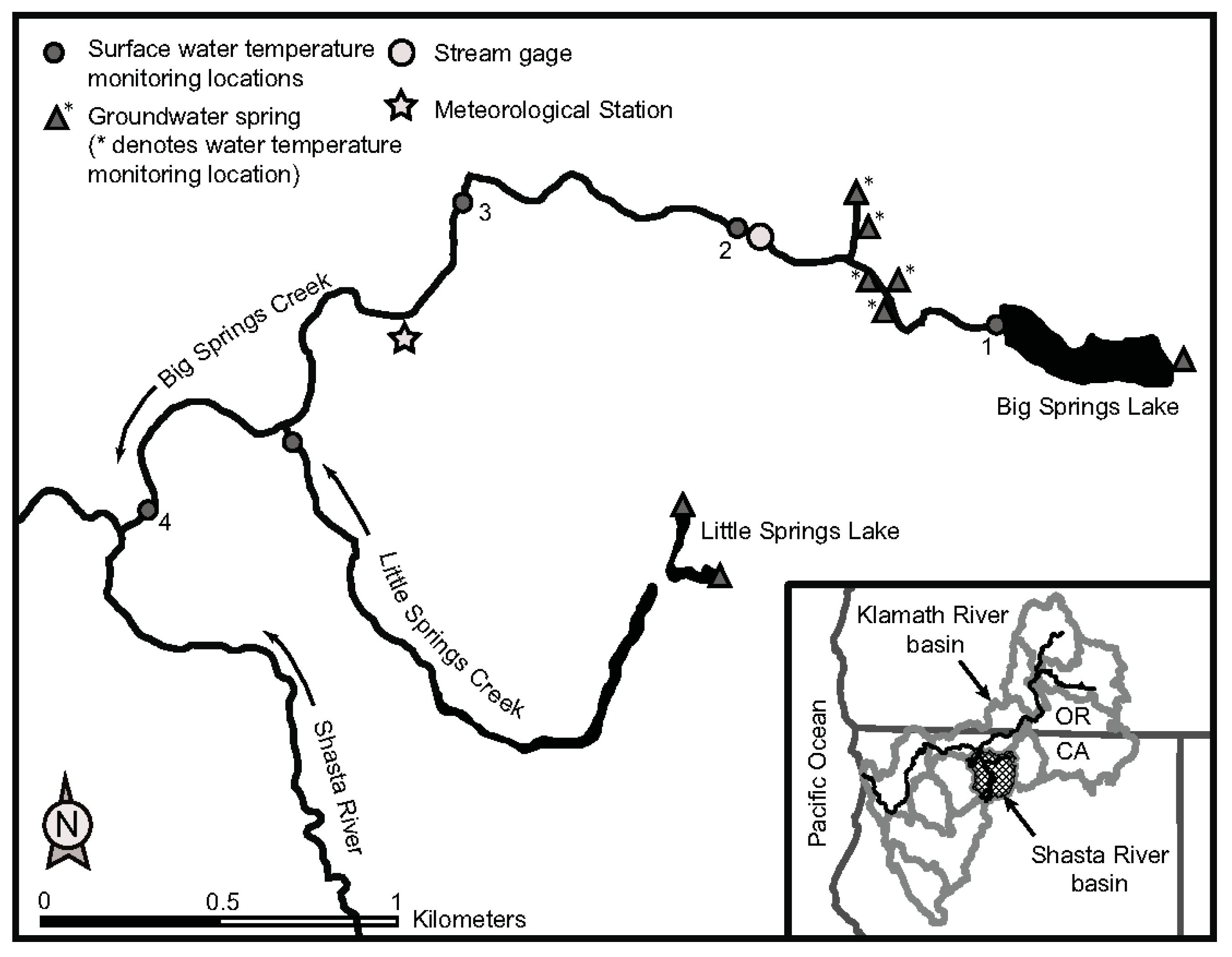
2.1. Study Site and Period

The study site included the 3.7 km reach of Big Springs Creek from the outlet of Big Springs Dam to the confluence with the Shasta River (Figure 1). The study period occurred between 1 April 2017 and 30 September 2017, during which the growing season coincided with the irrigation season on the ranches surrounding the creek. In addition, data were used from a previous flight in August 2015 to assess the spatial variability of interannual riverine canopy growth. Site access to the reach upstream from Site 2 (river kilometer (rkm) 2.7) extending to Site 1 (rkm 3.7) was limited to 1 day per month, with access dates negotiated with the landowner at least 6 weeks prior to the proposed sampling dates. Once agreed upon, access dates could not be rescheduled.

2.2. Riverine Canopy Surveys

Riverine canopy surveys were completed using a 3DR Solo Quadcopter, which was modified to attach a Canon Powershot S100 digital camera. A flight path of 84 north–south oriented transects covering 22.5 linear kilometers were flown from an altitude of 104 m, with a flight speed of 16 km per hour to achieve an approximate image side and end overlap of 70%. Control points were established at 36 locations by monumenting 13 cm2 bolts upside-down in concrete, then surveying the top of the bolt using a Topcon Hiper V Real Time Kinematic GPS unit with 5 mm horizontal and 10 mm vertical accuracy. Control point targets were created using 0.6 m2 wood boards that were painted white, then marked with 5 cm black lines across the diagonals, and finally had a 1.3 cm hole drilled in the center of the board. The targets were then mounted on the monumented bolts (targets were held in place using a washer and nut both above and below the board) to help visual identification of the control points in the UAV imagery. The camera was programmed to take images at a 5-s interval. Images were reviewed and adjusted for brightness, then stitched together using Agisoft Photoscan Professional (v 1.2.6, St. Petersburg, Russia). Completed Photoscan models were georeferenced by identifying the control point targets in the individual photos. Orthomosaic and digital elevation model (DEM) layers, each with a 0.05 m resolution, were then created and exported as georeferenced tiff files.
The spatial and temporal variability of riverine canopy growth was analyzed using supervised image classification and analysis of the tiff files in ArcMap 10.5 (Redlands, CA, USA). First, the orthomosaic image was clipped to include only the wetted channel. Also, polygons of a willow stand were made to mask the area from analysis of canopy extent due to aquatic macrophytes. Then, training samples of 40–50 merged polygons were created for each of two classes: open water and emergent aquatic vegetation. These training samples were then used to classify the clipped orthomosaic image of Big Springs Creek and to estimate the percent area covered by emergent aquatic vegetation. Misclassification was determined by extracting the classified image raster pixels in the training samples. Temporal changes were explored by comparing the percent area covered from one survey to the next during the 2017 monitoring period. Spatial changes were explored by comparing August surveys from 2015 and 2017, and analyzed to identify cover class areas that remained consistent.

2.3. Water Temperature Modeling

Once the temporal and spatial trends were analyzed, an existing hydrodynamic and water temperature model of Big Springs Creek [16] was used to simulate water temperature conditions given various frequencies of canopy growth interpolation. RMA-11 is a Fortran-based, proprietary model that has been applied in various water temperature studies [9,16,35]. Riverine canopy surveys were used to develop element classes in the unstructured grid that represented various amounts of canopy cover using numerical representations of shade and roughness; no other changes to the grid were made so as to test model performance due solely to refined aquatic vegetation data.
The cover in each element was determined by extracting the classified image raster pixels of each class (open and cover) for the area covered by the element and calculating the percent cover for each element at each of the four survey dates. Weekly changes in percent cover for each model element were determined using a linear interpolation between survey points. To simplify the computational requirements of the numerical water temperature model, element cover types were binned into classes representing no cover (0–10% covered areas in the classified images), 20% cover (10–30%), 40% cover (30–50%), 60% cover (50–70%), 80% cover (70–90%), and full cover (90–100% cover). A histogram of element classes was developed to review the trend of cover classes through the simulation period.
Shade for each element class was calculated by assigning the empirically observed solar radiation for covered areas (i.e., 12% of solar radiation was measured in covered areas [16]) to the proportion of the element that represented its cover class, plus full solar radiation to the remaining area Equation (1).
element shade = (percent cover × 0.12) + (percent open × 1)
Roughness for each element class was similarly calculated, using empirically-based values for this site [16] Equation (2):
element roughness = (percent cover × 0.31) + (percent open × 0.07)
The water temperature model was run for a continuous period between 1 June and 15 August to simulate three different time-step adjustments to the riverine canopy: weekly, bi-weekly and monthly. Shade and roughness values were updated to reflect new values at the start of each step, with no smoothing applied. Results of each simulation were analyzed at four locations (Figure 1) using mean bias, mean absolute error (MAE) and root mean square error (RMSE), keeping with performance criteria developed for management decision-making applications [16,32]. RMSE was particularly useful as it remains unbiased by seasonal cycles [9]; given the expected seasonal dynamics of canopy growth, controlling for seasonally-derived bias is a critical feature of this study.

3. Results

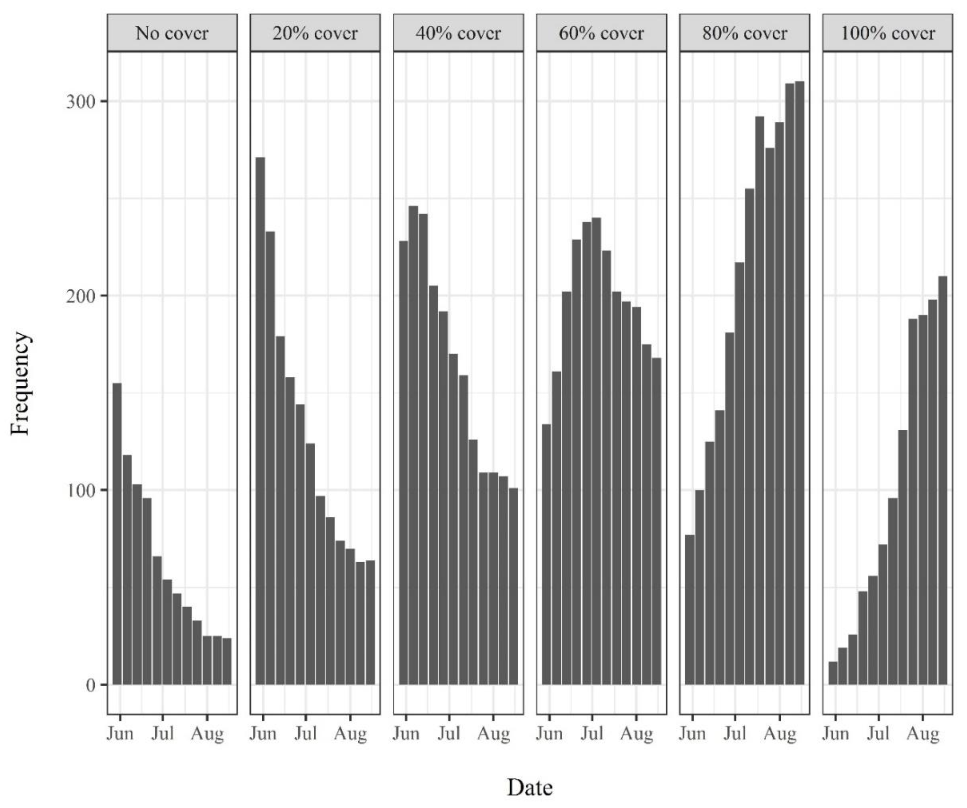
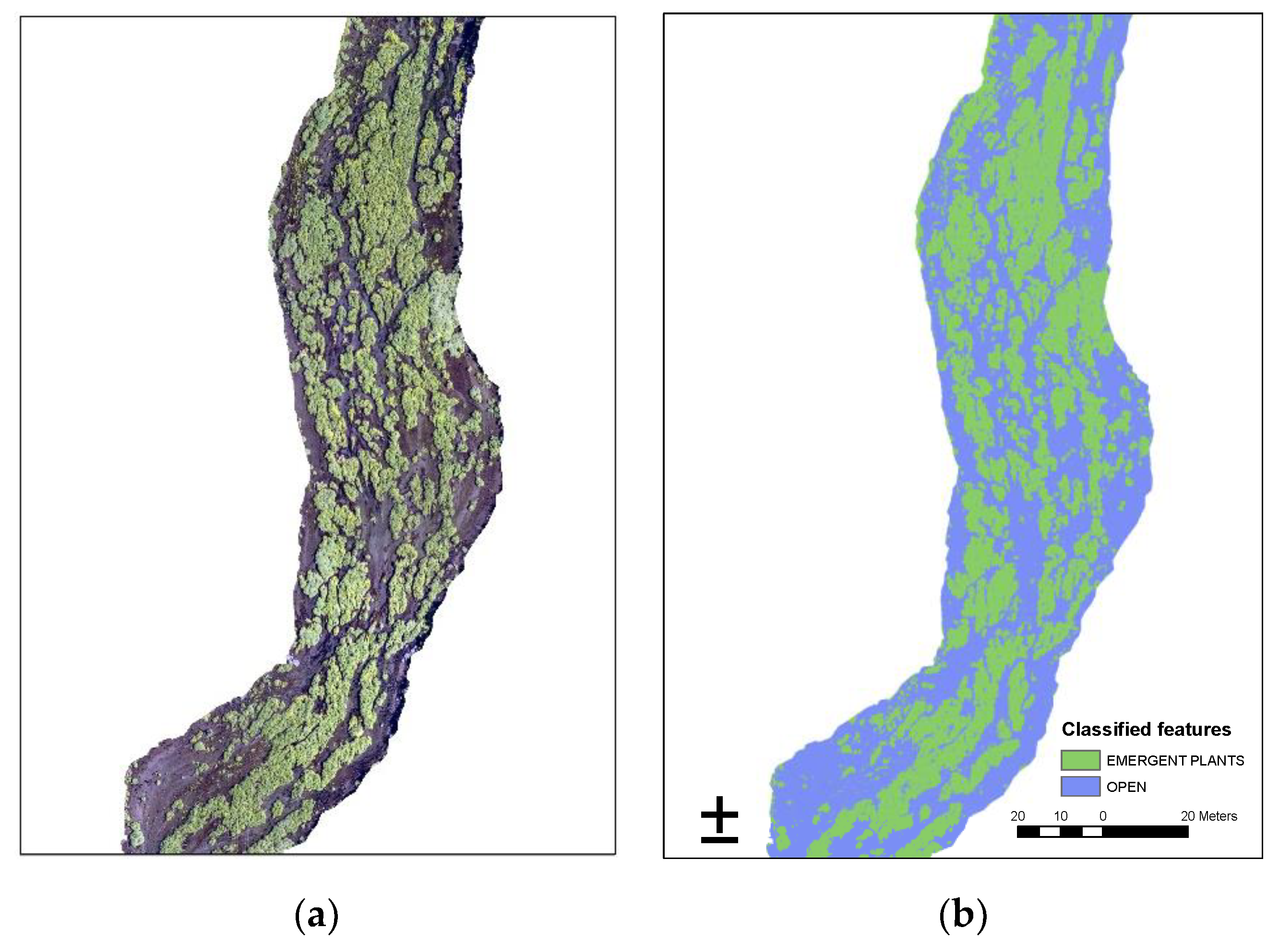
3.1. Riverine Canopy Surveys

Due to the long lead time necessary for scheduling access to the study site, field conditions were not always conducive to UAV flights. Inclement weather or wind speeds greater than 16 km per hour prevented riverine canopy surveys for the months of April and September. During the remaining visits, UAV flights of the entire reach were completed over 2 days (Table 1).
The supervised classification was able to distinguish between open channel and emergent plants (i.e., canopy) for all orthomosaic images produced via UAV monitoring (Figure 2). An analysis of misclassified pixels showed that the training samples were sufficient to classify cover type with 1.3% and 4.0% misclassification for open channel and emergent plant classes, respectively.
Canopy cover changed both temporally and spatially in Big Springs Creek. Temporally, cover increased from 38% in May 2017 to 74% in August 2017 (36% increase), with the largest change occurring between June and July (18% increase) and the smallest change occurring between July and August (4% increase) (Table 1). For the spatial analysis, differences in the flight path used in 2015 resulted in poor image resolution or lack of coverage at the margins of the orthomosaic. Thus, of the total area surveyed in 2017, 16% (25,989 m2) could not be compared to data from the 2015 flight. Of the remaining area, the cover remained consistent over 66% (108,352 m2) of the stream from August 2015 to August 2017, while 16% (26,765 m2) shifted from the canopy to open channel and 2% (3197 m2) shifted from the open channel to canopy (Table 2).

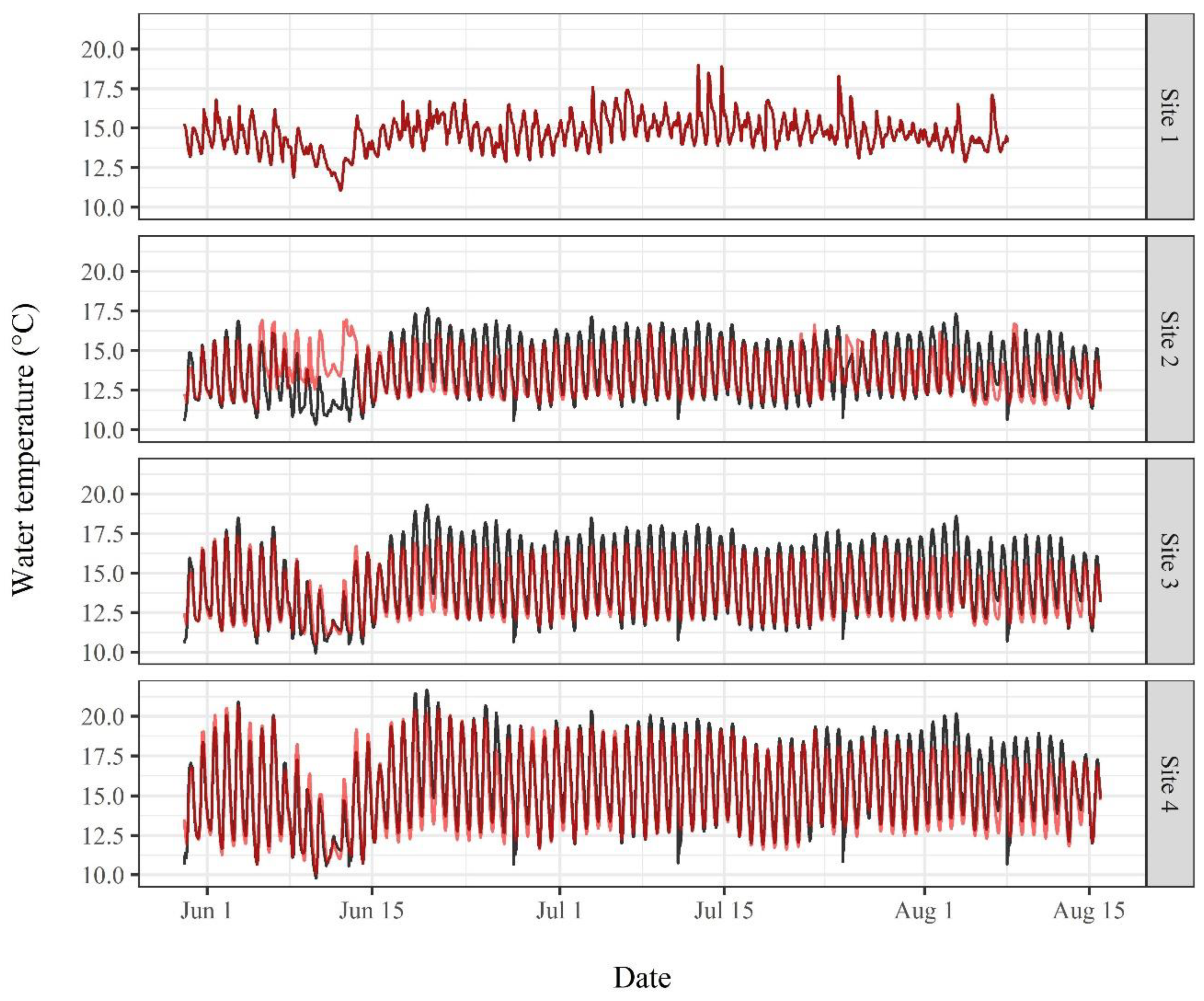
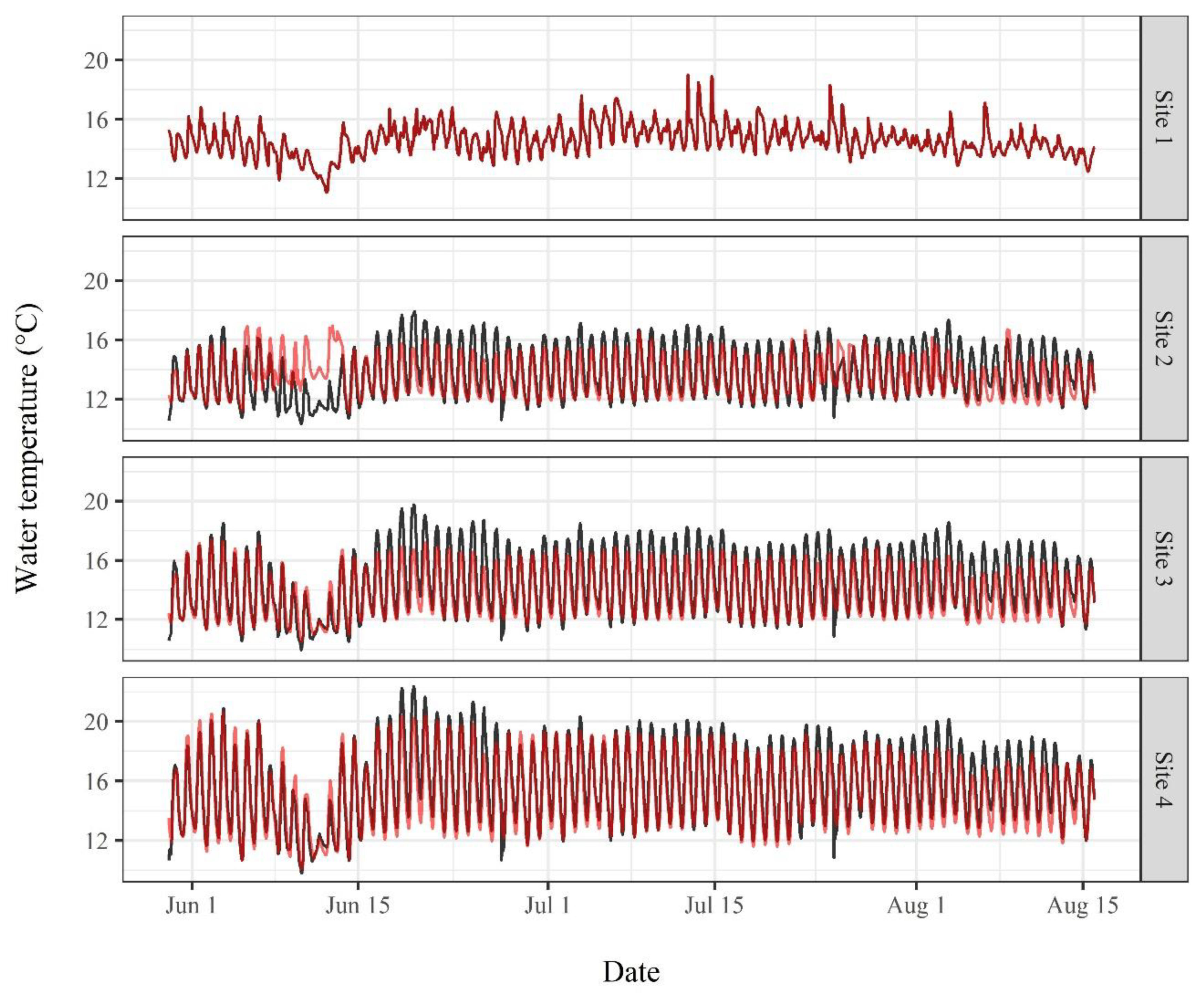
3.2. Water Temperature Modeling

The histogram of the element classes shows that during the beginning of the simulation period, element classes were dominated by areas with cover ≤40% (Figure 3). As the simulation period progressed, classes were dominated by areas with cover ≥60%. While most classes showed steady trends either increasing or decreasing their frequency, the element class that represented 60% cover initially occurred more frequently, then declined. From its peak frequency, the 60% coverage class saw a net 30% transition to greater coverage classes. The highest and lowest cover classes also showed indications of a plateau at the end of the modeled period, while areas in the 60% and 80% covered classes showed steady decreasing and increasing trends, respectfully.
Regardless of the frequency with which canopy growth was simulated, the water temperature model produced results that met the performance criteria (Table 3). Simulated water temperatures were generally warmer than observed water temperatures, as shown by the positive mean bias across all simulations. For all simulations, mean bias increased through location 3, then decreased towards the mouth, Site 4. This gradual increase in mean bias, then decline, suggests that better representation of local features such as groundwater inflow volumes may be necessary to apply the model for more refined management objectives. Mean absolute error (MAE) remained consistent at each site (with the expected exception of the boundary condition), showing no substantial changes in accuracy as the model progressed through the study area. Root mean squared error (RSME) also remained well within the 1.5*MAE threshold for all sites and simulations, indicating no anomalous, large errors.
A closer review of the modeled water temperatures compared to observed water temperatures show where the likely sources of error occurred. Given the comparable performance of each simulation, only plots for the weekly growth simulation are presented and discussed. Additional plots of the biweekly and monthly growth simulations are presented in Appendix A.
Though the performance metrics show a mean bias of up to 0.6 °C, the plots of modeled to observed water temperatures show that daily maximum water temperatures are generally overestimated while daily minimum water temperatures are well replicated (Figure 4). Site 1 represents a boundary condition of the model and is defined by the observed data at that site. At Sites 2 and 3, maximum water temperatures are generally over-estimated—a trend that remains consistent throughout the simulation period. At Site 2, observed water temperatures from 5 June to 13 June appear anomalous when compared to the other sites, suggesting that the observed data may not be an accurate record, contributing to the larger error at that site. By Site 4, the modeled diurnal water temperatures better match the observed record, with better agreement of both daily maximum and minimum water temperatures. However, agreement of modeled to observed daily maximum water temperatures declines towards the end of the simulation.
Sites 2–4 also show periodic underestimates of daily minimum water temperatures that occur coincidently with the shift in coverage represented in the model. Similar results are shown in the bi-weekly (Figure A1) and monthly (Figure A2) results. While the more frequent updates to canopy growth introduce more frequent errors for several hours after the new cover is introduced, results for the diurnal extremes (i.e., daily maximums and minimums) appear to be better simulated.

4. Discussion

As recently as the 1990s, local human activities were widely viewed as the dominant influence on thermal regimes in streams across the globe, rather than large-scale climate change [11]. By the early aughts, though, climate change was rapidly identified as a major driver of stream temperature changes [3]. While many management strategies focus on water quantity, the relationship between riparian canopies and climate change have long been recognized as issues of greater consequence to thermal regimes [11]. Results from this and previous studies suggest that riverine canopies may play a similarly influential relationship in mitigating the predicted effects of climate change [25]. The findings from this study have broader implications for three facets of water temperature management for cold-water ecosystems: extending canopy monitoring methodology, as shown by combining UAV and digital photography technology; the important role of riverine canopies in thermal regimes; and water temperature modeling for large-scale versus local management objectives.

4.1. UAV Survey Methods

The results of this study show that UAV survey methods provide an efficient approach (both in terms of equipment cost and person-time) to gather near-census data quantifying cover over a mid-sized stream. Prior to the use of UAVs for canopy cover monitoring, methods were limited by the spatial extent that could be covered due to most survey elevations, as well as the cost and time needed to perform the surveys. As recently as 2017, imagery taken from a height of 2–5 m above a stream’s water surface was considered aerial imagery [36,37]. Those survey altitude limits further constrained the size of stream that could be surveyed; at the upper bound of those aerial surveys, study sites were limited to streams up to 10 m wide [36]. This study shows how utilizing the flight ability of UAVs greatly expands the area that can be surveyed: in 2 days, full surveys of Big Springs Creek were completed, which covered 3.7 km and included stream reaches as wide as 300 m [34].
In addition, this study shows how digital photography methods used for low-elevation surveys can be extended by combining digital photography with UAV technology. Alternative methods that have been developed to assess cover, such as riparian surveys using canopy densitometers [38], are impractical for riverine canopies, where emergent plants grow through and remain near the water surface. Digital photography provides a cost-effective approach that has been previously utilized for aquatic plant mapping at lower elevations [36]; this study illustrates how similar methods are successful at higher survey elevations, extending this method to a wide range of stream sizes. Despite its classification as “low-spectral resolution,” the three-band (red-green-blue) survey was sufficient for classification accuracy, which makes this method a cost-effective alternative to others that use multi-spectral imaging.
Some limitations of this study can be overcome by standardizing the flight paths and survey extent of UAVs. A comparison of 2015 to 2017 data illustrated the need for wide spatial margins for survey areas, as well as the value in establishing repeatable flight paths to ensure reproducible and comparable survey areas. In addition, access limitations also highlighted how sites with more access flexibility are better suited to UAV monitoring, which requires dependable field conditions that typically are only well-forecast several days in advance. Finally, this method may benefit from additional ground truthing by manually surveying randomly selected in-stream areas using an RTK or other comparable methods.

4.2. Riverine Canopy Growth

Understanding the thermal regime processes that will buffer against predicted climate change is critical to conserving and managing cold-water ecosystems. The results of this study show that riverine canopy processes can be well-characterized using monthly datasets and how its influence in the thermal regime becomes stronger as the canopy more fully develops throughout the growing season. Early in the growing season, the riverine canopy is dominated by relatively low-coverage areas: This period coincides with previous observations of annual maximum water temperatures in thermal regimes controlled by riverine canopies [16], when fish like juvenile coho may be more vulnerable to elevated water temperatures [39]. Improving resolution around early season growth may be critical, as previous work has shown that water in and above submerged vegetation may be more sensitive to solar radiation than open-channel flow [40,41]. As such, additional management actions may be necessary to mediate annual maximum water temperatures during those early growth periods.
As the growing season progresses, there’s a transition across mid-coverage element areas as low-coverage areas become high coverage areas. Interestingly, lack of plateau in the 60% and 80% cover classes suggest that additional growth may be occurring and that the surveys completed in mid-August did not catch the transition from growth to senescence. Previous studies show that biomass continued to increase into September [16]. Extending the surveys later in the year would help quantify the peak coverage provided by the riverine canopy, as well as the timing of when the canopy begins to senesce. As well as extending the data describing the seasonal trends of canopy growth, additional data to quantify the shade provided by the canopy would further improve understanding of those thermal regimes. As warm temperatures and dry conditions extend later into the year [42], understanding the full potential of the riverine canopy to act as a buffer against these conditions is critical to understanding the potential management challenges for thermally-sensitive ecosystems.
Once the riverine canopy transitions into predominately fuller coverage, its advantages over riparian shade as a solar radiation buffer are clear. Riparian shade needs both longer time frames and spatial scales to achieve similar effectiveness to riverine canopies [16,17]. Tree height and shape, channel width and shape (i.e., straight or meandering), and channel orientation are all factors that limit the effectiveness of riparian shade [14,25]; riverine canopies have no limitations analogous to these riparian features. Despite these drawbacks of riparian canopies, research into the relationship between riparian cover and stream temperatures suggests useful considerations for future work. Microclimate changes due to extensive cover may shift energy fluxes in the heat budget and fluxes that are generally negligible in less densely covered reaches may become more influential in the overall thermal regime [14,43]. Examining the effects of canopy-controlled thermal regimes should include an analysis of daily extreme (i.e., maximum and minimum) water temperatures to ensure that sufficient minimum temperature conditions are maintained in streams targeted for salmonid or other cold-water species recovery. Also, the ability of aquatic plants to colonize 70% of the channel is consistent with the findings of other riparian studies for the cover extent needed to affect both temperature control [14,18] and macroinvertebrate recovery [18]. Those findings are confirmed by the results of this and previous studies, which show that seasonal water temperatures in Big Springs Creek begin to cool in late June/early July [16], when the riverine canopy covers nearly 70% of the stream surface.
Given the larger stream-orders that may be affected by riverine canopies, vs. riparian, it would be useful to determine the geographic extent of these types of streams, as restoration of the riverine canopy process could influence water temperatures on the reach-scale [34,44] and mitigate for climate change [25]. On a reach-scale, regression equations have been used to identify predictor variables for water temperature, such as riparian vegetation [15], and could be useful tools to explore whether the riverine canopy-controlled thermal regime is representative of a class of rivers. Such findings could have important implications for mitigating the effects of climate change, as canopy-controlled thermal regimes may result in cooler stream temperatures than currently observed in spite of predicted climate warming [14,25]. In addition, while this study focuses on the relationship between riverine canopies and thermal regimes, other studies have shown strong relationships between aquatic plants and channel hydraulics [45,46,47]. However, because aquatic plants senesce each year, the role of riverine canopies and their seasonal effects on physical salmonid habitat, and, by extension, salmonid life history strategies, may show an interesting contrast to studies that focus on large woody debris and other semi-permanent features for cover and velocity utilization by juvenile coho [48,49].

4.3. Water Temperature Modeling

Finally, water temperature modeling is used to transform improved monitoring using UAV technology and the improved understanding of the role riverine canopies play in the thermal regime into a potential management tool. While model results show that monthly interpolated canopy growth is sufficient to model water temperatures, the performance metrics and comparative plots suggest that there is additional room for improvement. The negligible improvement that followed more refined temporal resolution of canopy growth suggests that further improvement is more likely to result from better representation of other processes in the thermal regime. Such processes include better representation of substantial groundwater inflows to the creek, both in the overall quantity and distribution of flows among discrete groundwater sources. Due to the dominant role that groundwater plays in spring-fed stream thermal regimes [50,51], additional work is recommended to improve the understanding of the conductive and advective heat flux through the stream bed. Such work would also help clarify the issue of potential shifts in dominant heat flux processes given the microclimate effects of canopy cover. Also, the model showed some short-term (e.g., over a period of hours) sensitivity to the periodic update of canopy cover, and could benefit from additional refinement such as transitional smoothing between cover configurations. As such, the model is better suited for large-scale management objectives (e.g., managing water temperature conditions that are exported to the reach-scale habitat in the downstream Shasta River), but requires refinement before it could be confidently applied to managing the local habitat within Big Springs Creek.
Additional work that explores model performance in response to more refined grid structures would help illustrate the balance between computational efficiency and the data required to accurately simulate the heat exchange processes dictated by the riverine canopy. Models developed at fine spatial scales can be particularly useful for understanding the relationship between ecosystem dynamics and water temperature processes [9]. Also, while the decision to use a proprietary model was influenced by considerable investments made in previous stages of this research, publicly available models would allow for more transparency. Future stages, particularly those with the objective of evaluating management decisions, should weigh the benefit of using currently available models against the desirability for more transparent, and potentially transferable, modeling methods.
Water resource and fisheries managers need to make decisions based on the thermal regime of a stream [19], which may be controlled by factors other than stream flow or air temperature. In these cases, deterministic modeling may be necessary when longer-term datasets are unavailable, particularly where novel thermal processes have been identified. Future studies may want to explore statistical relationships between riverine cover and stream temperature to develop management tools that are less data-intensive than deterministic models.

Author Contributions

Conceptualization, A.W. and E.H.; Methodology, A.W. and E.H.; Software, A.W. and E.H.; Validation, A.W. and E.H.; Formal Analysis, A.W. and E.H.; Investigation, A.W. and E.H.; Resources, A.W. and E.H.; Data Curation, A.W. and E.H.; Writing-Original Draft Preparation, A.W. and E.H.; Writing-Review & Editing, A.W.; Visualization, A.W. and E.H; Supervision, A.W.; Project Administration, A.W.

Funding

This research received no external funding.

Acknowledgments

We’d like to thank the Nature Conservancy and Irene Busk for providing access to their properties and permission to use the study site; Devon Lambert for his considerable field assistance; Ian King for his willingness to answer questions about implementing RMA; Sarah Yarnell for donating her UAV equipment for the surveys; and Carson Jeffres for his willingness to let E.H. volunteer time and expertise for this study in addition to his valuable role in other projects. We’d also like to thank two anonymous reviewers for their thoughtful and detailed reviews, which considerably improved this manuscript.

Conflicts of Interest

The authors declare no conflict of interest.

Appendix A

Figure A1. Plots of the modeled (black line) water temperature versus observed (red line) water temperatures for the biweekly canopy growth simulation.
Hydrology 06 00006 g0a1
Figure A2. Plots of the modeled (black line) water temperature versus observed (red line) water temperatures for the monthly canopy growth simulation.
Hydrology 06 00006 g0a2

References

  1. Caissie, D. The thermal regime of rivers: A review. Freshw. Biol. 2006, 51, 1389–1406. [Google Scholar] [CrossRef]
  2. Steel, E.A.; Beechie, T.J.; Torgersen, C.E.; Fullerton, A.H. Envisioning, quantifying, and managing thermal regimes on river networks. BioScience 2017, 67, 506–522. [Google Scholar] [CrossRef]
  3. Webb, B.W.; Hannah, D.M.; Moore, R.D.; Brown, L.E.; Nobilis, F. Recent advances in stream and river temperature research. Hydrol. Process. 2008, 22, 902–918. [Google Scholar] [CrossRef]
  4. Davis, J.; Baxter, C.; Rosi-Marshall, E.; Pierce, J.; Crosby, B. Anticipating stream ecosystem responses to climate change: Toward predictions that incorporate effects via land–water linkages. Ecosystems 2013, 16, 909–922. [Google Scholar] [CrossRef]
  5. Woodward, G.; Perkins, D.M.; Brown, L.E. Climate change and freshwater ecosystems: Impacts across multiple levels of organization. Philos. Trans. R. Soc. Lond. B Biol. Sci. 2010, 365, 2093–2106. [Google Scholar] [CrossRef] [PubMed]
  6. Harper, M.P.; Peckarsky, B.L. Emergence cues of a mayfly in a high-altitude stream ecosystem: Potential response to climate change. Ecol. Appl. 2006, 16, 612–621. [Google Scholar] [CrossRef]
  7. Isaak, D.J.; Wenger, S.J.; Young, M.K. Big biology meets microclimatology: Defining thermal niches of ectotherms at landscape scales for conservation planning. Ecol. Appl. 2017, 27, 977–990. [Google Scholar] [CrossRef]
  8. Isaak, D.J.; Wenger, S.J.; Peterson, E.E.; Ver Hoef, J.M.; Nagel, D.E.; Luce, C.H.; Hostetler, S.W.; Dunham, J.B.; Roper, B.B.; Wollrab, S.P. The NorWEST summer stream temperature model and scenarios for the western U.S.: A crowd-sourced database and new geospatial tools foster a user community and predict broad climate warming of rivers and streams. Water Resour. Res. 2017, 53, 9181–9205. [Google Scholar] [CrossRef]
  9. Dugdale, S.J.; Hannah, D.M.; Malcolm, I.A. River temperature modelling: A review of process-based approaches and future directions. Earth Sci. Rev. 2017, 175, 87–113. [Google Scholar] [CrossRef]
  10. Hannah, D.M.; Garner, G. River water temperature in the United Kingdom: Changes over the 20th century and possible changes over the 21st century. Prog. Phys. Geogr. 2015, 39, 68–92. [Google Scholar] [CrossRef] [Green Version]
  11. Webb, B. Trends in stream and river temperature. Hydrol. Process. 1996, 10, 205–226. [Google Scholar] [CrossRef]
  12. Moore, R.D. Stream temperature patterns in British Columbia, Canada, based on routine spot measurements. Can. Water Resour. J. 2006, 31, 41–56. [Google Scholar] [CrossRef]
  13. Johnson, S.L. Factors influencing stream temperatures in small streams: Substrate effects and a shading experiment. Can. J. Fish. Aquat. Sci. 2004, 61, 913–923. [Google Scholar] [CrossRef]
  14. Garner, G.; Malcolm, I.A.; Sadler, J.P.; Hannah, D.M. The role of riparian vegetation density, channel orientation and water velocity in determining river temperature dynamics. J. Hydrol. 2017, 553, 471–485. [Google Scholar] [CrossRef]
  15. Moore, R.; Spittlehouse, D.; Story, A. Riparian microclimate and stream temperature response to forest harvesting: A review 1. JAWRA J. Am. Water Resour. Assoc. 2005, 41, 813–834. [Google Scholar] [CrossRef]
  16. Willis, A.D.; Nichols, A.L.; Holmes, E.J.; Jeffres, C.A.; Fowler, A.C.; Babcock, C.A.; Deas, M.L. Seasonal aquatic macrophytes reduce water temperatures via a riverine canopy in a spring-fed stream. Freshw. Sci. 2017, 36, 508–522. [Google Scholar] [CrossRef]
  17. Kalny, G.; Laaha, G.; Melcher, A.; Trimmel, H.; Weihs, P.; Rauch, H.P. The influence of riparian vegetation shading on water temperature during low flow conditions in a medium sized river. Knowl. Manag. Aquat. Ecosyst. 2017, 418, 5. [Google Scholar] [CrossRef]
  18. Rutherford, C.J.; Meleason, M.A.; Davies-Colley, R.J. Modelling stream shade: 2. Predicting the effects of canopy shape and changes over time. Ecol. Eng. 2018, 120, 487–496. [Google Scholar] [CrossRef]
  19. Sinokrot, B.A.; Stefan, H.G. Stream temperature dynamics: Measurements and modeling. Water Resour. Res. 1993, 29, 2299–2312. [Google Scholar] [CrossRef]
  20. Benyahya, L.; Caissie, D.; St-Hilaire, A.; Ouarda, T.B.; Bobée, B. A review of statistical water temperature models. Can. Water Resour. J. 2007, 32, 179–192. [Google Scholar] [CrossRef]
  21. Schabenberger, O.; Gotway, C.A. Statistical Methods for Spatial Data Analysis; CRC Press: Boca Raton, FL, USA, 2017. [Google Scholar]
  22. Trimmel, H.; Weihs, P.; Leidinger, D.; Formayer, H.; Kalny, G.; Melcher, A. Can riparian vegetation shade mitigate the expected rise in stream temperatures due to climate change during heat waves in a human-impacted pre-alpine river? Hydrol. Earth Syst. Sci. 2018, 22, 437–461. [Google Scholar] [CrossRef] [Green Version]
  23. Loicq, P.; Moatar, F.; Jullian, Y.; Dugdale, S.J.; Hannah, D.M. Improving representation of riparian vegetation shading in a regional stream temperature model using lidar data. Sci. Total Environ. 2018, 624, 480–490. [Google Scholar] [CrossRef] [PubMed]
  24. McGrath, E.; Neumann, N.; Nichol, C. A statistical model for managing water temperature in streams with anthropogenic influences. River Res. Appl. 2017, 33, 123–134. [Google Scholar] [CrossRef]
  25. Wondzell, S.M.; Diabat, M.; Haggerty, R. What matters most: Are future stream temperatures more sensitive to changing air temperatures, discharge, or riparian vegetation? JAWRA J. Am. Water Resour. Assoc. 2018. [Google Scholar] [CrossRef]
  26. Van Vliet, M.; Ludwig, F.; Zwolsman, J.; Weedon, G.; Kabat, P. Global river temperatures and sensitivity to atmospheric warming and changes in river flow. Water Resour. Res. 2011, 47. [Google Scholar] [CrossRef]
  27. Arora, R.; Tockner, K.; Venohr, M. Changing river temperatures in northern Germany: Trends and drivers of change. Hydrol. Process. 2016, 30, 3084–3096. [Google Scholar] [CrossRef]
  28. Ptak, M.; Choiński, A.; Kirviel, J. Long-term water temperature fluctuations in coastal rivers (southern Baltic) in Poland. Bull. Geogr. Phys. Geogr. Ser. 2016, 11, 35–42. [Google Scholar] [CrossRef] [Green Version]
  29. Null, S.E.; Viers, J.H.; Deas, M.L.; Tanaka, S.K.; Mount, J.F. Stream temperature sensitivity to climate warming in California’s Sierra Nevada: Impacts to coldwater habitat. Clim. Chang. 2013, 116, 149–170. [Google Scholar] [CrossRef]
  30. Moyle, P.B.; Lusardi, R.A.; Samuel, P.; Katz, J. State of the Salmonids: Status of Ccalifornia’s Emblematic Fishes 2017; University of California: Davis, CA, USA, 2017; p. 579. [Google Scholar]
  31. Vasseur, D.A.; DeLong, J.P.; Gilbert, B.; Greig, H.S.; Harley, C.D.; McCann, K.S.; Savage, V.; Tunney, T.D.; O’Connor, M.I. Increased temperature variation poses a greater risk to species than climate warming. Proc. R. Soc. Lond. B Biol. Sci. 2014, 281, 20132612. [Google Scholar] [CrossRef]
  32. Null, S.E.; Deas, M.L.; Lund, J.R. Flow and water temperature simulation for habitat restoration in the Shasta River, California. River Res. Appl. 2010, 26, 663–681. [Google Scholar] [CrossRef]
  33. Willis, A.D.; Campbell, A.M.; Fowler, A.C.; Babcock, C.A.; Howard, J.K.; Deas, M.L.; Nichols, A.L. Instream flows: New tools to quantify water quality conditions for returning adult Chinook salmon. J. Water Resour. Plan. Manag. 2015, 04015056. [Google Scholar] [CrossRef]
  34. Nichols, A.L.; Willis, A.D.; Jeffres, C.A.; Deas, M.L. Water temperature patterns below large groundwater springs: Management implications for coho salmon in the Shasta River, California. River Res. Appl. 2014, 30, 442–455. [Google Scholar] [CrossRef]
  35. Lowney, C.L. Stream temperature variation in regulated rivers: Evidence for a spatial pattern in daily minimum and maximum magnitudes. Water Resour. Res. 2000, 36, 2947–2955. [Google Scholar] [CrossRef] [Green Version]
  36. Verschoren, V.; Schoelynck, J.; Buis, K.; Visser, F.; Meire, P.; Temmerman, S. Mapping the spatio-temporal distribution of key vegetation cover properties in lowland river reaches, using digital photography. Environ. Monit. Assess. 2017, 189, 294. [Google Scholar] [CrossRef] [PubMed]
  37. Clark, P.E.; Johnson, D.E.; Hardegree, S.P. A direct approach for quantifying stream shading. Rangel. Ecol. Manag. 2008, 61, 339–345. [Google Scholar] [CrossRef]
  38. Kelley, C.E.; Krueger, W.C. Canopy cover and shade determinations in riparian zones 1. JAWRA J. Am. Water Resour. Assoc. 2005, 41, 37–046. [Google Scholar] [CrossRef]
  39. Richter, A.; Kolmes, S.A. Maximum temperature limits for chinook, coho, and chum salmon, and steelhead trout in the Pacific Northwest. Rev. Fish. Sci. 2005, 13, 23–49. [Google Scholar] [CrossRef]
  40. Rutherford, J.C.; Macaskill, J.B.; Williams, B.L. Natural water temperature variations in the lower Waikato River, New Zealand. N. Z. J. Mar. Freshw. Res. 1993, 27, 71–85. [Google Scholar] [CrossRef] [Green Version]
  41. Clark, E.; Webb, B.; Ladle, M. Microthermal gradients and ecological implications in Dorset rivers. Hydrol. Process. 1999, 13, 423–438. [Google Scholar] [CrossRef]
  42. Leung, L.R.; Qian, Y.; Bian, X.; Washington, W.M.; Han, J.; Roads, J.O. Mid-century ensemble regional climate change scenarios for the western United States. Clim. Chang. 2004, 62, 75–113. [Google Scholar] [CrossRef]
  43. Fabris, L.; Malcolm, I.A.; Buddendorf, W.B.; Soulsby, C. Integrating process-based flow and temperature models to assess riparian forests and temperature amelioration in salmon streams. Hydrol. Process. 2018, 32, 776–791. [Google Scholar] [CrossRef]
  44. Bartholow, J. Estimating cumulative effects of clearcutting on stream temperatures. Rivers 2000, 7, 284–297. [Google Scholar]
  45. Bal, K.; Struyf, E.; Vereecken, H.; Viaene, P.; De Doncker, L.; de Deckere, E.; Mostaert, F.; Meire, P. How do macrophyte distribution patterns affect hydraulic resistances? Ecol. Eng. 2011, 37, 529–533. [Google Scholar] [CrossRef]
  46. O’Hare, J.; O’Hare, M.; Gurnell, A.; Dunbar, M.; Scarlett, P.; Laize, C. Physical constraints on the distribution of macrophytes linked with flow and sediment dynamics in british rivers. River Res. Appl. 2011, 27, 671–683. [Google Scholar] [CrossRef]
  47. Green, J.C. Velocity and turbulence distribution around lotic macrophytes. Aquat. Ecol. 2005, 39, 1–10. [Google Scholar] [CrossRef]
  48. Lacey, R.J.; Millar, R.G. Reach scale hydraulic assessment of instream salmonid habitat restoration 1. JAWRA J. Am. Water Resour. Assoc. 2004, 40, 1631–1644. [Google Scholar] [CrossRef]
  49. McMahon, T.E.; Hartman, G.F. Influence of cover complexity and current velocity on winter habitat use by juvenile coho salmon (oncorhynchus kisutch). Can. J. Fish. Aquat. Sci. 1989, 46, 1551–1557. [Google Scholar] [CrossRef]
  50. Kurylyk, B.L.; Moore, R.D.; MacQuarrie, K.T. Scientific briefing: Quantifying streambed heat advection associated with groundwater–surface water interactions. Hydrol. Process. 2016, 30, 987–992. [Google Scholar] [CrossRef]
  51. Caissie, D.; Luce, C.H. Quantifying streambed advection and conduction heat fluxes. Water Resour. Res. 2017, 53, 1595–1624. [Google Scholar] [CrossRef]
Figure 1. A map of the study area. Sites 1–4 were used to test water temperature modeling performance. Approximate centroid UTM coordinates are 10T 547,987.38 m E, 4,605,393.41 m N.
Hydrology 06 00006 g001
Figure 2. An example of the (a) orthoimagery; (b) results of the supervised classification, using data gathered during Survey 2 in June 2017.
Hydrology 06 00006 g002
Figure 3. The distribution of element cover classes through the model simulation period.
Hydrology 06 00006 g003
Figure 4. Plots of the modeled (black line) water temperature versus observed (red line) water temperatures for the weekly canopy growth simulation.
Hydrology 06 00006 g004
Table 1. A summary of the survey dates and percent cover of Big Springs Creek.
SurveyFlight DatesCanopy Cover (%)Canopy Cover (m2)
Survey 122–23 May 20173861,668
Survey 219–20 June 20175387,776
Survey 323–24 July 201771117,348
Survey 415–16 August 201774121,583
Table 2. A summary of the percent area that shifted cover classes from August 2015 to August 2017.
Class ChangeArea (m2)Area (%)
Canopy to open channel25,98916
Open channel to canopy31972
No change108,35266
Area not analyzed26,76516
Table 3. A summary of performance results for each simulation of water temperatures given various frequencies of interpolated canopy growth. All performance metrics are measured in °C.
SiteRiver KilometerWeekly GrowthBiweekly GrowthMonthly Growth
(rkm)Mean BiasMAE bRMSE cMean BiasMAERMSEMean BiasMAERMSE
1 a3.70.00.00.00.00.00.00.00.00.0
22.60.30.91.20.30.91.10.40.91.2
31.70.60.81.00.70.81.00.70.91.1
40.00.30.70.90.40.70.80.50.70.9
a Boundary condition; b Mean absolute error; c Root mean square error.

