Modeling Water Quality Parameters Using Data-Driven Models, a Case Study Abu-Ziriq Marsh in South of Iraq

Abstract

Total dissolved solids (TDS) and electrical conductivity (EC) are important parameters in determining water quality for drinking and agricultural water, since they are directly associated to the concentration of salt in water and, hence, high values of these parameters cause low water quality indices. In addition, they play a significant role in hydrous life, effective water resources management and health studies. Thus, it is of critical importance to identify the optimum modeling method that would be capable to capture the behavior of these parameters. The aim of this study was to assess the ability of using three different models of artificial intelligence techniques: Adaptive neural based fuzzy inference system (ANFIS), artificial neural networks (ANNs) and Multiple Regression Model (MLR) to predict and estimate TDS and EC in Abu-Ziriq marsh south of Iraq. As so, eighty four monthly TDS and EC values collected from 2009 to 2018 were used in the evaluation. The collected data was randomly split into 75% for training and 25% for testing. The most effective input parameters to model TDS and EC were determined based on cross-correlation test. The three performance criteria: correlation coefficient (CC), root mean square error (RMSE) and Nash–Sutcliffe efficiency coefficient (NSE) were used to evaluate the performance of the developed models. It was found that nitrate (NO₃), calcium (Ca⁺²), magnesium (Mg⁺²), total hardness (T.H), sulfate (SO₄) and chloride (Cl⁻¹) are the most influential inputs on TDS. While calcium (Ca⁺²), magnesium (Mg⁺²), total hardness (T.H), sulfate (SO₄) and chloride (Cl⁻¹) are the most effective on EC. The comparison of the results showed that the three models can satisfactorily estimate the total dissolved solids and electrical conductivity, but ANFIS model outperformed the ANN and MLR models in the three performance criteria: RMSE, CC and NSE during the calibration and validation periods in modeling the two water quality parameters. ANFIS is recommended to be used as a predictive model for TDS and EC in the Iraqi marshes.

1. Introduction

Preserving water quality has become an urgent issue since it affects human health and hydrous ecosystems. With the continuous increase in population, there is an increasing need for water resources. Contamination of water sources resulting from some natural processes, including air inputs or climatic conditions, and through human pollutants such as non-treatment of sewage discharge and industrial activities, which might add further stress to water quality [1]. The considered important indicators of water quality are the electrical conductivity (EC) and the total dissolved solids (TDS). High values of these parameters cause low water quality because they are directly related to the concentration of salt in water. However, the direct estimations of EC and TDS are costly and take a long time [2]. Therefore, convenient, cost-effective, fast and reliable methods are needed for their estimations and prediction [3]. Though there are other feasible water quality parameters which could be of interest to be evaluated such as DO, BOD, or PH, but however, these parameters are essentially influenced by EC and TDS [4].

Recently, the use of data-driven models, such as adaptive neural-based fuzzy inference system (ANFIS), artificial neural networks (ANNs) and gene expression programming (GEP) have become viable alternative in most studies [5,6,7,8,9]. Artificial intelligence (AI) has been used in many water-related studies for example, water quality modeling and water management applications [3,10,11,12,13,14,15,16,17,18,19]. However, there are many other models reported in the literature such as The Soil and Water Assessment Tool (SWAT), Water Quality Analysis Simulation Program (WASP), A Modeling Framework for Simulating River and Stream Water Quality (QUALs) and MIKE 11 [2,20]. The advantages of adopting the AI techniques over others arise from their ability to self-learning from the data and hence minimizing error [1].

Tutmez et al. developed the ANFIS model to estimate electrical conductivity in ground water. It was shown that the ANFIS model outperforms the traditional methods in modeling EC based on TDS in the water [21]. Singh et al. used two ANNs models for computing the dissolved oxygen (DO) and biochemical oxygen demand (BOD) levels of the Gomti river in India. In their study, 11 parameters were used as input variables and two variables as output at the Gomti River. The result showed that the ANN model can be used successfully in estimating water quality parameters [22]. Kisi and Murat used the ANFIS and radial basis neural network (RBN) models to predict DO values by using different input parameters, including discharge, pH, and temperature and EC at Fountain Creek Stream-Gauging Station, which covers 9 years of daily data. The results showed the RBNN model was better than ANFIS model in the prediction of DO values [18]. Wen et al. developed ANN model to estimate the DO values of Heihe River in northwestern China. The input parameters of the neural network were EC, PH, total hardness, chloride (Cl⁻¹), total hardness, calcium (Ca⁺²), total alkalinity, nitrate nitrogen (NO₃-N), and ammoniacal nitrogen (NH₄-N) with one output DO. The result indicated that the ANN model can be used successfully to estimate DO concentrations [23]. Montaseri et al. used three AI approaches, namely ANN, two different ANFIS including ANFIS with grid partition (ANFIS-GP) and ANFIS with subtractive clustering (ANFIS-SC), GEP, wavelet-ANN, wavelet-ANFIS and wavelet-GEP in predicting TDS at Nazlu Chay (northwest of Iran), Tajan (north of Iran), Zayandeh Rud (central of Iran) and Helleh (south of Iran) basins over a period of 20 years. EC, Na and Cl parameters were selected as input variables to forecast amount of TDS. A comparison of the results in this study showed that the performance of the wavelet-GEP was superior to the other AI models applied in TDS prediction for all basins [24]. Orouji et al. utilized the ANFIS and genetic programming (GP) as two data-driven models to predict and simulate water quality parameters (i.e., EC and TDS) of the Astane station in Sefidrood River, Iran. Both models of the data-driven succeeded in determining the water quality parameters [25]. Ay and Kişi used ANN, radial basis neural network, and two different ANFIS to estimation DO concentration. Moreover, the estimations of these models are compared with the multiple linear regressions. In this context, monthly mean quantities of the temperature, pH, EC, discharge and DO are used in modeling at Broad River near Carlisle, USA. The accuracy of the models is compared with one other by using determination coefficient, mean absolute error, root mean square error and mean absolute relative error statistics. Results indicate that radial basis neural network method performs better than the other methods in modeling monthly mean dissolved oxygen concentration [26]. Ghavidel used four AI approaches, namely two ANFIS including ANFIS-GP and ANFIS with subtractive clustering (ANFIS-SC), ANN and GEP for the estimation of TDS in the Zarinehroud basin in northwest of Iran. The result indicated that the GEP can be used successfully over than other data-driven models [10]. Edwin et al. explored the ability of ANN to predict dissolved oxygen in Lake Victoria basin, Kenya. Four input variables of temperature, turbidity, pH and EC were used. The data consisted of 113 monthly values for the input variables and output variable from 2009–2013 which were split into training and testing datasets. The results obtained during training and testing revealed that the ANN could be used as a monitoring tool in the prediction of dissolved oxygen. Obviously, there is no specific method attained a universal acceptance in terms of its applicability, therefore, further evaluation is needed based on data specific area [17].

The main objective of this study is to identify the optimum model, which could be used to model the water quality parameters in Abu-Ziriq marsh south of Iraq. Thence, three different algorithms (i.e., ANFIS, ANN and MLR) methods were investigated to model both water quality parameters such as TDS and EC. It is known that the direct and indirect measuring of EC and TDS values is expensive in Iraq. Therefore, the development of a model with a minimal number of chemical parameters but with acceptable accuracy to estimate EC and TDS values reduces the cost of water quality monitoring.

The study area was selected based on its importance in terms of the amount of inflow water; representing a good example of the ecological system; and its role in the Iraqi marshes revives. The cross correlation (Pearson correlation) was employed to select the best-input parameters with a significant level of 0.01. The models were assessed based on three evaluation criteria, which are correlation coefficient, root mean square error, and Nash and Sutcliff coefficient efficiency.

2. Materials and Methods

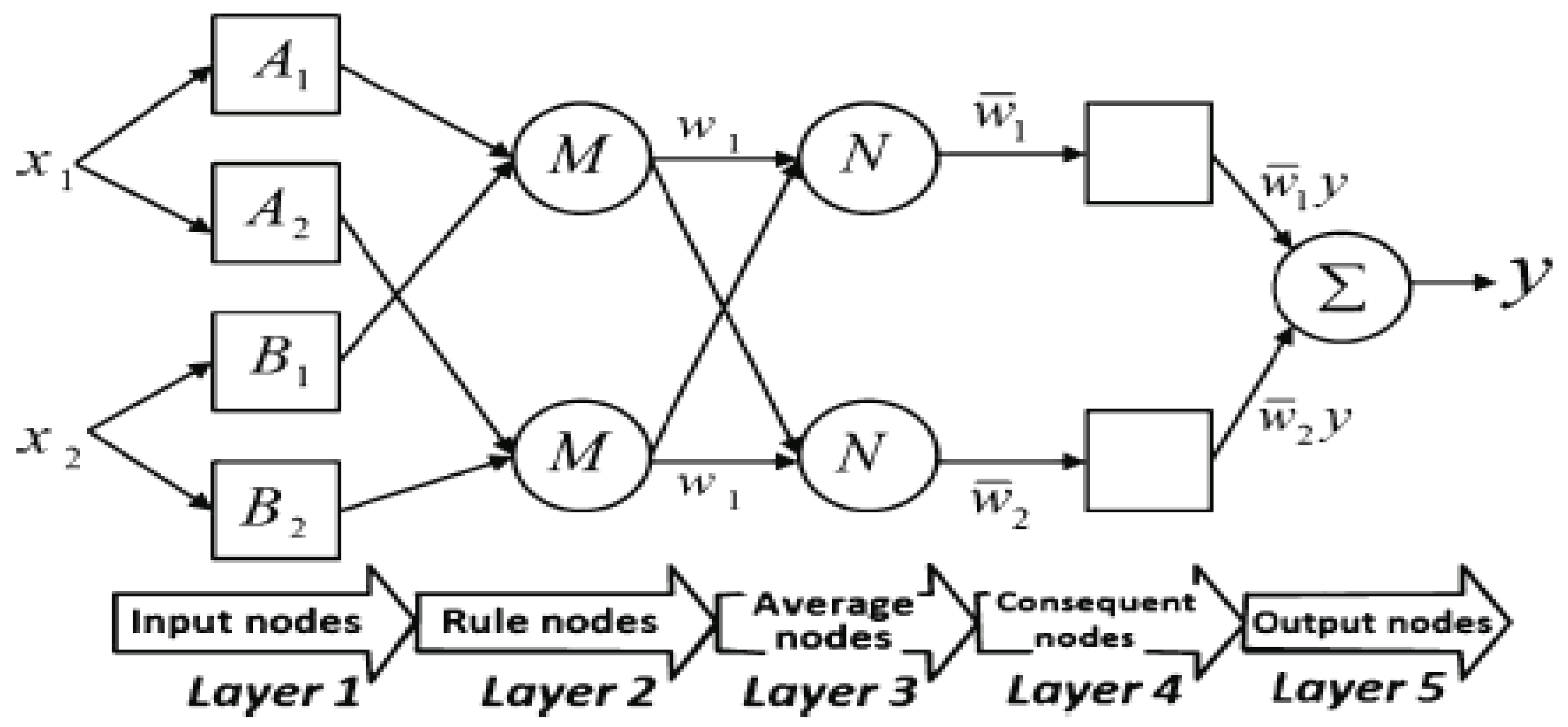
2.1. Adaptive Neuro-Fuzzy Inference System

ANFIS is an advanced feed forward network containing several layers, and analyzes each incoming signal node with a specific function [27]. Square node and circle node codes are used to illustrate different qualities of adaptive learning. To obtain the required input and output attributes, adaptive learning parameters are developed on the basis of gradual learning rules. The ANFIS membership functions are based on the rules and membership functions of the data [27]. Essentially, the fuzzy inference system explained here contains two inputs (x₁ and x₂) and only one output (y). It is assumed that the rule base contains two fuzzy IF-THEN rules of a first-order Sugeno fuzzy [28].

Rule 1: If x₁ is A₁ and x₂ is B₁, then y₁ = f₁ = p₁x₁ + q₁x₂ + r₁

(1)

Rule 2: If x₁ is A₁ and x₂ is B₁, then y₂ = f₂ = p₂x₁ + q₂x₂ + r₂

(2)

where A_i and B_i are the fuzzy sets and p_i, q_i, and r_i that it is the design parameters to be identified during calibrations and validation processes.

The architecture of ANFIS is shown in Figure 1, in which circles nodes and squares describe adaptive nodes. The following paragraph provides a brief introduction to the ANFIS model.

Input nodes (layer 1): Each node i of this layer is a square node with a node function. In fuzzy system, for input values x₁ and x₂, the inferred output y is estimated by using Equation (3) [29]:

$$\begin{gathered} O_{1,i}={\mu }_{A_i}\left(x_1\right),i=1,2 \\ {O}_{1,i}={\mu }_{B_{i-2}}\left(x_1\right),i=3,4 \end{gathered}$$

(3)

where x₁ and x₂ are the inputs to node $i$, $A_i$ and $B_i$ are the linguistic labels, and $\mu A_i$ and $\mu B_{Bi-2}$ are the membership function for the $A_i$ and $B_i$ linguistic labels, respectively.

Rule nodes (layer 2): Every node in this layer is a circle node labeled as M (Figure 1). The outputs of this layer, which are called firing strengths ($O_{2,i}$), are the products of the corresponding degrees obtained from layer 1 (input layer).

$$O_{2,i}=w_i= {\mu }_{A_i}\left(x_1\right)* {\mu }_{B_i}\left(x_1\right),i=1,2$$

(4)

Average nodes (layer 3): Every node in this layer is a circle node labeled as N (Figure 1). The third layer contains fixed nodes that calculate the ratio of the firing strengths of the rules:

$$O_{3,i}={\mathsf{ẃ}}_i=\frac{W_i}{W_1+W_2} ,i=1,2$$

(5)

Consequent nodes (layer 4): The nodes in this layer are adaptive, and the output of each node is simply the product of the normalized firing strength and a first order polynomial. Thus, the output and the function are defined by the following equation:

$$O_{4,i}={\mathsf{ẃ}}_i{y}_i={\mathsf{ẃ}}_i\left(p_{i}x+q_{i}y+r_i\right),i=1,2$$

(6)

The parameters, $p_i$, $q_i$, and $r_i$ in this layer are the coefficients of this linear combination and can be referred to as the consequent parameters.

Output nodes (layer 5): The single node computes the overall output by summing up all of the incoming signals.

$$O_{5,i}={\displaystyle \sum }_{i=1}^2{w}_i{y}_i=\frac{{{\displaystyle \sum }}_{i=1}^2{w}_{i}y}{w_1+w_2}$$

(7)

The details and mathematical background for these algorithms can be found in [27].

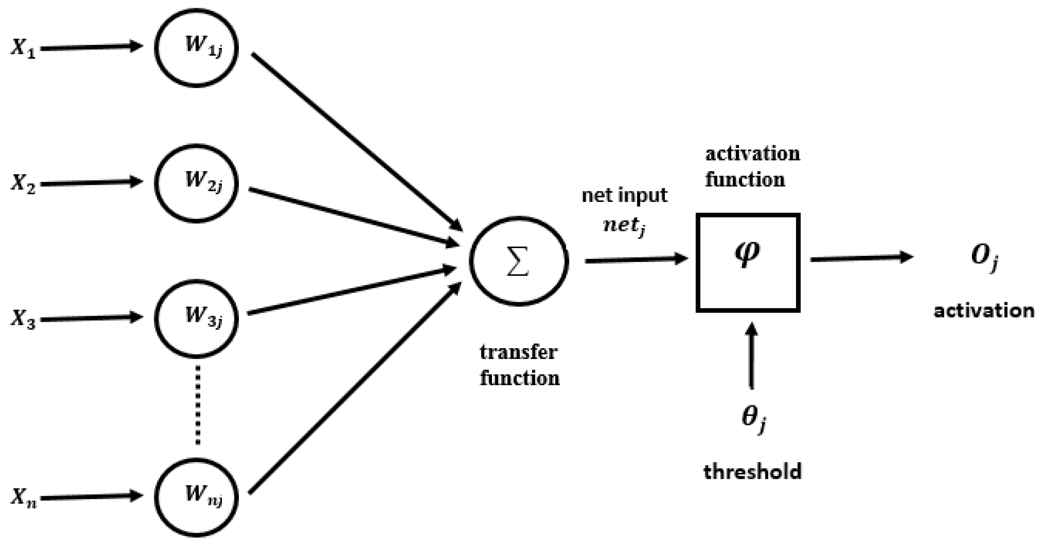
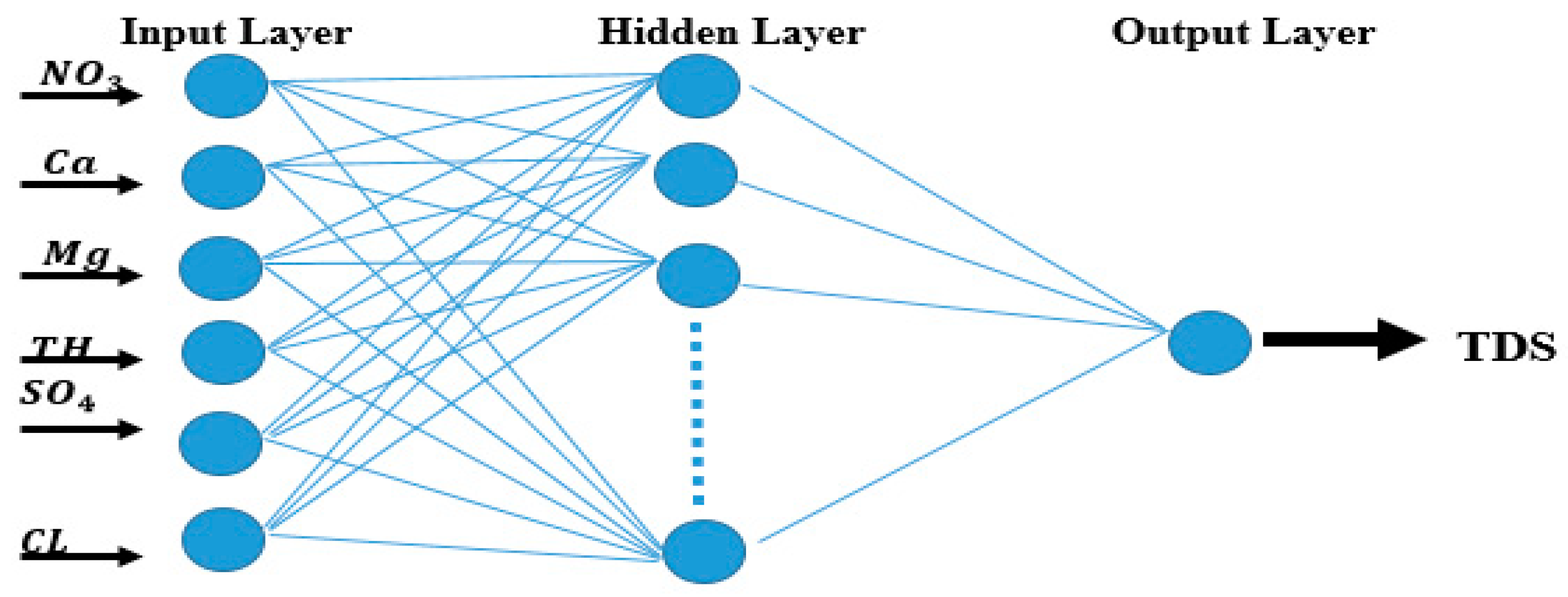
2.2. Artificial Neural Network

An artificial neuron is the primary building step for all ANN. It has the same design and characteristics in natural neurons in biological neural networks [1]. Figure 2 shows the architecture of the artificial neuron with inputs variable, weights, transfer functions, activation functions, threshold and output.

The artificial neuron is fed by numbers of inputs. Depending on the value of the weight, the effect of the transfer function and output, the effect of the all inputs on the neuron will be different. from the calculation of the transfer function and output. Generally, greater weight values result in higher power and affect the associated inputs. Since all the inputs are multiplied by their corresponding weight, the weights will influence the neurons output. The transfer function as a summation of the weighted inputs is used to produce the net input to the neuron [30], as provided in Equation (8).

$$netj={\displaystyle \sum }_{i=1}^n{w}_{ij}{x}_i+b$$

(8)

where j is the actual neuron number, $x_i$ is an input value, $i$ from 1 to $n$, $w_{ij}$ is a weight value and $b$ is equal to the negative threshold value of a neuron and called the bias of the neuron.

In addition to

$$x_j=\phi \left(u_j-{\theta }_j\right)$$

(9)

where $x_{j }\mathrm{output}\mathrm{signal}, {\theta }_j$ is the bias term of the $j$ neuron [30,31]. The logistic sigmoid function, Bilgili and Yasar 2007 is used for this purpose [32], expressed as given in Equation (10).

$${\phi }_x=\frac{1}{1+e^{-x}}$$

(10)

In this study, a feed forward-back propagation with MLP neural network was used. The network was trained using Levenberg–Marquardt. The structure of ANN model with two layers used in this study is shown in Figure 3. This training algorithm helps in distributing the error in order to arrive at a best fit or minimum error [22], and it is the most commonly used class of ANNs [15]. The transfer function between layer one and layer two was log sigmoid. The types of the transfer function in neural networks are log-sigmoid, tan-sigmoid, and pure-linear function. The main reason why we use log-sigmoid function is because it exists between (0 to 1). Therefore, it is especially used for models where we have to predict the probability as an output. Since probability of anything exists only between the range of 0 and 1. The optimal number of neurons in the hidden layer was selected based on the trial and error method by changing the number of neurons in the hidden layer from 1 to 5.

2.3. Multiple Linear Regression

In the multiple linear regression (MLR) method, a dependent variable is assumed to be a linear function of one variable. A simple linear regression model and the relationship between observed and estimated value of dependent variable can be specified as [33]:

$$Y =a+bX$$

(11)

$$Y_i =a+bX+ {\epsilon }_i$$

(12)

where $Y$ is the measured value, $Y_i$ is the calculated value, $a$ is the constant, $b$ is slope, ${\epsilon }_i$ is the error associated with estimate of $Y_i$, and the value of $X$ = $x_i$ is the given value of the independent variable. The constants $a$ and $b$ are estimated by ordinary least squares. If ${\epsilon }_i=0$, the calculated value ($Y$) is equal to measured value ($Y_i$).

MLR is very similar to simple linear regression but the difference in MLR is that the dependent variable is a function for more than one independent variable. MLR model can be specified as given in Equation (13):

$$Y_i=a+ b_1{X}_1+b_2{X}_2\dots +b_n{X}_n+ {\epsilon }_i$$

(13)

where $Y_i$, $a$ and ${\epsilon }_i$ have described above, $b_1$, $b_2$ …, $b_n$ are the partial regression (slope) parameter for $X_1$, $X_2$ …, $X_n$. The main purpose of using MLR is to find the linear relationship between dependent and independent variables and to obtain a linear model using regression coefficients as well as to calculate the dependent variable. For the best-calculated value of the dependent variable, ${\epsilon }_i$ can be specified as given in Equation (14):

$${\displaystyle \sum }_{i=1}^n{\left({\epsilon }_i\right)}^2={\displaystyle \sum }_{i=1}^n{\left(Y_i-a+ b_i{X}_1+ b_2{X}_2+ \dots + b_n{X}_n\right)}^2$$

(14)

3. Study Area and Data

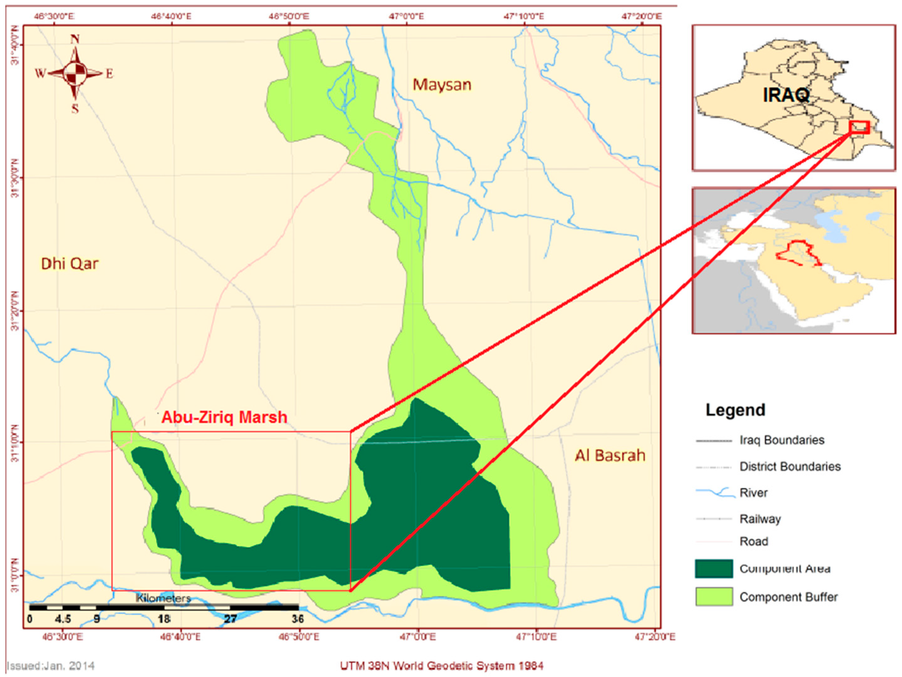
3.1. Abu-Ziriq Marsh Description

In this study, Abu Ziriq marsh was selected as a case study. To the best of the author’s knowledge, no previous studies addressed the water quality modeling in this area. Abu-Ziriq marsh, which covers 120 km², it is about 3% of all marshes area, lies at the tail end of Al Gharraf River southerly of Al Islah district at a location of latitude 31°09′54.9″ N, longitude 46°36′33″ E. The main source of water supply to the marsh is through Shatt Abo-Lihia and the channel of this river runs through the marsh until it dissipates at the tail end into the central marshes. The two main towns around the marsh are Al-Islah in the North and Al-Fuhod in the south of Thi Qar governorate (Figure 4). Scattered villages of fishermen are located all along the embankments that surround the marsh. Highlighting the vitality role of Abu-Ziriq marsh in sustaining the daily life of the local residents. The success of the models used in this study gives the possibility to be used in the rest of the marshes which means reducing the cost and time of water quality monitoring.

3.2. Water Sampling Procedure

The dataset utilized in this paper was collected and observed consistently, every month, at Abu-Ziriq marsh by the Ministry of the Environment, Department of Protection and Improvement Environment in the south of Iraq. The final dataset of water quality consisted of 84 monthly records collected between years 2009 to 2018 (

Table 1. Monthly records of water quality parameters per year.

Year	2009	2010	2013	2014	2015	2016	2017	2018
Sample of data	11	9	12	12	12	8	12	8

). Each record consists of eight parameters, namely: ${\mathrm{NO}}_3$, ${\mathrm{Ca}}^{+2}$, ${\mathrm{Mg}}^{+2}$, $\mathrm{T}.\mathrm{H}$, ${\mathrm{SO}}_4$, ${\mathrm{Cl}}^{-1}$, $\mathrm{EC}$ and $\mathrm{TDS}$. These variables are used to develop the ANFIS, ANN and MLR models.

Table 2. Summary of statistical parameters of input and output variables (n = 84).

Variable	Unit	Range	Min	Max	Mean	SD	CV%
${\mathrm{NO}}_3$	ppm	3.50	0.30	3.80	1.45	0.52	0.27
${\mathrm{Ca}}^{+2}$	ppm	736	64	800	160.84	94.52	8935
${\mathrm{Mg}}^{+2}$	ppm	310	20	330	97.58	65.49	4290.04
T.H	ppm	1840	320	2160	783.20	394.79	155,866.64
${\mathrm{SO}}_4$	ppm	1201	99	1300	430.25	278.25	77,427.58
Cl−1	ppm	1472	150	1622	481.28	312.45	97,626.15
EC	µS/cm	6620	1200	7820	3072.13	1676.71	2,811,366
TDS	ppm	4006	614	4620	1781.19	960.22	922,029.31

SD standard deviation, CV coefficient of variation, Ca—calcium, Cl—chlorine, EC—electrical conductivity, NO₃—Nitrate, Mg—magnesium, SO₄—sulfate, TDS—total dissolved solids.

lists the statistical parameters of water quality in the marsh. The parameters for $\mathrm{EC}$ and $\mathrm{TDS}$ were chosen based on strong Pearson correlation at significance level of 0.01. While the weak cross-correlation parameters are neglected (

Table 3. Correlation matrix among water quality parameters.

Parameters	NO3	Ca+2	Mg+2	T.H	SO4	Cl−1	EC	TDS
NO3	1
Ca+2	0.225	1
Mg+2	0.139	0.487	1
T.H	0.149	0.582	0.943	1
SO4	0.103	0.559	0.878	0.894	1
Cl−1	0.293	0.685	0.828	0.894	0.855	1
EC	0.193	0.640	0.887	0.922	0.930	0.955	1
TDS	0.220	0.636	0.875	0.920	0.917	0.966	0.988	1

Ca—calcium, Cl—chlorine, EC—electrical conductivity, NO₃—Nitrate, Mg—magnesium, SO₄—sulfate, TDS—total dissolved solids. All the values were significant at alpha < 0.01.

). The advantages of adopting these special variables are greatly improving network performance. In this paper, the total Abu-Ziriq water quality dataset (84 samples) were randomly divided into two groups: calibration and validation. The calibration and validation datasets comprised of 63 (75%) and 21 (25%) samples, respectively.

4. Performance Measures

Several criteria have been used in the literature for the assessment of model performance such as Mean Absolute Error, Normalized Root Mean Square Error, Threshold Statistics, Root Mean Squared Error, Correlation Coefficient and Nash–Sutcliffe Coefficient of Efficiency [24,34,35]. In this study, the following three criteria were employed as they are widely used in evaluating water quality models [35].

• The Root Mean Squared Error (RMSE): RMSE is an error index type parameter commonly used in hydrological modeling:

  $$\mathrm{RMSE}=\sqrt{\frac{{{\displaystyle \sum }}_{i=1}^n{\left(M_i-P_i\right)}^2}{N}}$$

  (15)

  where $M_i$ is measured value, $N$ is number of data set and $P_i$ is predicted value. For RMSE, a value of zero is the optimum.
• Correlation Coefficient (CC): CC is a standard regression type parameter and defined as a measure of the strength of the linear relationship between the measured and predicted or estimated datasets:

  $$\mathrm{CC}=\frac{{{\displaystyle \sum }}_{i=1}^N\left(\left(M_i-\mathsf{\mu })(P_i-\mathsf{Ṕ}\right)\right)}{\sqrt{{{\displaystyle \sum }}_{i=1}^N({\left(M_i-\mathsf{\mu }\right)}^2{\left(P_i-\mathsf{Ṕ}\right)}^2)}}$$

  (16)

  where N is the number of input samples; $M_i$ and $P_i$ are the measured and network output value from the elements, respectively. µ and $\mathsf{Ṕ}$ and are their average, respectively.
• The Nash–Sutcliffe Coefficient of Efficiency (NSE): NSE is a dimensionless type parameter widely used as a metric of model efficiency [36]:

  $$\mathrm{NSE}=\frac{{{\displaystyle \sum }}_{i=1}^N{\left(M_i-\mathsf{\mu }\right)}^2-{{\displaystyle \sum }}_{i=1}^N{\left(P_i-M_i\right)}^2}{{{\displaystyle \sum }}_{i=1}^N{\left(M_i-\mathsf{\mu }\right)}^2}$$

  (17)

NSE ranges from −1 to +1, with better models giving NSE values as close to 1 as possible.

5. Results and Discussion

5.1. Model Structure

Given its importance in terms of the Abu-Ziriq marsh water quality, electrical conductivity (EC) and total dissolved solids (TDS) were chosen as the water quality parameters of interest. The chemical parameters, namely: NO₃, Ca⁺², Mg⁺², T.H, SO₄, Cl⁻¹, EC and TDS were assessed (Table 2), for Abu-Ziriq marsh water samples collected on the monthly basis by the Ministry of the Environment, Department of Protection and Improvement Environment in the south of Iraq over the period of January 2009 to August 2018 at the Abu-Ziriq station. An important thing to do in developing a prediction model is to choose the correct input parameters. The parameters for EC and TDS were chosen based on strong Pearson correlation at significance level of 0.01. While the weak cross-correlation parameters are neglected (Table 3). Cross-correlation is used for measuring the similarity of two series as a function of the displacement of one relative to the other [37]. Table 3 tabulates the correlation matrix between the water quality parameters. Based on Pearson correlation coefficient with p < 0.01, the parameters used as inputs in modeling EC were the concentrations of Ca⁺², Mg⁺², T.H, SO₄, and Cl⁻¹. While the parameters used as inputs in modeling TDS were the concentrations of NO₃, Ca⁺², Mg⁺², T.H, SO₄ and Cl⁻¹ (Table 3). Apparently, there was no remarkable difference between the model structure of EC and TDS. The only difference was the component of NO₃. This might be attributed to the weak Pearson cross-correlation (0.193) at significance level >0.05, therefore, it is neglected.

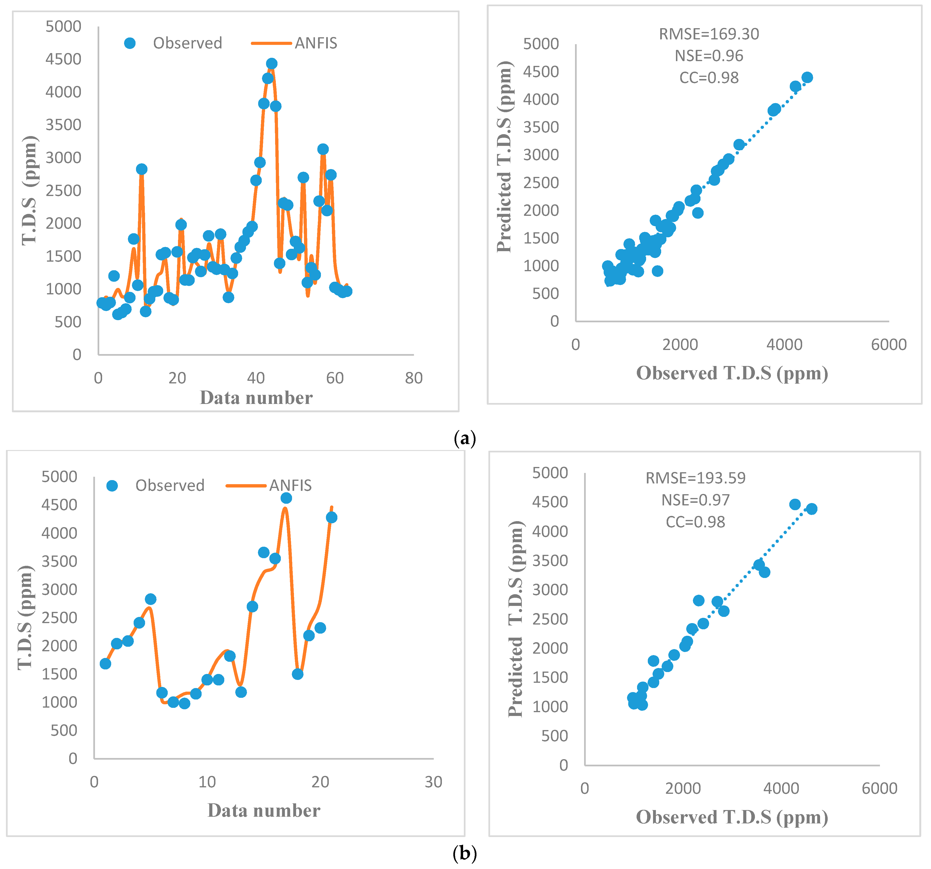
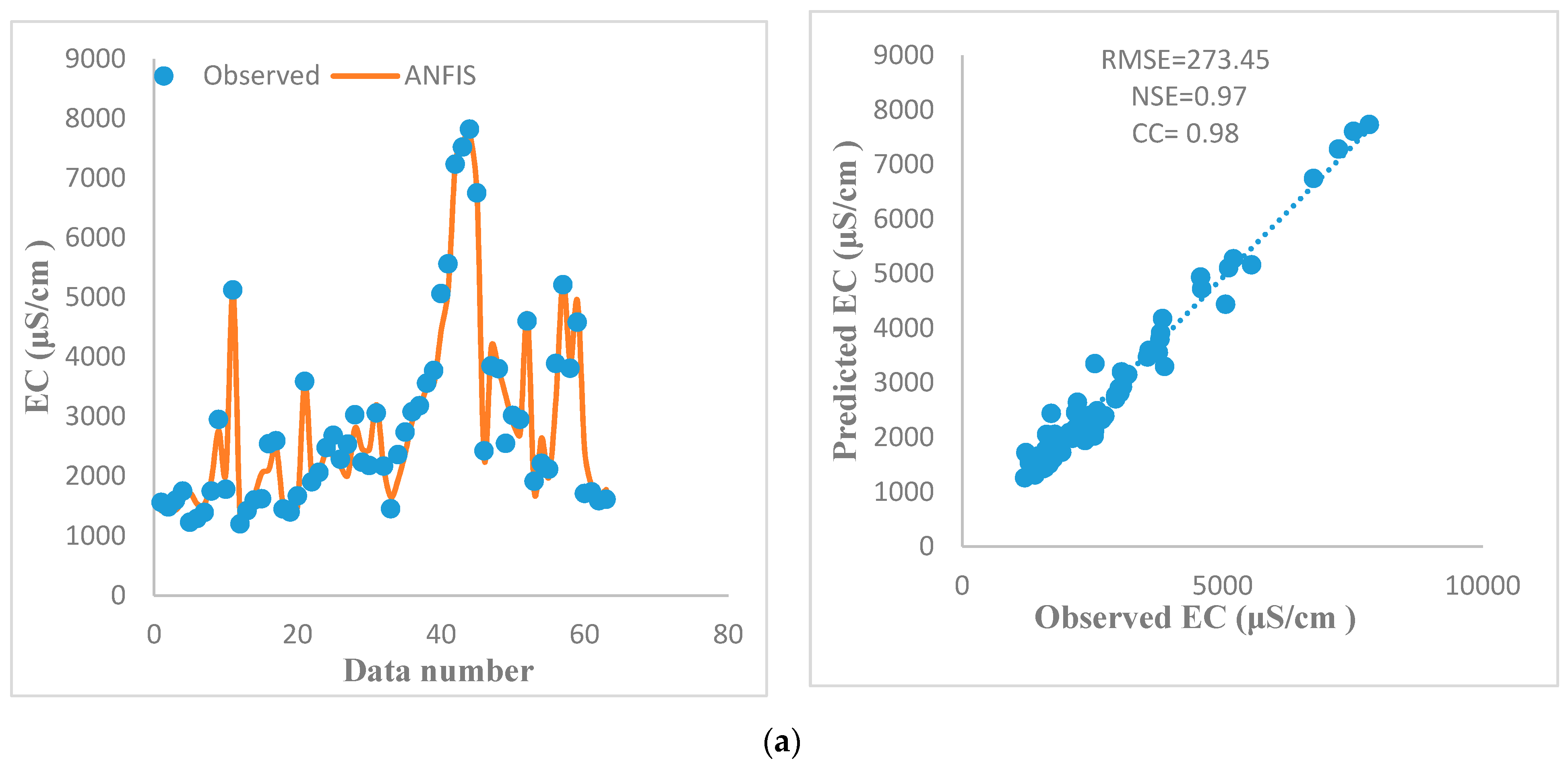
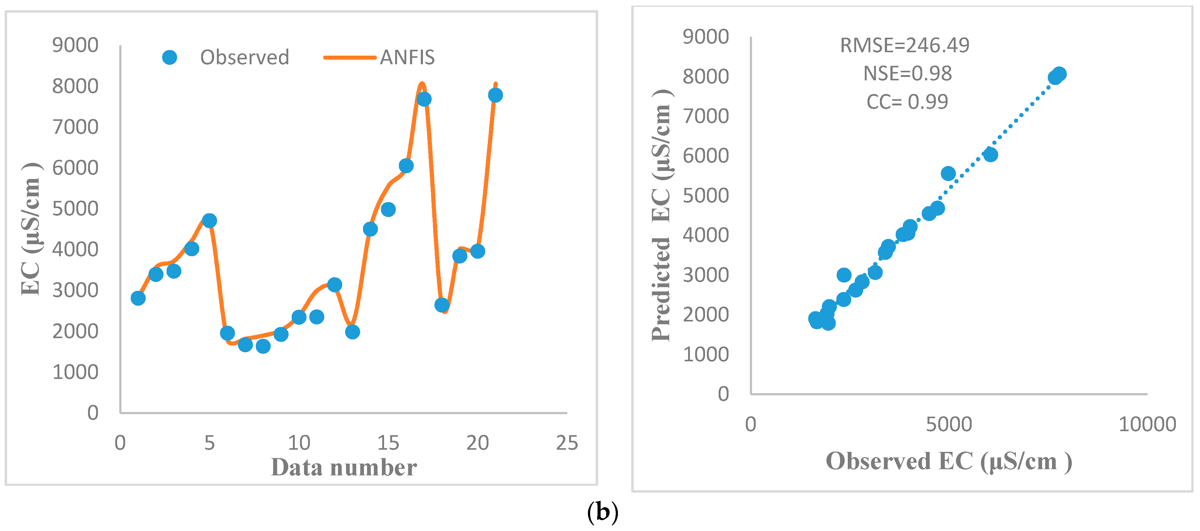
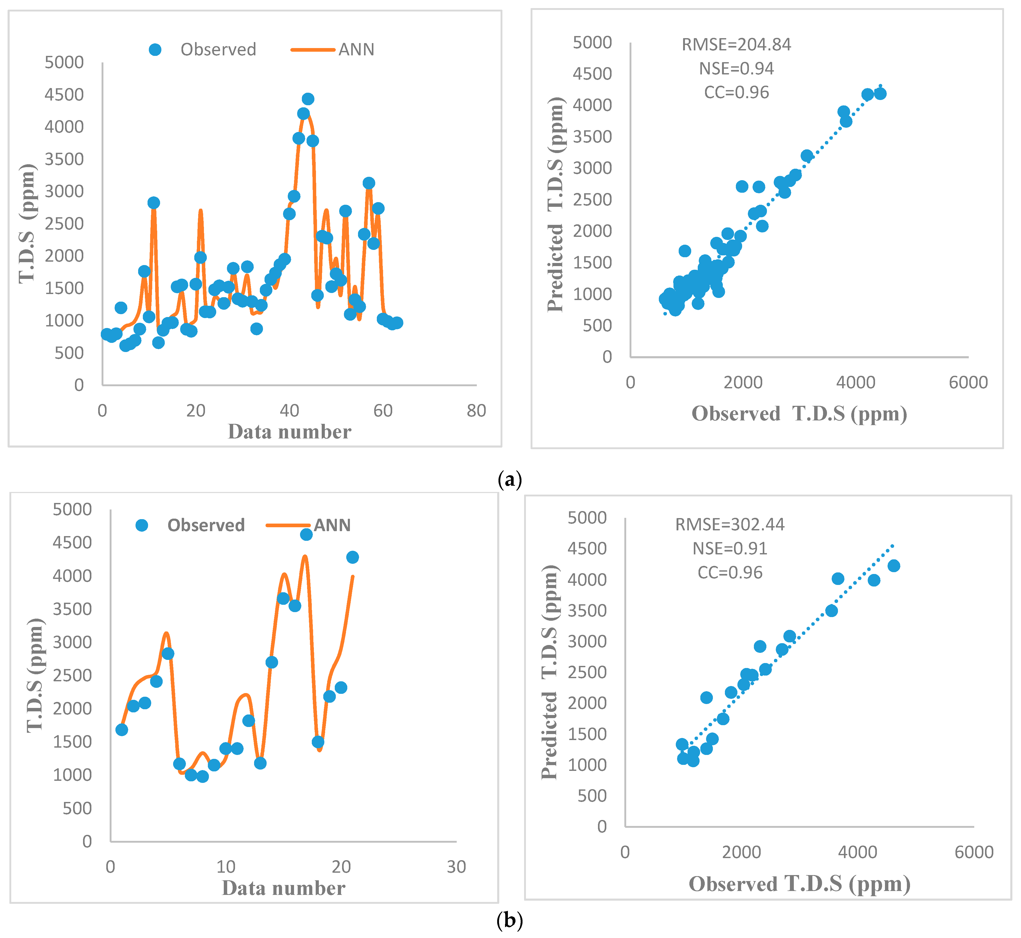
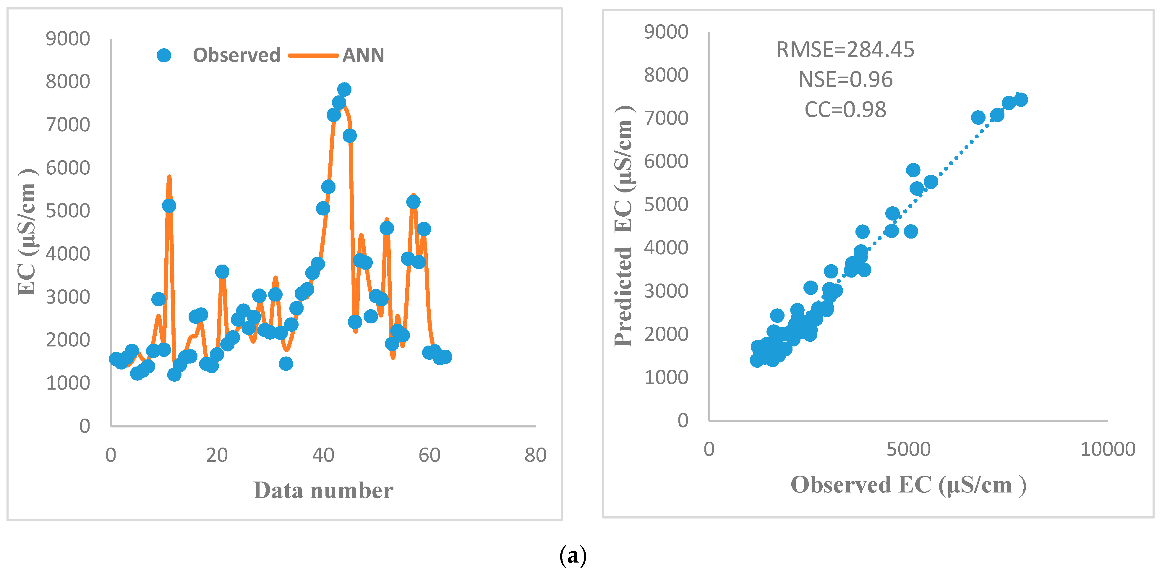
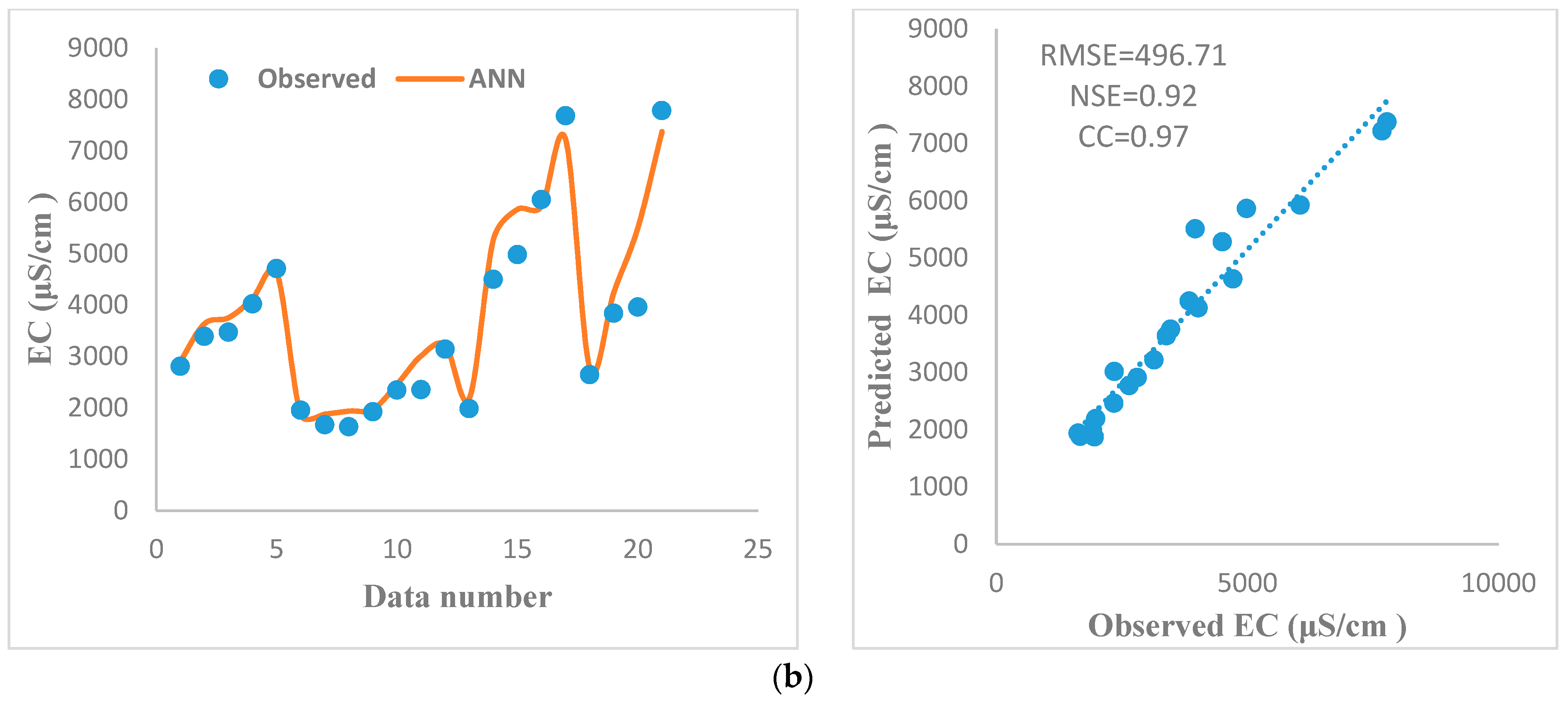
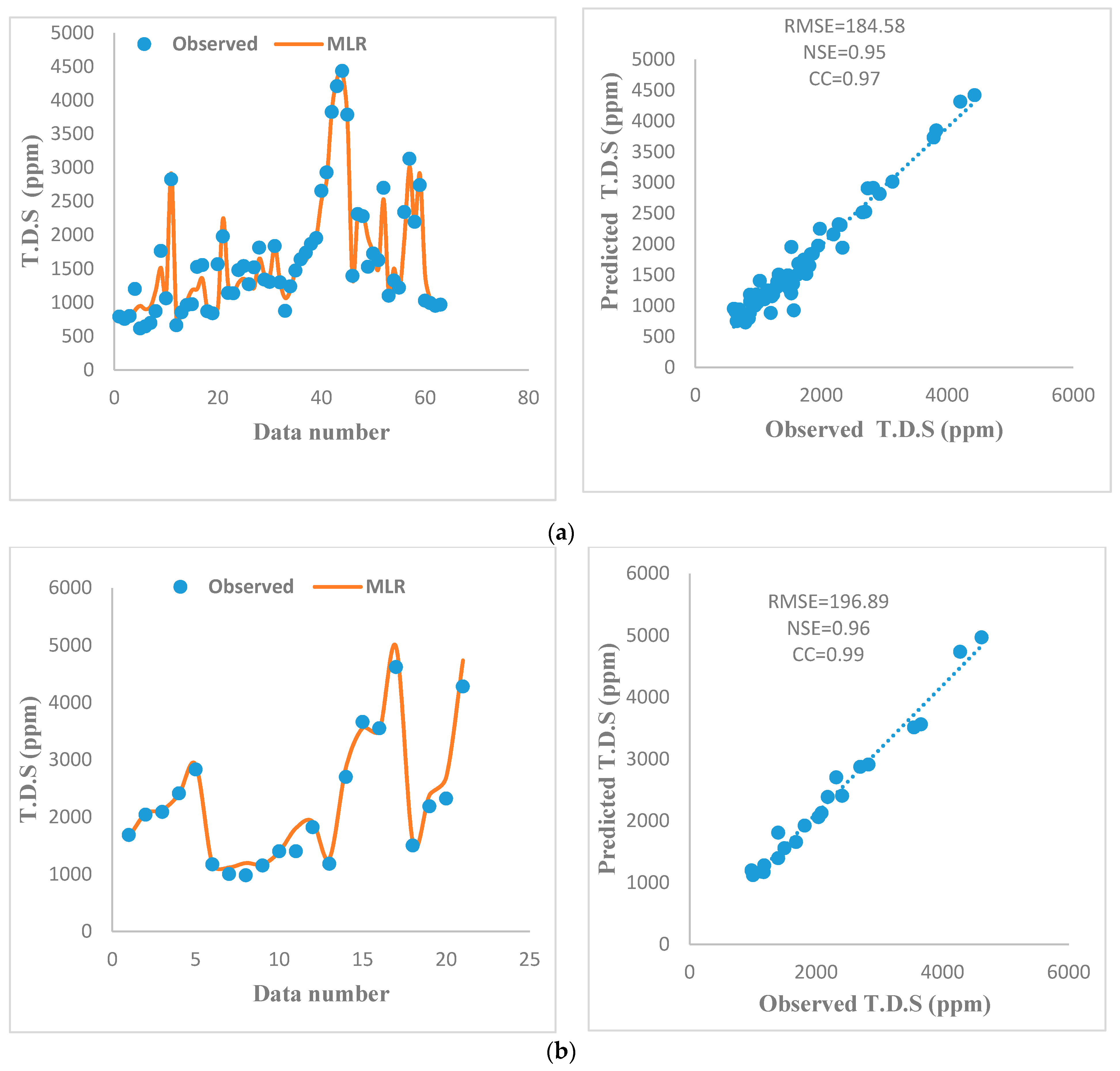
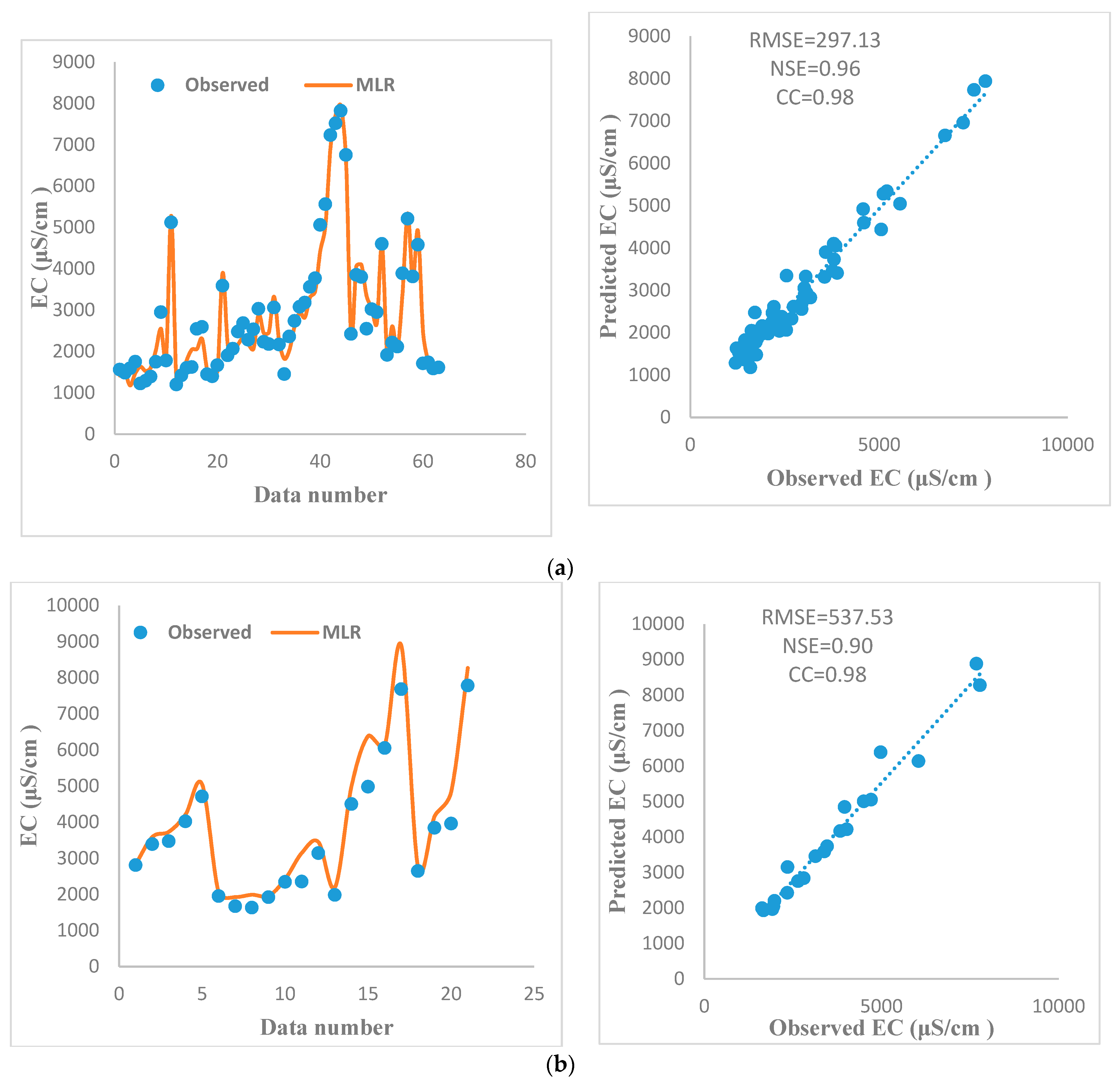
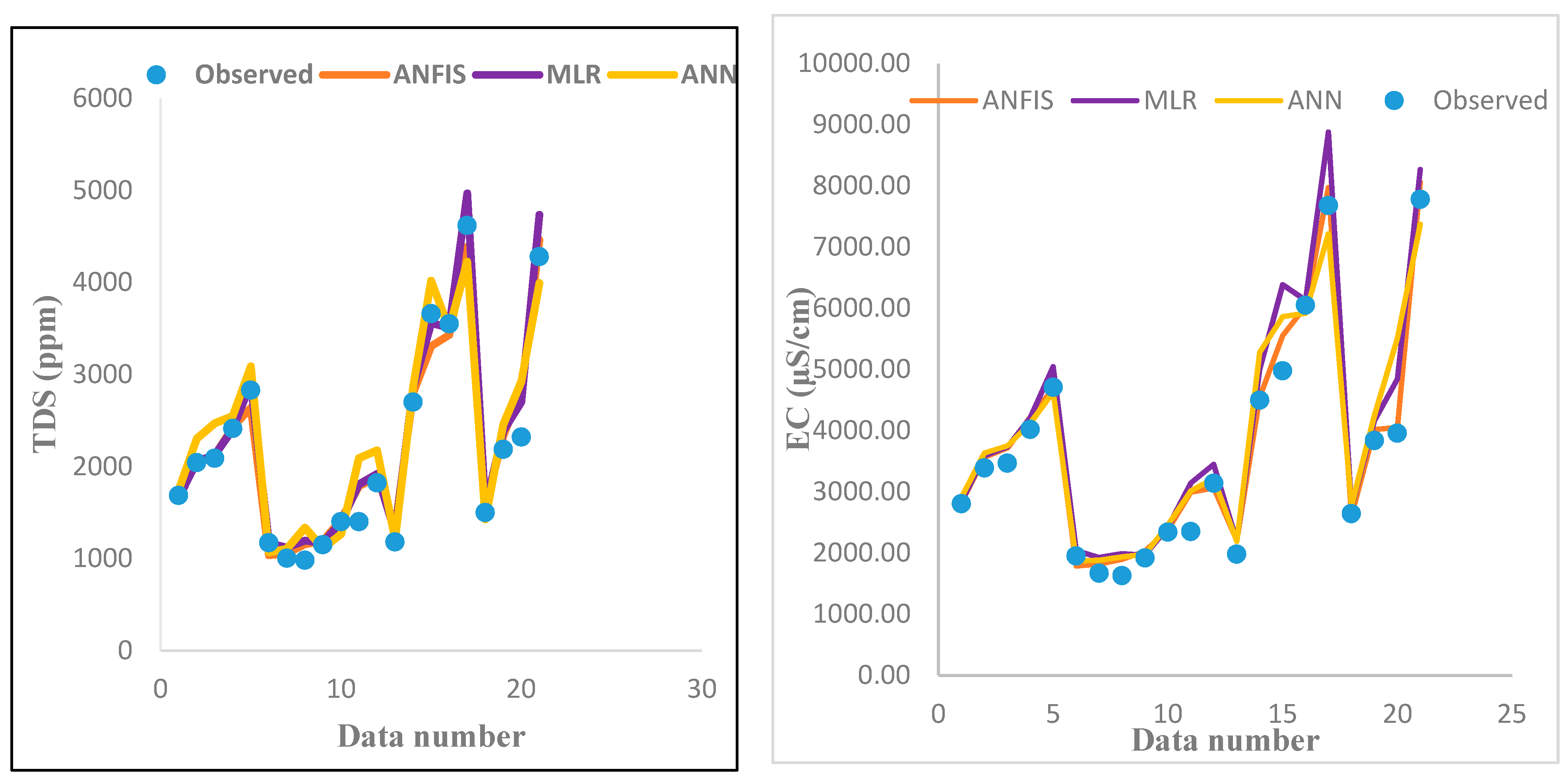
5.2. Models Performance

In this study, nitrate (NO₃), calcium (Ca⁺²), magnesium (Mg⁺²), total hardness (T.H), sulfate (SO₄), chloride (Cl⁻¹), electrical conductivity (EC) and total dissolved solids (TDS) in Abu-Ziriq, south of Iraq, were used to develop artificial intelligence techniques. The TDS and EC models were created by utilizing ANFIS, ANNs and MLR.

In ANFIS modeling, there are two types; Sugeno and Mamdani, where the first one can be further subdivided into two types: hybrid and back propagation. Membership function types for input and output parameters were considered as Sugeno fuzzy Gaussian (gaussmf), backpropagation algorithm and linear MFs, respectively. This method creates a FIS for which membership-function parameters are adjusted using either aback propagation algorithm alone or a combination of aback propagation algorithm and a least-squares method [38]. The number of membership functions for each input of ANFIS for TDS and EC were set to (2,2,2,1,2,3) and (2,3,1,3,2), respectively. The performance of the ANFIS model for the calibration and validation datasets are given in

Table 4. Comparison of ANFIS, ANN and multiple linear regression (MLR) models performance.

Estimated	Model	Calibration			Validation
		RMSE	CC	NSE	RMSE	CC	NSE
TDS	MLR	184.58 (ppm)	0.97	0.95	196.89 (ppm)	0.99	0.96
	ANN	204.84 (ppm)	0.96	0.94	302.14 (ppm)	0.96	0.91
	ANFIS	169.30 (ppm)	0.98	0.96	193.59 (ppm)	0.98	0.97
EC	MLR	297.13 (μS/cm)	0.98	0.96	537.53 (μS/cm)	0.98	0.90
	ANN	284.45 (μS/cm)	0.98	0.96	496.71 (μS/cm)	0.97	0.92
	ANFIS	273.45 (μS/cm)	0.98	0.97	246.49 (μS/cm)	0.99	0.98

. Figure 5 shows the observed versus predicted TDS from ANFIS model during the calibration and validation periods. As it can be seen in the figure, there was a satisfactory matching between both data sets. Moreover, values of RMSE, CC, and NSE were 169, 30, 0.98 and 0.96, respectively for the calibration and 193.59, 0.98 and 0.97, respectively for the validation of datasets (Table 4). While, Figure 6 shows the observed versus predicted EC from ANFIS model during the calibration and validation periods. As it can be noticed from the figure, there was a satisfactory matching between both data sets. This was clarified through values of RMSE, CC, and NSE, which were 273.45, 0.98 and 0.97, respectively for calibration data set and 246.49, 0.99 and 0.98, respectively for validation. In their study, Kisi and Ay reported superior performance of ANFIS in comparison to MLR in modeling monthly mean dissolved oxygen concentration in Broad River, USA [26].

In ANN modeling, feed forward-backpropagation algorithm, Levenberg–Marquardt training algorithm (TrainLM), were constructed to estimate TDS and EC values. The transfer function between layer one and layer two was (LOGSIG). The optimal number of neurons in the hidden layer was selected using the trial and error method, by experimenting with changing the number of neurons in the hidden layer from 1 to 5. The optimal number of neurons in the hidden layers providing the optimal structure was determined as 3 for TDS and 2 for EC. Therefore, ANN (6, 3, 1) was selected as the optimum ANN model for TDS and ANN (5, 2, 1) for EC. The performance of the ANN model for the calibration and validation of datasets are given in Table 4. Figure 7 shows the observed versus predicted TDS from ANN model during the calibration and validation periods. As it can be shown from the figure, there was an adequate consistency between both data sets. In addition, values of RMSE, CC, and NSE were 204.84, 0.96, and 0.94, respectively for calibration data set and 302.44, 0.96 and 0.91, respectively for validation. On the other side, Figure 8 shows the observed versus predicted EC from ANN model during the calibration and validation periods. As it can be seen from the figure, both data sets were in a good consistency. Moreover, values of RMSE, CC, and NSE were 284.45, 0.98 and 0.96, respectively for calibration and 496.71, 0.92 and 0.97, respectively for the validation data set. Barzegar et al. applied ANFIS and ANN model to estimate water electrical conductivity at Aji-Chay River, northwest of Iran. ANN model could not achieve a high efficiency to estimate water electrical conductivity [34].

The performance of the MLR model and equation for the calibration and validation are given in Table 4;

Table 5. MLR model Eq.

$\mathrm{EC}=466.309-0.607\mathrm{Ca}+4.973\mathrm{Mg}-0.3628\mathrm{T}.\mathrm{H}+1.523{\mathrm{So}}_4+\mathrm{4.0.398}\mathrm{Cl}.$

$\mathrm{TDS}=\mathrm{3.25.866}-35.531{\mathrm{No}}_3-0.377\mathrm{Ca}+2.239\mathrm{Mg}-0.003\mathrm{T}.\mathrm{H}+0.643{\mathrm{So}}_4+2.299\mathrm{Cl}$

. Figure 9 shows the comparative plots of the results obtained From MLR model for TDS during the calibration and validation periods. RMSE, CC, and NSE values set were 184.58, 0.97 and 0.95 for the calibration dataset, respectively. While these values for the validation dataset were 196.89 ppm, 0.99 and 0.96, respectively.

In addition, MLR model was used to estimate EC, the performance model for the calibration and validation were plotted as shown in Figure 10. It can be noticed that both data sets were consistent. In other words, MLR model’s performance was satisfactory in modeling EC. However, RMSE, CC, and NSE values set were 297.13 μS/cm, 0.98 and 0.96, respectively for the calibration, while these values for the validation were 537.53 μS/cm, 0.98 and 0.90, respectively. Nemati et al. [15] used ANFIS, ANN and MLR models to estimate water quality parameter in the Tai Po River, Hong Kong. They found that MLR model did not have the high accuracy to estimate DO. Chen and Liu applied ANN, ANFIS and MLR models to estimate DO concentration in the Feitsui Reservoir of Northern Taiwan. The result show that MLR model was not be able to estimate DO [11].

From aforementioned, it can be concluded that the ANFIS model outperformed the ANN and MLR models on the three performance criteria: RMSE, CC and NSE during the calibration and validation periods Table 4. Figure 11 shows the time series of the developed models for validation dataset. It can be seen from Figure 11 that the all models give similar estimates for the TDS and EC values. This might be attributed to its sophisticated structure and the capability of eliminating the noisy data [39], ANFIS model (Sugeno) makes use of “IF–THEN” rules to produce an output for each rule [40], This allows to learn from the data [41]. The neuro-fuzzy systems have an advantage of both ANFIS and ANNs, that is benefiting from the training ability of the ANN and the fuzzy IF–THEN rule generation and parameter optimization [42]. Our findings are in parallel with previous studies [10,24,26,43,44], where they proved the superior performance of ANFIS in modeling hydrological and water quality parameters.

5.3. Sensitivity Analysis

Sensitivity analysis was used to investigate the effects of the input variables on the model outputs [45]. To this end, a percentage change in EC and TDS were determined by considering 10%, 20%, 30%, 40%, and 50% increase/decrease changes in their respective input parameters using the optimal model. Results of sensitivity analysis were tabulated as shown in

Table 6. Sensitivity analysis of input parameters on EC and TDS in Abu-Ziriq Marsh using ANFIS model.

Input parameters	−10%	−20%	−30%	−40%	−50%	+10%	+20%	+30%	+40%	+50%
EC	7.01	16.55	26.18	35.65	45.27	−11.5	−20.65	−29.55	−37.93	−45.64
TDS	3.28	13.91	25.53	37.1	48.8	−17.83	−27.53	−33.83	−41.93	−47.65

. ANFIS. Results of EC from ANFIS showed an increase by 7.01%, 16.55%, 26.18%, 35.65% and 45.27%, from the 10%, 20%, 30%, 40%, 50% increase change, respectively. While sensitivity were −11.5%, −20.65%, −29.65%, −37.93% and −45.65%, respectively from the decrease change.

On the other hand, the effect of a decrease in input by 10%, 20%, 30%, 40%, and 50% causes an increase in TDS by 3.28%, 13.91%, 25.53%, 37.1% and 48.8%. While the decrease change in the input parameters showed decreased by −17.83%, −27.53%, −33.83%, −41.93% and −47.65% when ANFIS input was increased by 10%, 20%, 30%, 40% and 50%, respectively.

An increase/decrease in the inputs parameters causes similar increase/decrease in the EC and TDS. This could be interpreted by the physical association among the data. Concentrations of ions exist in water samples is coherent with the amount of discharges received to the marsh. In other words, the lower the discharge, the higher ions concentrations.

Therefore, in order to maintain a good water quality index in the marsh, certain water discharges should be sustained. This would be addressed in future study.

6. Conclusions

This study evaluated three different types of artificial intelligence ANFIS, ANN, and MLR neural networks to calculate and predict TDS and EC at Abu-Ziriq marsh in the south of Iraq. Three assessment criteria were used for the evaluation such as CC, RMSE, and NSE. It was found that the ANFIS outperformed the other evaluated methods. In other words, ANFIS model led to the best fit with the observed data. This could be attributed to the ANFIS structure. The ANFIS integrates the advantage of the simplifying function of fuzzy reasoning and the self-learning ability of neural networks and thus gives a strong capability of eliminating noise [46]. ANFIS is recommended to be used as a predictive model for water quality parameters (TDS and EC) in the Iraqi marshes. The utilization of applied methods in this study can be considered in other marshes and rivers in order to investigate the generalization of the methods. Furthermore, the tools applied in current paper could provide a basis for managers, engineers and policymakers for impressive design, management and decision making over different marshes or rivers and basins of Iraq.

References

1. Singh, K.P.; Malik, A.; Mohan, D.; Sinha, S. Multivariate statistical techniques for the evaluation of spatial and temporal variations in water quality of Gomti River (India)—A case study. Water Res. 2004, 38, 3980–3992. [Google Scholar] [CrossRef] [PubMed]
2. Sattari, M.T.; Joudi, A.R.; Kusiak, A. Estimation of water quality parameters with data-driven model. J. Am. Water Works Assoc. 2016, 108, E232–E239. [Google Scholar] [CrossRef]
3. Basant, N.; Gupta, S.; Malik, A.; Singh, K.P. Linear and nonlinear modeling for simultaneous prediction of dissolved oxygen and biochemical oxygen demand of the surface water—A case study. Chemom. Intell. Lab. Syst. 2010, 104, 172–180. [Google Scholar] [CrossRef]
4. Dogan, E.; Sengorur, B.; Koklu, R. Modeling biological oxygen demand of the Melen River in Turkey using an artificial neural network technique. J. Environ. Manag. 2009, 90, 1229–1235. [Google Scholar] [CrossRef]
5. Firat, M.; Güngör, M. Monthly total sediment forecasting using adaptive neuro fuzzy inference system. Stoch. Environ. Res. Risk Assess. 2010, 24, 259–270. [Google Scholar] [CrossRef]
6. Kashani, M.H.; Dinpashoh, Y. Evaluation of efficiency of different estimation methods for missing climatological data. Stoch. Environ. Res. Risk Assess. 2012, 26, 59–71. [Google Scholar] [CrossRef]
7. Verma, A.; Wei, X.; Kusiak, A. Predicting the total suspended solids in wastewater: A data-mining approach. Eng. Appl. Artif. Intell. 2013, 26, 1366–1372. [Google Scholar] [CrossRef]
8. Wang, Y.; Guo, S.; Chen, H.; Zhou, Y. Comparative study of monthly inflow prediction methods for the Three Gorges Reservoir. Stoch. Environ. Res. Risk Assess. 2014, 28, 555–570. [Google Scholar] [CrossRef]
9. Yilmaz, I.; Kaynar, O. Multiple regression, ANN (RBF, MLP) and ANFIS models for prediction of swell potential of clayey soils. Expert Syst. Appl. 2011, 38, 5958–5966. [Google Scholar] [CrossRef]
10. Zaman Zad Ghavidel, S.; Montaseri, M. Application of different data-driven methods for the prediction of total dissolved solids in the Zarinehroud basin. Stoch. Environ. Res. Risk Assess. 2014, 28, 2101–2118. [Google Scholar] [CrossRef]
11. Chen, W.B.; Liu, W.C. Artificial neural network modeling of dissolved oxygen in reservoir. Environ. Monit. Assess. 2014, 186, 1203–1217. [Google Scholar] [CrossRef]
12. Kim, S. Nonlinear hydrologic modeling using the stochastic and neural networks approach. Disaster Adv. 2011, 4, 53–63. [Google Scholar]
13. Kuo, J.-T.; Hsieh, M.-H.; Lung, W.-S.; She, N. Using artificial neural network for reservoir eutrophication prediction. Ecol. Model. 2007, 200, 171–177. [Google Scholar] [CrossRef]
14. Wei, X.; Kusiak, A.; Sadat, H.R. Prediction of influent flow rate: Data-mining approach. J. Energy Eng. 2012, 139, 118–123. [Google Scholar] [CrossRef]
15. Nemati, S.; Fazelifard, M.H.; Terzi, Ö.; Ghorbani, M.A. Estimation of dissolved oxygen using data-driven techniques in the Tai Po River, Hong Kong. Environ. Earth Sci. 2015, 74, 4065–4073. [Google Scholar] [CrossRef]
16. Khudair, B.H. Water Quality Assessment and Total Dissolved Solids Prediction using Artificial Neural Network in Al-Hawizeh Marsh South of Iraq. J. Eng. 2018, 24, 147–156. [Google Scholar]
17. Kanda, E.K.; Kipkorirb, E.C.; Kosgei, J.R. Dissolved Oxygen Modelling Using Artificial Neural Network: A Case of River Nzoia, Lake Victoria Basin, Kenya. J. Water Secur. 2016, 2, 1–7. [Google Scholar]
18. Kisi, O.; Murat, A. Comparison of Ann and Anfis Techniques in Modeling Dissolved Oxygen. In Proceedings of the Sixteenth International Water Technology Conference (IWTC 16), Istanbul, Turkey, 7–10 May 2012. [Google Scholar]
19. Salari, M.; Salami Shahid, E.; Afzali, S.H.; Ehteshami, M.; Conti, G.O.; Derakhshan, Z.; Sheibani, S.N. Quality assessment and artificial neural networks modeling for characterization of chemical and physical parameters of potable water. Food Chem. Toxicol. 2018, 118, 212–219. [Google Scholar] [CrossRef] [PubMed]
20. GAO, L.; LI, D. A review of hydrological/water-quality models. Front. Agric. Sci. Eng. 2015, 1, 267. [Google Scholar] [CrossRef]
21. Tutmez, B.; Hatipoglu, Z.; Kaymak, U. Modelling electrical conductivity of groundwater using an adaptive neuro-fuzzy inference system. Comput. Geosci. 2006, 32, 421–433. [Google Scholar] [CrossRef] [Green Version]
22. Singh, K.P.; Basant, A.; Malik, A.; Jain, G. Artificial neural network modeling of the river water quality—A case study. Ecol. Model. 2009, 220, 888–895. [Google Scholar] [CrossRef]
23. Wen, X.; Fang, J.; Diao, M. Artificial neural network modeling of dissolved oxygen in the Heihe River, Northwestern China. Environ. Monit. Assess. 2013, 185, 4361–4371. [Google Scholar] [CrossRef]
24. Montaseri, M.; Zaman Zad Ghavidel, S.; Sanikhani, H. Water quality variations in different climates of Iran: Toward modeling total dissolved solid using soft computing techniques. Stoch. Environ. Res. Risk Assess. 2018, 32, 2253–2273. [Google Scholar] [CrossRef]
25. Orouji, H.; Bozorg Haddad, O.; Fallah-Mehdipour, E.; Mariño, M.A. Modeling of Water Quality Parameters Using Data-Driven Models. J. Environ. Eng. 2013, 139, 947–957. [Google Scholar] [CrossRef]
26. Ay, M.; Kişi, Ö. Estimation of dissolved oxygen by using neural networks and neuro fuzzy computing techniques. KSCE J. Civ. Eng. 2017, 21, 1631–1639. [Google Scholar] [CrossRef]
27. Jang, J.-S. ANFIS: Adaptive-network-based fuzzy inference system. IEEE Trans. Syst. Man. Cybern. 1993, 23, 665–685. [Google Scholar] [CrossRef]
28. Takagi, T.; Sugeno, M. Fuzzy identification of systems and its applications to modeling and control. IEEE Trans. Syst. Man. Cybern. 1985, SMC-15, 116–132. [Google Scholar] [CrossRef]
29. Lin, C.-T.; Lee, C.S.G. Neural Fuzzy Systems: A Neuro-Fuzzy Synergism to Intelligent Systems; Prentice Hall PTR: Upper Saddle River, NJ, USA, 1996; Volume 205. [Google Scholar]
30. Haykin, S. Neural Networks: A Comprehensive Foundation, 2nd ed.; Prentice Hall: Upper Saddle River, NJ, USA, 1999. [Google Scholar]
31. Melesse, A.M.; Hanley, R.S. Artificial neural network application for multi-ecosystem carbon flux simulation. Ecol. Model. 2005, 189, 305–314. [Google Scholar] [CrossRef]
32. Bilgili, M.; Sahin, B.; Yasar, A. Application of artificial neural networks for the wind speed prediction of target station using reference stations data. Renew. Energy 2007, 32, 2350–2360. [Google Scholar] [CrossRef]
33. Mac Berthouex, P.; Brown, LC. Statistics for Environmental Engineers; Lewis Publishers: Boca Raton, FL, USA, 2002. [Google Scholar]
34. Barzegar, R.; Adamowski, J.; Moghaddam, A.A. Application of wavelet-artificial intelligence hybrid models for water quality prediction: A case study in Aji-Chay River, Iran. Stoch. Environ. Res. Risk Assess. 2016, 30, 1797–1819. [Google Scholar] [CrossRef]
35. Ghorbani, M.A.; Khatibi, R.; Hosseini, B.; Bilgili, M. Relative importance of parameters affecting wind speed prediction using artificial neural networks. Theor. Appl. Climatol. 2013, 114, 107–114. [Google Scholar] [CrossRef]
36. Srinivasulu, S.; Jain, A. A comparative analysis of training methods for artificial neural network rainfall–runoff models. Appl. Soft Comput. 2006, 6, 295–306. [Google Scholar] [CrossRef]
37. Bracewell, R. “Pentagram Notation for Cross Correlation.” The Fourier Transform and Its Applications; McGraw-Hill: New York, NY, USA, 1965; pp. 46, 243. [Google Scholar]
38. Abdulshahed, A.M.; Longstaff, A.P.; Fletcher, S. The application of ANFIS prediction models for thermal error compensation on CNC machine tools. Appl. Soft Comput. 2015, 27, 158–168. [Google Scholar] [CrossRef]
39. Al-Mukhtar, M. Integrated Approach to Forecast Future Suspended Sediment Load by Means of SWAT and Artificial Intelligence Models, a Case Study. Freiberg Online Geosci. 2018, 51, 52–77. [Google Scholar]
40. Khadr, M.; Elshemy, M. Data-driven modeling for water quality prediction case study: The drains system associated with Manzala Lake, Egypt. Ain Shams Eng. J. 2017, 8, 549–557. [Google Scholar] [CrossRef] [Green Version]
41. Tofigh, A.A.; Rahimipour, M.R.; Shabani, M.O.; Davami, P. Application of the combined neuro-computing, fuzzy logic and swarm intelligence for optimization of compocast nanocomposites. J. Compos. Mater. 2015, 49, 1653–1663. [Google Scholar] [CrossRef]
42. Kosko, B. Fuzzy Engineering; Prentice-Hall: Upper Saddle River, NJ, USA, 1997. [Google Scholar]
43. Heddam, S. Modeling hourly dissolved oxygen concentration (DO) using two different adaptive neuro-fuzzy inference systems (ANFIS): A comparative study. Environ. Monit. Assess. 2014, 186, 597–619. [Google Scholar] [CrossRef] [PubMed]
44. Najah, A.; El-Shafie, A.; Karim, O.A.; El-Shafie, A.H. Performance of ANFIS versus MLP-NN dissolved oxygen prediction models in water quality monitoring. Environ. Sci. Pollut. Res. 2014, 21, 1658–1670. [Google Scholar] [CrossRef]
45. Borgonovo, E.; Plischke, E. Sensitivity Analysis: A Review of Recent Advances. Eur. J. Oper. Res. 2015. [Google Scholar] [CrossRef]
46. Rajaee, T.; Mirbagheri, S.A.; Zounemat-Kermani, M.; Nourani, V. Daily suspended sediment concentration simulation using ANN and neuro-fuzzy models. Sci. Total Environ. 2009, 407, 4916–4927. [Google Scholar] [CrossRef]
Figure 1. Architecture of the adaptive network-based fuzzy interface system (ANFIS) [27].
Hydrology 06 00024 g001
Figure 2. A simple structure of the artificial neuron [30].
Hydrology 06 00024 g002
Figure 3. The architecture of the artificial neural network (ANN) model used for the predicted of total dissolved solids (TDS) in the Abu-Ziriq marsh, south of Iraq.
Hydrology 06 00024 g003
Figure 4. General location of Abu-Ziriq marsh.
Hydrology 06 00024 g004
Figure 5. Comparative plots of observed and predicted TDS values using ANFIS model for (a) calibration data set and (b) validation.
Hydrology 06 00024 g005
Figure 6. Comparative plots of observed and predicted electrical conductivity (EC) values using ANFIS model for (a) calibration data set and (b) validation.
Hydrology 06 00024 g006aHydrology 06 00024 g006b
Figure 7. Comparative plots of observed and predicted TDS values using ANN model for (a) calibration data set and (b) validation.
Hydrology 06 00024 g007
Figure 8. Comparative plots of observed and predicted EC values using ANN model for (a) calibration data set and (b) validation.
Hydrology 06 00024 g008aHydrology 06 00024 g008b
Figure 9. Comparative plots of observed and predicted TDS values using MLR model for (a) calibration data set and (b) validation.
Hydrology 06 00024 g009
Figure 10. Comparative plots of observed and predicted EC values using MLR model for (a) calibration data set and (b) validation.
Hydrology 06 00024 g010
Figure 11. Time series of observed and predicted TDS and EC values for validation dataset.
Hydrology 06 00024 g011