Quantification of the Effect of Bridge Pier Encasement on Headwater Elevation Using HEC-RAS

Abstract

The deterioration of bridge substructure is a serious concern across the United States. The pier encasement is one of the most common practices for repairing and strengthening the bridge substructure. It is a rehabilitation process of existing pile piers during the repair or replacement of the bridge superstructure, which involves enclosing part of an existing pile pier with a polyethylene or PVC pipe large enough to provide at least three inches of concrete cover over the existing pier when filled. However, this process of enclosing pile piers might elevate water level due to increase in pier width, which could be hazardous in high-risk flood zones. Furthermore, it may create an adverse impact on the stability of the bridge due to scouring around the pier foundation. In order to gain knowledge on the backwater effect due to pile encasement, Hydraulic Engineering Center-River Analysis System (HEC-RAS) was used in this research to perform hydraulic simulations near the bridge sites. These simulations were carried out for various channel configurations and pier sizes with a wide range of flows, which resulted into 224 HEC-RAS models in order to investigate the effects of pile pier encasement on the headwater elevation. This study demonstrated that the water elevation measured in the upstream of the bridge showed no-rise condition, especially for wider channel sections with flatter slopes. However, the water elevation at the immediate upstream of the bridge was slightly higher, and the increasing pattern was only noticeable for a smaller channel width (20 ft), and specifically, for increased flow rate. As the area of flow was decreased resulting in increased water surface elevation due to encasement, a generic power equation in the form of Y = aX^b was suggested for various channel slopes for the increased water surface elevation (Y) for each percentage decrease in channel area (X).

1. Introduction

Bridges constitute the most vital and expensive part of our transportation infrastructure [1]. A significant portion of our transportation budget is spent on bridge maintenance and rehabilitation every year [2]. Piers are the most important parts of a bridge substructure, and are typically rehabilitated through the pier encasement in order to extend its useable service life. However, pier encasement may increase its projected width resulting into negative consequences on hydraulic performance. With the increase in pier width due to encasement, the water surface elevation at the bridge vicinity may increase. Consequently, the increase in water surface elevation might create an additional problem of flooding near the bridge sites, which are especially located in high-risk flood zones. Flooding near the bridges is very common and there are several documented studies of bridge flooding in the past [3,4]. For example, 73 bridges were destroyed by flooding in Pennsylvania, Virginia and West Virginia [5] in 1985.

Flooding is one of the most common forms of natural calamities as it not only takes the lives of thousands of people, but also destroys millions of dollars’ worth of properties each year [6]. Flood accounts for most human lives and property loss (around 90%) [7] in the United States compared to all other natural calamities. As a result, the National Flood Insurance Program (NFIP) was established in 1968, especially after the promulgation of the National Flood Insurance Act in order to address the recurring flood damage in these flood prone areas [8]. The NFIP Zone AE is the high-risk flood plain, which can be inundated by a 1% annual chance of flooding (100-year storm) and whose base flood elevations have been determined. If a bridge and its piers are located within the defined floodway boundaries of a Federal Emergency Management Agency (FEMA) NFIP Zone AE, certain restrictions apply. That is, bridge piers in Zone AE must maintain a no-rise condition in terms of water surface elevations difference as a result of a repair or replacement work, such as pier encasement.

The water surface elevation difference between the floodway elevation and the 100-year base flood elevation at any cross-section is termed as flood surcharge [8]. It usually varies from cross-section to cross-section. The floodway surcharge limit set by FEMA standard is not to exceed 1.0 ft (0.3 m) at any cross-section. In general, the smaller the allowable rise, the larger the portion of floodplain labeled as the floodway.

For analyzing such effects of flood and identifying the flood inundation zone, the hydraulic modeling is typically conducted using the Hydrologic Engineering Center’s River Analysis System (HEC-RAS) software [9,10]. The suitability and reliability of HEC-RAS in simulating floods in natural streams and rivers are well-documented [11,12]. It also serves as an excellent tool for hydraulic modeling near the bridge sites [8,13,14].

Although several studies in the past were conducted using HEC-RAS for floodplain analysis, the pier encasement effect on additional flooding has not been explored yet. The pier encasement may affect the flow in two ways: i) Due to the obstruction to flow, and ii) due to the change in the shape of encasement. The drag coefficient (CD) and the Yarnell coefficient (K) typically used in calculations during the hydraulic analysis may change due to the change in the shape of encasement. For example, Suribabu et al. (2011) [15] reported that the flow width including the shape of the pier and its position in the river may have a significant role in drag characteristics. El-Alfy (2009) [16] also reported that the discharge value, type of flow, pier shape coefficients, and geometrical boundaries of the cross-section at the bridge site could be the main reasons for backwater rise on the bridge upstream. Although it has been clear to the scientists for several years that the channel obstruction causes backwater effect, the backwater effect caused by the pier encasement and its additional effect on flooding is still unknown [17]. Therefore, the quantification of pier encasement effect on headwater elevation is essential for different channel configurations. In this context, the objective of this study was to quantify the effect of bridge pier encasement on water surface elevation near the bridge vicinity, which could be helpful to detect any additional rise of water surface level near the flood plain, especially during a flooding period. For this, multiple hydraulic simulations were conducted for various channel configurations and pier sizes using HEC-RAS.2.

2. Theoretical Background

HEC-RAS was developed by the United States Army Corps of Engineers-Hydrologic Engineering Center (USACE-HEC) [18]. HEC-RAS solves standard step method to calculate water surface profile through an iterative process for balancing the energy equation to compute a water surface elevation at each cross section. In its simplest form, the energy equation is defined as the sum of the pressure head, the elevation head, and the velocity head for any cross-section. This Equation (1) was developed originally for flow under pressure and emerged as an energy equation for pressure conduits.

$$Z_2+\frac{P_2}{\gamma }+\frac{V_2^2}{2g}=Z_1+\frac{P_1}{\gamma }+\frac{V_1^2}{2g}+h_e$$

(1)

where Z₁ and Z₂ are elevations of the conduit centerline (ft), V₁ and V₂ are mean velocities in the pipe, and $\gamma$ is the unit weight of fluids (lb/ft³). Similarly, g is the acceleration due to gravity, and h_e is the energy head loss between downstream and upstream points.

HEC-RAS also solves momentum balance method to calculate water surface profile, where momentum balances are computed in bridge openings between four cross-sections, such as bridge upstream, bridge downstream, and immediate bridge upstream and downstream. The momentum balance method takes place in three steps: (i) First, from the immediate bridge downstream cross-section to the bridge downstream inside the bridge; (ii) second, from the bridge downstream to the bridge upstream inside the bridge; and (iii) finally, from the bridge upstream to the immediate upstream cross-section. The momentum balance method requires a drag coefficient for the estimation of drag force on piers. The force of water moving around the piers is estimated by drag coefficient. For the various cylindrical shapes, drag coefficients have been derived from experimental data [19].

Table 1. Typical drag coefficients for various pier shapes.

Serial No	Pier Shape	Drag Coefficient (CD)
1	Circular pier	1.20
2	Elongated piers with semi-circular ends	1.33
3	Elliptical piers with 2:1 length to width	0.60
4	Square piers	2.00
5	Triangular nose with 30-degree angle	1.00
6	Triangular nose with 120-degree angle	1.72

below shows some typical drag coefficient values that can be adopted for piers.

In HEC-RAS, standard step method is most often used for the computation of water surface profiles at any river section. The standard step method encompasses energy, continuity, and Manning’s equation to find out the depth and water surface elevation at various locations along the stream. The equation assumes that the flow is steady, gradually varying, one-dimensional, on a small slope (less than 10%) and under hydrostatic pressure. Moreover, the geometry, roughness value, discharge, coefficients of expansion and contraction, and boundary conditions (starting water surface elevation and flow regime) must be specified in order to run the program using the standard step method. The process of computation is iterative, especially due to the nonlinearity of the equations, which requires trial and error solution at every cross-section.

2.1. Bridge Pier Encasement

Types of piers used for waterway bridges include capped pile type piers, cap-and-column type piers, and solid wall or T-type piers (ODOT Bridge Design Manual, 2007) [20]. The ease of removal of debris at the pier face is a determining factor in choosing the type of pier to be used. 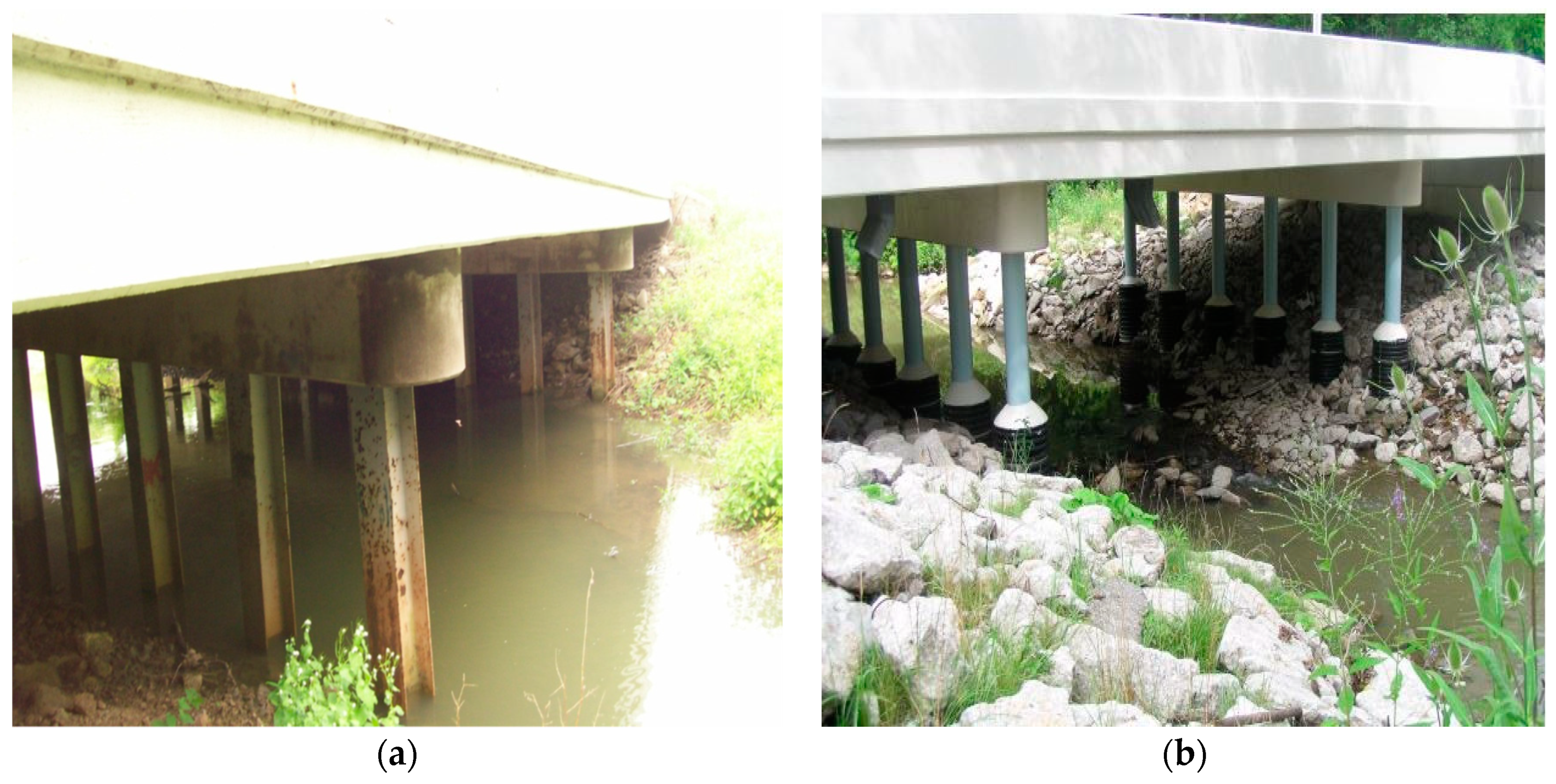Therefore, T-type piers is not typically recommended, as it is very difficult to remove debris from them (ODOT Bridge Design Manual, 2007) [20]. Rather, H-pile and concrete pile piers will be appropriate choices in such conditions. Figure 1a shows typical H-piles used in Ohio bridges. Pier encasement is one of the rehabilitation methods often used to allow the reuse of existing pile piers during the repair, where an existing pile pier is enclosed with a polyethylene or PVC pipe large enough to provide at least three inches of concrete cover over the existing pier when filled. One-inch wide stainless steel bands are also wrapped around the pipe at one-foot spacing and are tightened enough to prevent any elongation during placing of concrete into the pipe. Figure 1b shows typical H-piles after encasement.

2.2. Modeling Approach

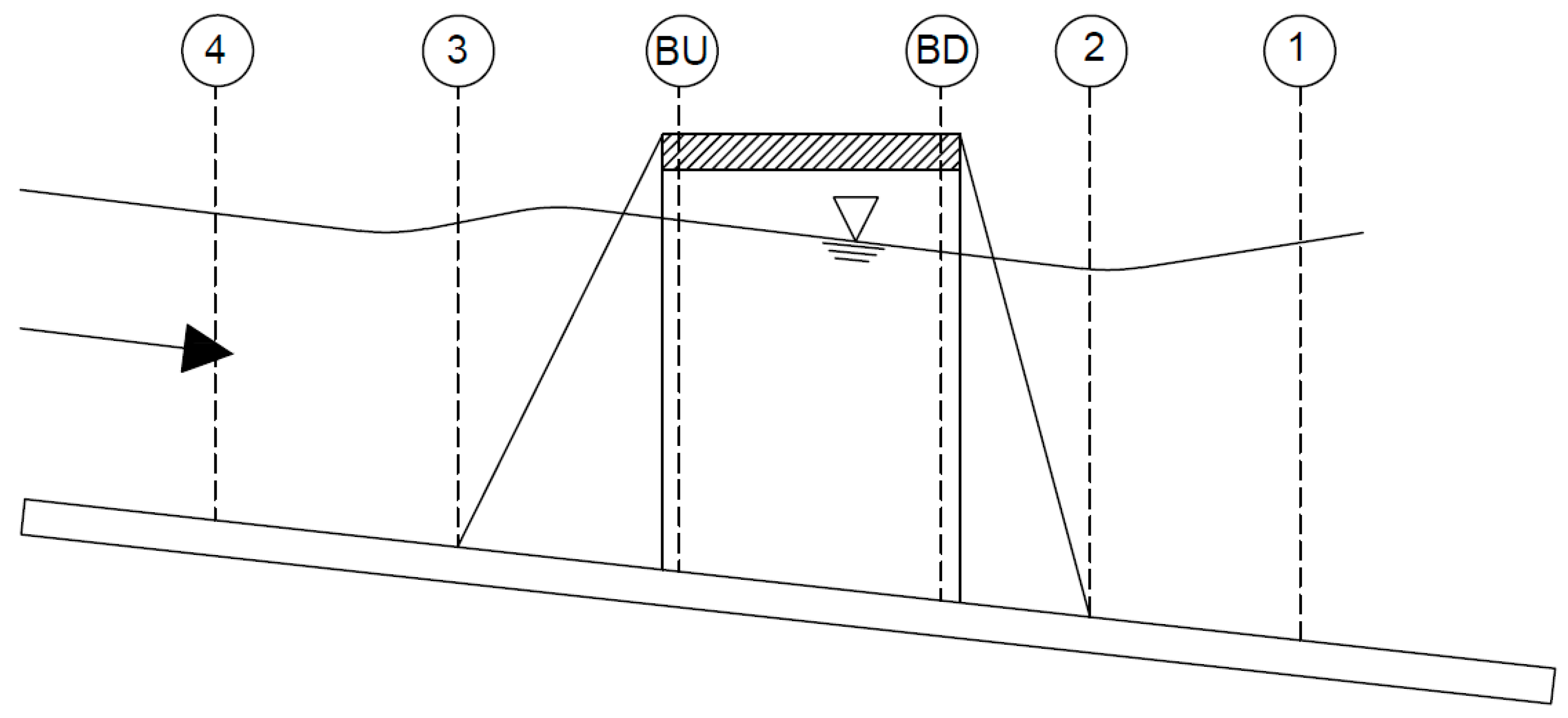
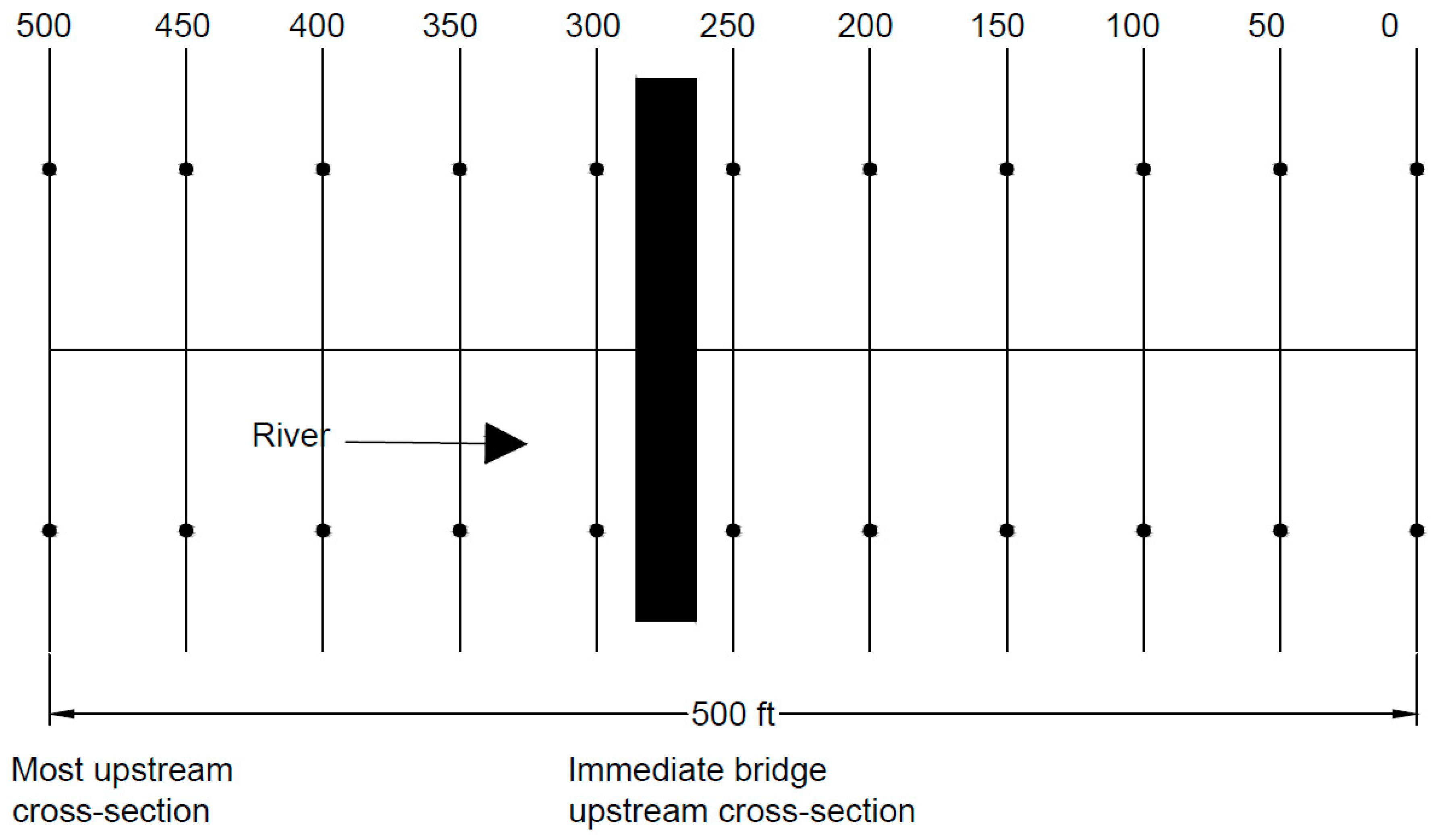
HEC-RAS is one of the most widely used tools for hydraulic simulation near the bridge site to evaluate the backwater effects, mainly due to its accuracy in modeling natural streams with negligible cost [21]. It uses four cross-sections: Upstream and downstream of the pier from the centerline of the channel for hydraulic analysis near the bridge site [18]. Figure 2 shows typical channel profile and cross-section locations. Cross-section 1 is located sufficiently downstream from the structure, whereas Cross-section 2 is located slightly downstream of the bridge (downstream toe of the embankment). Cross-section 3 is commonly placed at the upstream toe of the embankment. However, Cross-section 4 is the farthest upstream of the bridge, where the flow lines are approximately parallel, and the cross-section is fully effective. The contraction length (Lc) is referred to as the distance between Cross-section 3 and Cross-section 4, and the expansion length (Le) is referred to as the distance between Cross-section 1 and Cross-section 2. Typically, the Lc is less than Le, and should be determined by field investigations during high flows. Generally, Lc is adopted as the average obstruction length, and Le is typically determined after field investigation, which depends on the degree of constriction, slopes, and roughness of overbank/channel. Once an expansion ratio is selected, it will be multiplied by Lc to determine Le.

HEC-RAS offers a few options for water surface profile computations. One of the methods generally used for water surface profile computation is an equation suggested by Yarnell [22]. Yarnell developed an empirical equation based on 2600 experiments, which were conducted on large channels. Yarnell did not include all possible pier shapes in his experiment. Rather, his experiments mostly relied on rectangular and trapezoidal piers. Since his equation was developed mainly for specific conditions, this method may not be applicable unless the case study falls within the scope of his experiments. Moreover, the equation is sensitive to the pier shape coefficient, area of obstruction and velocity of water [23], but not sensitive to the shape of bridge opening, bridge abutment, and the width of the bridge. Therefore, this method is only used if the energy loss is particularly important due to piers [23].

The energy and momentum methods are the most physically based methods and suitable for various flow conditions. However, both methods have some limitations. For example, the energy method takes into account the loss through the contraction and expansion, but not the losses due to the shape of the pier. The momentum method considers the losses due to drag forces in the pier, but this method calculates the weight using an average bed slope, which is practically not possible to compute for natural cross-sections.

Since the goal of this research was to investigate the effect of pier encasement on the rise in headwater elevations, high-flow computations in HEC-RAS were implemented either using the standard step method or by using separate hydraulic equations for pressure/weir flow. In pressure and weir flow methods, HEC-RAS automatically uses the suitable type of equations based on the flow situation. For example, HEC-RAS uses two types of orifice flow depending upon the flow condition: (i) When only the upstream side of the bridge section is in contact with the water; and (ii) when the bridge constriction is flowing completely full [18]. In summary, the following methods should be used for high-flow regimes.

• The energy method should be used in case the bridge deck is a small obstruction to the flow and the bridge opening is not behaving as a pressurized orifice.
• The pressure and weir method could be an appropriate choice when the bridge deck and the road embankment create a significant obstruction to the flow.

The energy-based method should be selected if the bridge is significantly submerged and flow over the road is not behaving like a weir flow. The momentum method should be selected in case the significant drag losses can be expected near the pier.

3. Material and Methodology

3.1. HEC-RAS Model Inputs

All channel and pier configurations were run in non-encased and encased conditions for comparison assuming the flow was contained within the channel geometry. The study was conducted using typical trapezoidal cross-sections of the river. The study was limited to only two kinds of piers: H-piles and round concrete pile piers. Moreover, the shape of pier encasement to be provided was round. The pier encasement data to be incorporated into the HEC-RAS analysis were adopted using ODOT document shown in

Table 2. Pile pier and encasement data provided by ODOT.

Run	Existing Size	Shape	Existing Type	Encasement	Type	Shape
1	12″	Square	H-Pile	24″ ID/28″ OD	PE	Round
2	16″ OD	Round	Concrete Pile	30″ ID/36″ OD	PE	Round

. Multiple numbers of piers with varying shapes (circle and square) were modeled in HEC-RAS, and a parametric study was performed by analyzing pre- and post-encasement water surface elevations under varying channel configurations. The generic flat bottom channel section with 2:1 side slopes and the Manning’s roughness coefficient (n) of 0.035 were considered for all the channel configurations. The drag coefficient constant for circular and square pier were taken as 1.2 and 2, respectively. In addition, the model was developed for each nine different bottom widths varying from 20 to 180 ft at 20 ft interval for the various river slope conditions, such as 0.3%, 0.5%, 0.7%, and 1.0%. For the same geometric configuration, the simulation was conducted using two and three pier rows by maintaining a minimum span of 18 ft and a maximum span of 58 ft between two piers. This limited the use of pier numbers depending upon the size of the channel width in consideration. For example, for a smaller channel bottom width, such as 20 ft, two piers were sufficient. However, the bigger bottom channel width, such as 140, 160, and 180 ft, could accommodate three piers. The flow discharge was chosen according to the channel carrying capacity, which ranged from 200 to 20,000 cfs.

3.2. Model Establishment

A flat bottom generic channel section of side slope 2:1 with varying widths and number of piers (two and three) was developed in HEC-RAS in order to see the effect of bridge pier encasement on water surface level. Since HEC-RAS requires a minimum of four cross-sections for the simulation of water surface level near the bridge, numerous cross-sections were developed by creating two cross-sections at first and then interpolating them equally into certain numbers depending upon the reach length. The suitable reach length was adopted based on the width of the channel bottom in consideration. For example, reach length of 500 ft was considered for channel bottom width of 180 ft and decreased subsequently as the channel width was decreased. The typical channel cross-section in HEC-RAS with 180 ft bottom width is shown in Figure 3.

Similarly, the location of immediate upstream and upstream site of the bridge for various reach lengths under consideration is shown in

Table 3. Reach length and location from the center line of the bridge.

Channel Bottom Width (ft)	Number of Piers	Number of Cross-Sections	Reach Length (ft)	Most Upstream from Center Line of Bridge (ft)	Immediate Upstream from Center Line of Bridge (ft)
20	2	10	250	125	13.88
40	2, 3	10	250	125	13.88
60	2, 3	10	300	150	16.66
80	2, 3	10	300	150	16.66
100	2, 3	11	400	180	30
120	2, 3	11	450	205	25
140	3	11	450	205	25
160	3	11	500	225	25
180	3	11	500	225	25

.

Water surface elevations were computed using energy equation (standard step method) available in HEC-RAS model. Two piers were used for the channel of 20 ft bottom width, whereas analysis was accomplished using both two and three piers separately for channel bottom widths of 40 to 120 ft. Similarly, three piers were used from 140 to 180 ft channel bottom width in order to maintain ODOT’s typical recommended distance between two piers (minimum 18 ft and maximum 58 ft span). Initial flow was provided for producing a depth of 3 to 10 ft for the specific channel geometry of two-pier row and three-pier row configurations. The flow volume was increased at 200 cfs increments up to the maximum possible flow that could be practically accommodated by the given channel size. This resulted in 224 various models including both encased and non-encased pier conditions. Figure 3 shows one such example of a model of bottom width 180 ft with several channel cross-sections. Similarly, Figure 4 shows the bridge cross-section with the pier location in the channel of 180 ft bottom width.

4. Results

The difference in water surface elevation for existing and proposed pier encasements for various channel widths and slopes were calculated exclusively by standard step method in HEC-RAS using a mixed flow regime even though experiments were conducted with the momentum and Yarnell method. The data were documented for both no-rise and rise conditions. Different states in the U.S. define the range of no-rise and rise conditions depending upon the allowable surcharge limit of flood.

Table 4. Allowable state surcharge limits as of 2003 [8].

State	Surcharge (ft)
Illinois	0.1
Indiana	0.1
Michigan	0.1
Minnesota	0.5
Montana	0.5
New Jersey	0.2
Ohio	0.5
Wisconsin	0
All other states	1

shows that the allowable state surcharge limits of 0.5 ft as the no-rise condition for the State of Ohio. Therefore, this threshold of 0.5 ft was used for each channel configuration to identify the no-rise and rise conditions.

Table 5. No-rise condition for the circular pier.

Serial No	Bottom Channel Width (ft)	Flow Range (cfs)	Number of Piers	Slope (%)	Most Upstream Cross-Section	Immediate Bridge Upstream Cross-Section
					Flow (cfs)	Flow (cfs)
1	20	200–5600	2	0.3	Flow ≤ 5600	Flow ≤ 5600
				0.5	Flow ≤ 2400	Flow ≤ 1800
				0.7	Flow ≤ 1400	Flow ≤ 800
				1	Flow ≤ 1400	Flow ≤ 800
2	40	200–8400	2	0.3	Flow ≤ 8400	Flow ≤ 8400
				0.5	Flow ≤ 8400	Flow ≤ 6800
				0.7	Flow ≤ 7600	Flow ≤ 4400
				1	Flow ≤ 3800	Flow ≤ 2600
			3	0.3	Flow ≤ 8400	Flow ≤ 8200
				0.5	Flow ≤ 3600	Flow ≤ 2600
				0.7	Flow ≤ 4000	Flow ≤ 2400
				1	Flow ≤ 2200	Flow ≤ 1400
3	60	200–11,400	2	0.3	Flow ≤ 11,400	Flow ≤ 11,400
				0.5	Flow ≤ 11,400	Flow ≤ 11,400
				0.7	Flow ≤ 8600	Flow ≤ 5400
				1	Flow ≤ 7800	Flow ≤ 5400
			3	0.3	Flow ≤ 11,400	Flow ≤ 11,400
				0.5	Flow ≤ 8200	Flow ≤ 6400
				0.7	Flow ≤ 5200	Flow ≤ 3200
				1	Flow ≤ 5000	Flow ≤ 3200
4	80	200–13,400	2	0.3	Flow ≤ 13,400	Flow ≤ 13,400
				0.5	Flow ≤ 13,400	Flow ≤ 13,400
				0.7	Flow ≤ 12,400	Flow ≤ 8200
				1	Flow ≤ 9800	Flow ≤ 8200
			3	0.3	Flow ≤ 13,400	Flow ≤ 13,400
				0.5	Flow ≤ 13,400	Flow ≤ 9800
				0.7	Flow ≤ 8200	Flow ≤ 5400
				1	Flow ≤ 7800	Flow ≤ 5400
5	100	200–15,000	2	0.3	Flow ≤ 15,000	Flow ≤ 15,000
				0.5	Flow ≤ 15,000	Flow ≤ 15,000
				0.7	Flow ≤ 15,000	Flow ≤ 14,000
				1	Flow ≤ 11,400	Flow ≤ 10,600
			3	0.3	Flow ≤ 15,000	Flow ≤ 15,000
				0.5	Flow ≤ 15,000	Flow ≤ 15,000
				0.7	Flow ≤ 13,800	Flow ≤ 8600
				1	Flow ≤ 9800	Flow ≤ 6000
6	120	200–20,000	2	0.3	Flow ≤ 20,000	Flow ≤ 20,000
				0.5	Flow ≤ 20,000	Flow ≤ 20,000
				0.7	Flow ≤ 20,000	Flow ≤ 20,000
				1	Flow ≤ 13,200	Flow ≤ 16,800
			3	0.3	Flow ≤ 20,000	Flow ≤ 20,000
				0.5	Flow ≤ 20,000	Flow ≤ 20,000
				0.7	Flow ≤ 20,000	Flow ≤ 20,000
				1	Flow ≤ 14,200	Flow ≤ 8800
7	140	200–20,000	3	0.3	Flow ≤ 20,000	Flow ≤ 20,000
				0.5	Flow ≤ 20,000	Flow ≤ 20,000
				0.7	Flow ≤ 20,000	Flow ≤ 19,000
				1	Flow ≤ 17,000	Flow ≤ 15,200
8	160	200–20,000	3	0.3	Flow ≤ 20,000	Flow ≤ 20,000
				0.5	Flow ≤ 20,000	Flow ≤ 20,000
				0.7	Flow ≤ 20,000	Flow ≤ 17,600
				1	Flow ≤ 18,200	Flow ≤ 20,000
9	180	200–20,000	3	0.3	Flow ≤ 20,000	Flow ≤ 20,000
				0.5	Flow ≤ 20,000	Flow ≤ 20,000
				0.7	Flow ≤ 20,000	Flow ≤ 20,000
				1	Flow ≤ 20,000	Flow ≤ 20,000

shows no-rise condition for the circular pier using two and three piers for all channel configurations for the ranges of flow that each channel could accommodate. For example, a 20 ft channel bottom width with a bed slope of 0.3% and two piers showed no-rise condition for flow range up to 5600 cfs at the immediate upstream cross-section of the bridge. Similar condition (no-rise condition) was observed in most upstream cross-section for the flow range up to 5600 cfs. The flow was limited to 5600 cfs, as it was the maximum discharge that the channel could accommodate. Multiple analyses were conducted for other channel slopes including 0.5%, 0.7%, and 1%. Analyses indicated that the rise condition would be realized for higher slopes even if smaller flows are considered. For example, rise condition would be experienced for 2400 cfs and 1400 cfs flows for the channel with bed slopes of 0.5% and 0.7%, respectively (Table 5).

For a channel of 40 ft bottom width with the slope of 0.3%, no-rise condition was detected up to the flow range of 8400 cfs. This was true regardless the number of piers (two and three) that had been chosen. Similarly, for a channel bottom width of 40 ft and the longitudinal slope of 0.5% (two piers), no-rise condition was experienced for the flow up to 8400 cfs at the most upstream cross-section and for the flow up to 6800 cfs at the immediate bridge upstream. The flow was limited to 8400 cfs, as it was the maximum discharge that could be occupied by the channel of 40 ft bottom width. As the slope was increased, the rise condition was realized even for the relatively lesser flows. For example, for 0.7% and 1% channel slopes with two piers bridge system, the rise condition was experienced for flows greater than 7600 cfs and 3800 cfs, respectively. The detail ranges of the flows for no-rise condition for various channel configurations were reported in Table 5. Any values exceeding the flow ranges that were reported in Table 5 for the respective channel configurations would produce the rise condition.

Similarly,

Table 6. No-rise condition for the square pier.

Serial No	Bottom Channel Width (ft)	Flow Range (cfs)	Number of Piers	Slope (%)	Most Upstream Cross-Section	Immediate Bridge Upstream Cross-Section
					Flow (cfs)	Flow (cfs)
1	20	200–5600	2	0.3	Flow ≤ 5600	Flow ≤ 5600
				0.5	Flow ≤ 2600	Flow ≤ 1600
				0.7	Flow ≤ 1800	Flow ≤ 1000
				1	Flow ≤ 1600	Flow ≤ 1000
2	40	200–8400	2	0.3	Flow ≤ 8400	Flow ≤ 8400
				0.5	Flow ≤ 7800	Flow ≤ 6200
				0.7	Flow ≤ 8400	Flow ≤ 5000
				1	Flow ≤ 4200	Flow ≤ 3000
			3	0.3	Flow ≤ 8400	Flow ≤ 8400
				0.5	Flow ≤ 3800	Flow ≤ 2800
				0.7	Flow ≤ 4800	Flow ≤ 2600
				1	Flow ≤ 2600	Flow ≤ 1800
3	60	200–11,400	2	0.3	Flow ≤ 11,400	Flow ≤ 11,400
				0.5	Flow ≤ 11,400	Flow ≤ 11,400
				0.7	Flow ≤ 9400	Flow ≤ 5800
				1	Flow ≤ 7200	Flow ≤ 4600
			3	0.3	Flow ≤ 11,400	Flow ≤ 11,400
				0.5	Flow ≤ 8400	Flow ≤ 6400
				0.7	Flow ≤ 6000	Flow ≤ 4600
				1	Flow ≤ 4800	Flow ≤ 2800
4	80	200–13,400	2	0.3	Flow ≤ 13,400	Flow ≤ 13,400
				0.5	Flow ≤ 13,400	Flow ≤ 13400
				0.7	Flow ≤ 13,400	Flow ≤ 9000
				1	Flow ≤ 8800	Flow ≤ 7200
			3	0.3	Flow ≤ 13,400	Flow ≤ 13,400
				0.5	Flow ≤ 13,400	Flow ≤ 13,400
				0.7	Flow ≤ 8200	Flow ≤ 5000
				1	Flow ≤ 7600	Flow ≤ 4800
5	100	200–15,000	2	0.3	Flow ≤ 15,000	Flow ≤ 15,000
				0.5	Flow ≤ 15,000	Flow ≤ 15,000
				0.7	Flow ≤ 15,000	Flow ≤ 13,800
				1	Flow ≤ 10,400	Flow ≤ 12,200
			3	0.3	Flow ≤ 15,000	Flow ≤ 15,000
				0.5	Flow ≤ 15,000	Flow ≤ 15,000
				0.7	Flow ≤ 14,800	Flow ≤ 11,600
				1	Flow ≤ 13,600	Flow ≤ 9200
6	120	200–20,000	2	0.3	Flow ≤ 20,000	Flow ≤ 20,000
				0.5	Flow ≤ 20,000	Flow ≤ 20,000
				0.7	Flow ≤ 20,000	Flow ≤ 20,000
				1	Flow ≤ 14,200	Flow ≤ 19,000
			3	0.3	Flow ≤ 20,000	Flow ≤ 20,000
				0.5	Flow ≤ 20,000	Flow ≤ 20,000
				0.7	Flow ≤ 20000	Flow ≤ 20,000
				1	Flow ≤ 14,800	Flow ≤ 13,200
7	140	200–20,000	3	0.3	Flow ≤ 20,000	Flow ≤ 20,000
				0.5	Flow ≤ 20,000	Flow ≤ 20,000
				0.7	Flow ≤ 20,000	Flow ≤ 17,200
				1	Flow ≤ 15,200	Flow ≤ 17,600
8	160	200–20,000	3	0.3	Flow ≤ 20,000	Flow ≤ 20,000
				0.5	Flow ≤ 20,000	Flow ≤ 20,000
				0.7	Flow ≤ 20,000	Flow ≤ 20,000
				1	Flow ≤ 18,200	Flow ≤ 20,000
9	180	200–20,000	3	0.3	Flow ≤ 20,000	Flow ≤ 20,000
				0.5	Flow ≤ 20,000	Flow ≤ 20,000
				0.7	Flow ≤ 20,000	Flow ≤ 20,000
				1	Flow ≤ 20,000	Flow ≤ 20,000

shows a no-rise in water surface elevation for square piers for two- and three-pier cases for all channel configurations. The rise in water surface elevation was significantly affected by the pier width as the rise in water surface elevation was clearly noticeable with the increase in pier width. Since the increased pier width further creates the obstruction to the flow, it is not surprising to see such increase in the water surface elevation. Moreover, the effect was significant for smaller channel width and greater slope relative to bigger channel width and lesser slope.

The rise in water surface elevation was also greatly affected by the flow volume in the river cross-section. For example, the difference in water surface elevation for existing (before encasement) and proposed pier (after encasement) for the channel section of 20 ft and 1.0% slope was much lesser for 200 cfs (0.02 ft) when compared to flow volume 5000 cfs (0.98 ft). This was mainly because the higher flow volume occupied more channel area; therefore, even a small obstruction to its flow made a significant change. In general, the water surface elevations after the encasement were found to be slightly increased depending upon the flow volume under consideration. This modest increase in water surface elevation was noticeable for higher flow volume compared to lower flow volume.

The slope of a channel section also greatly influenced the water surface elevation. For example, the difference in water surface elevation for existing and proposed pier encasement for the 20 ft channel section was greatly affected by channel slope even for the same discharge. For example, a 0.3% channel slope with the discharge of 5000 cfs showed a lesser rise in water surface elevation (0.23 ft) when compared to the slope of 0.7% and 1.0% (0.88 and 0.98 ft, respectively). Typically, the differences in water surface elevation were higher for 0.7% and 1.0% slopes when compared to 0.3% channel slope, indicating that the steeper channel could produce higher water surface elevation compared to flatter slopes.

Channel bottom width was another parameter in the channel configuration, which affected the water surface elevation. For example, the difference in water surface elevation for existing and proposed pier for the channel section of 20 ft bottom width with 1.0% channel slope and 5000 cfs flow showed a greater rise in water surface elevation (0.98 ft). However, for a channel of 180 ft bottom width with the same channel section properties and flow volume (5000 cfs), the rise in water surface elevation was significantly less (0.01 ft).

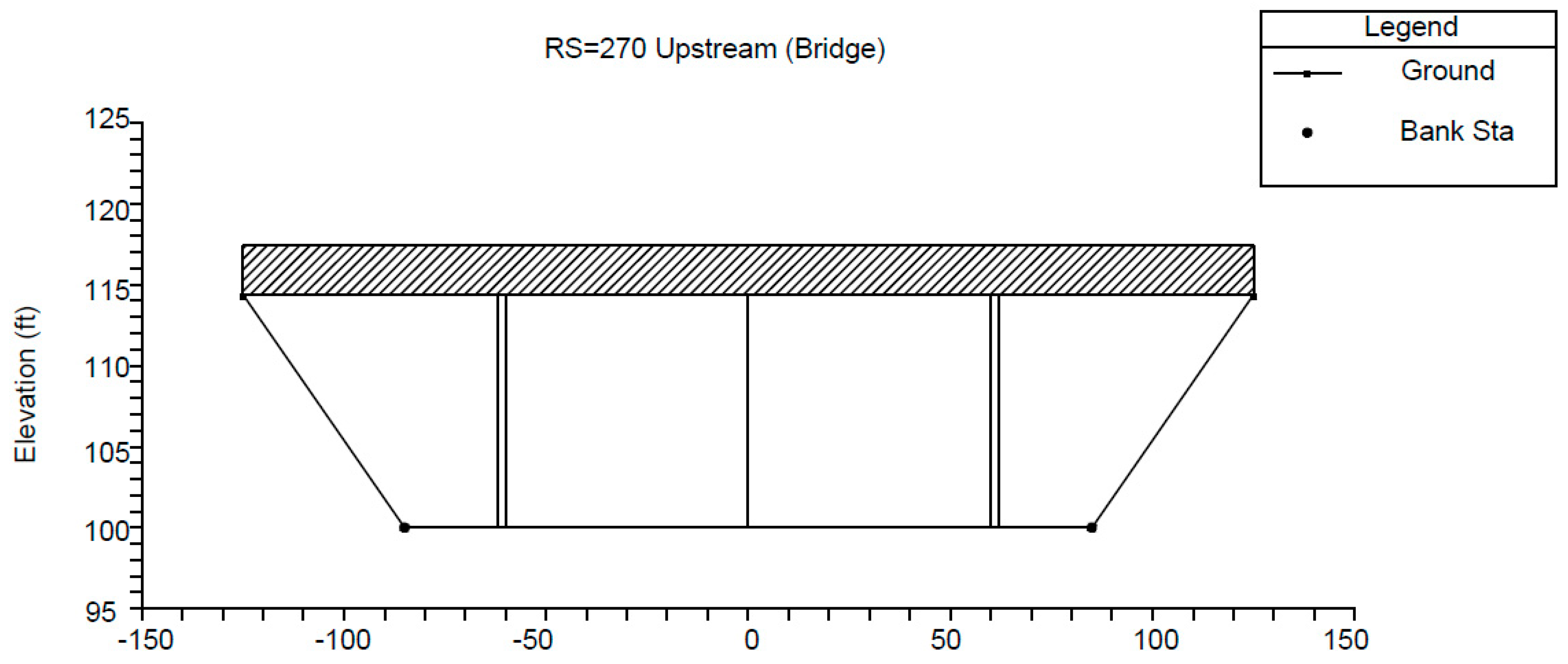
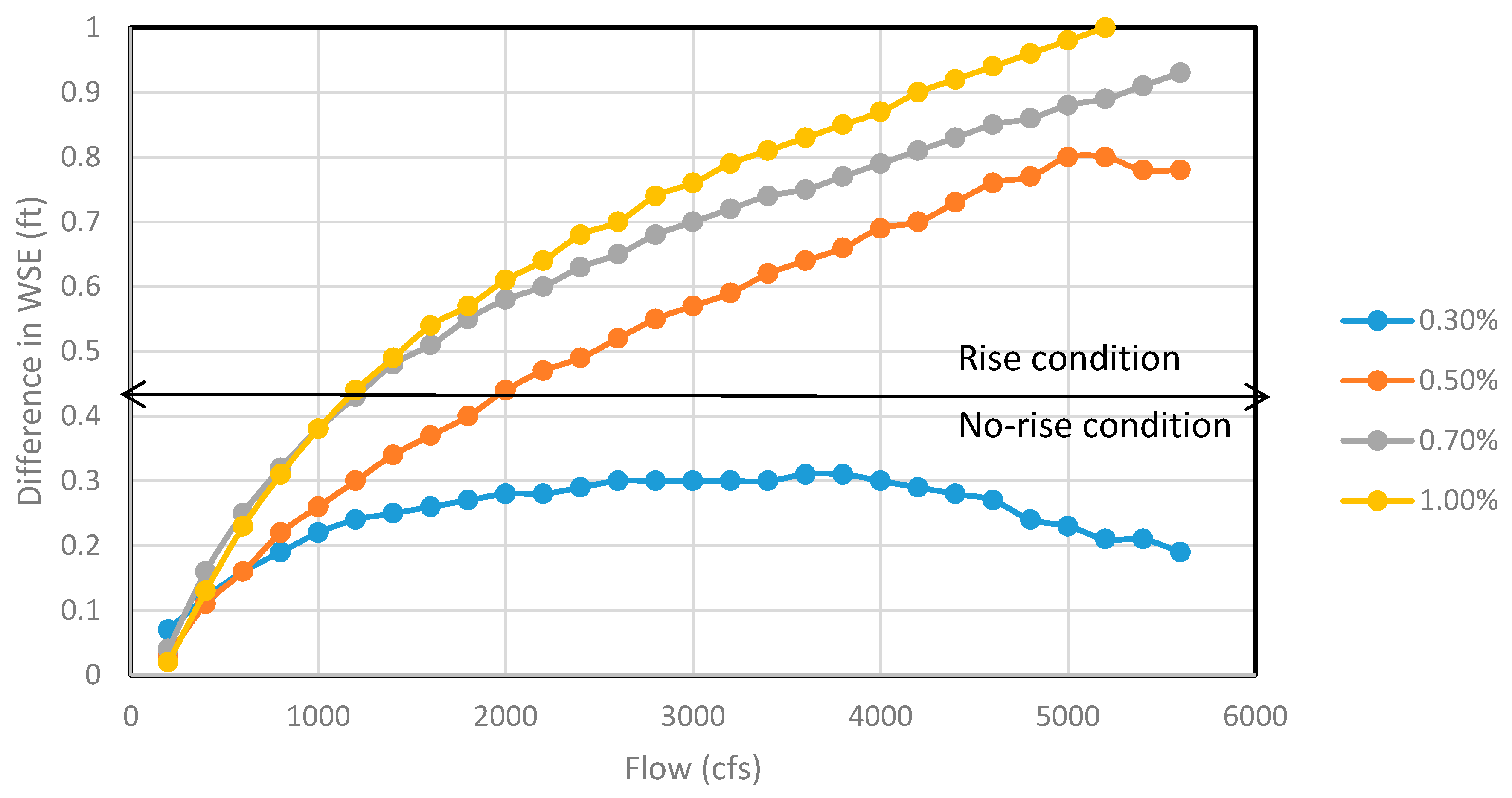
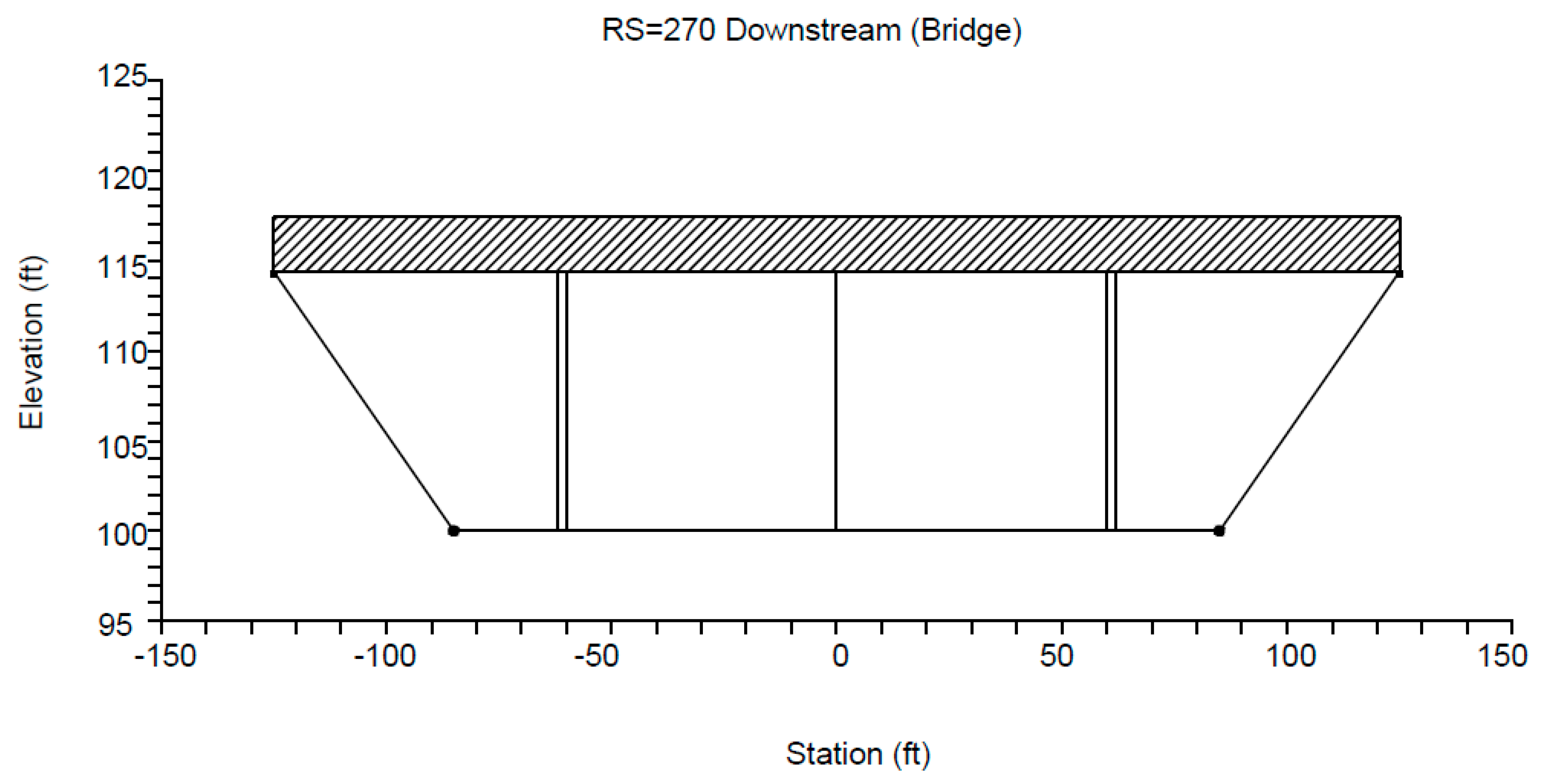
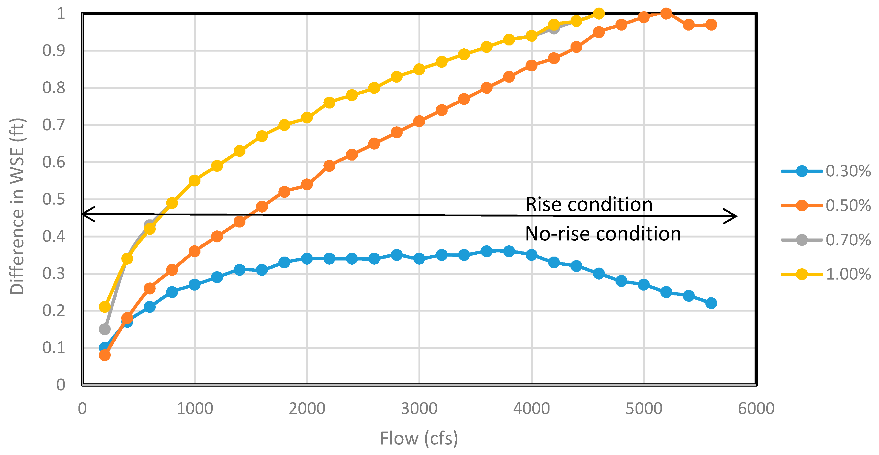
HEC-RAS also generates profile plots displaying the water surface elevation, energy gradeline, critical depth, bank stations, etc. Figure 5 shows the difference in water surface elevation at most bridge upstream for all the flows (200–5600 cfs) for 20 ft bottom width with two circular piers for four channel slopes. The channel section with 0.3% slope showed no-rise for all the possible flow ranges. As the slope was increased, rise condition started to appear. For example, the rise condition was detected at 2400 cfs with 0.5% slope, whereas the rise condition was observed shortly after 1400 cfs for both 0.7% and 1% slopes. Figure 6 shows the difference in water surface elevation at the immediate bridge upstream for the 20 ft channel section for all flow volumes. Similar trend was detected with 0.3% channel slope indicating no-rise conditions for all flow volumes. However, it started increasing gradually as the slope was progressively increased. For example, the rise condition appeared for 0.5% slope at flows greater than 1800 cfs, whereas the rise condition appeared for 0.7% and 1.0% slopes at flows greater than 800 cfs.

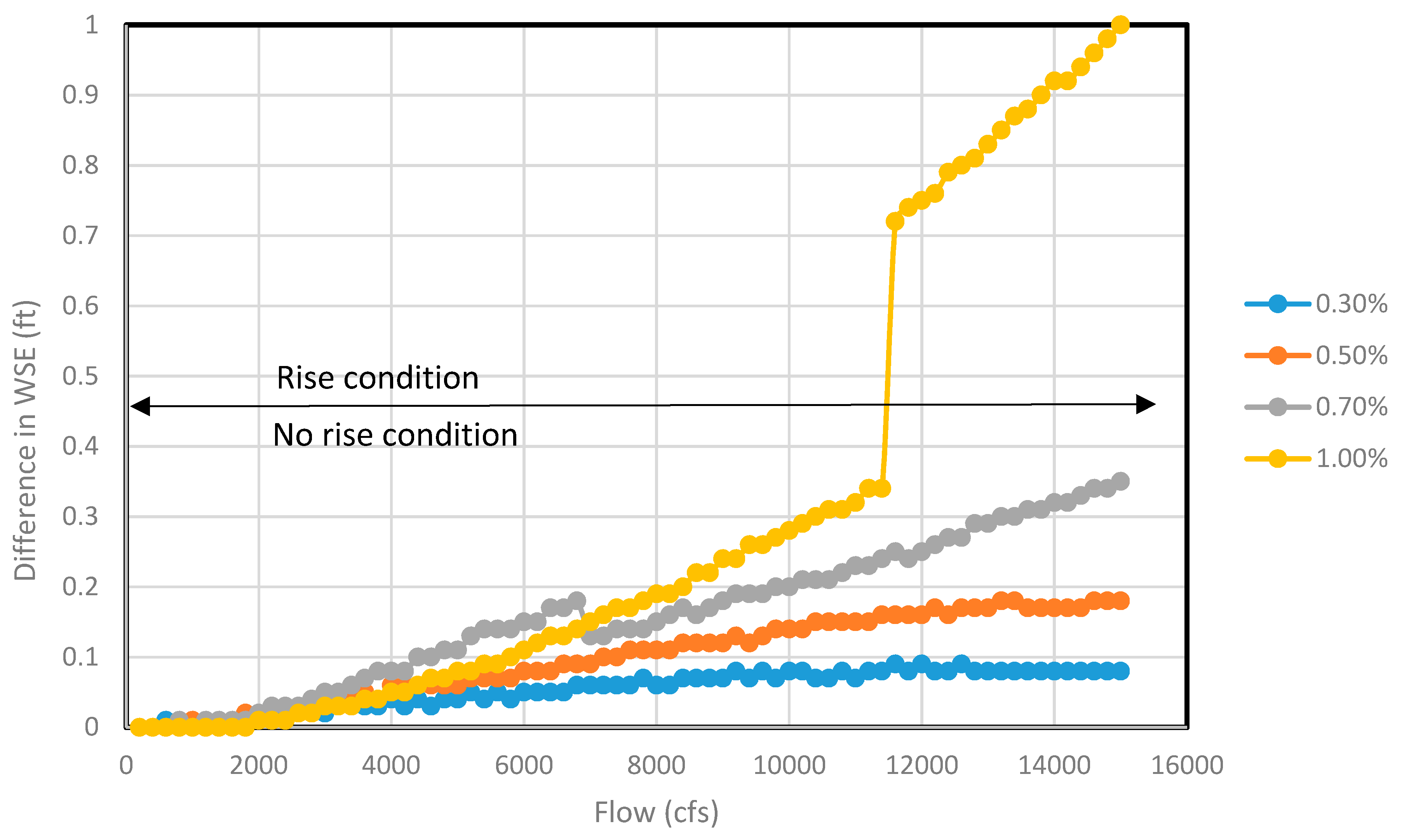
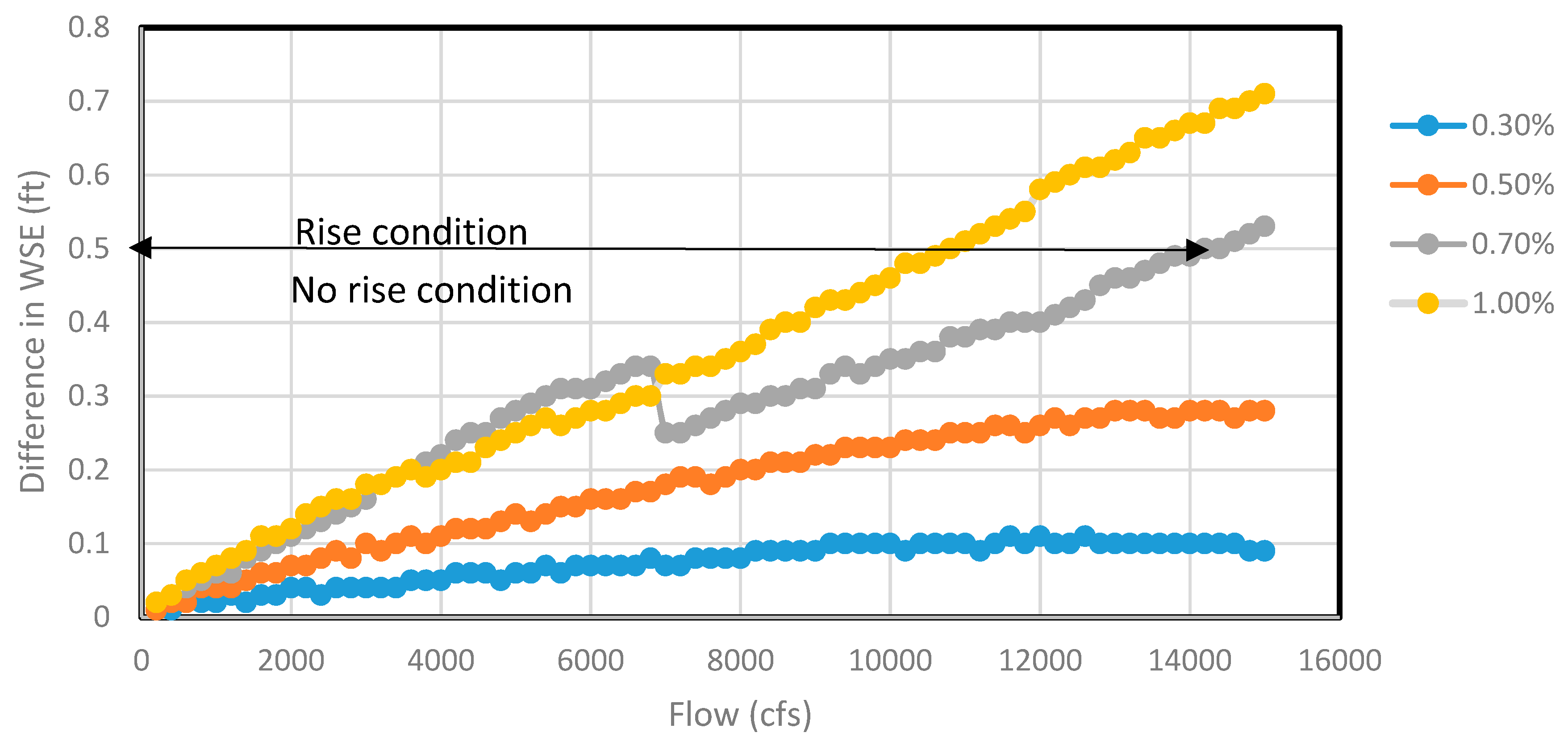
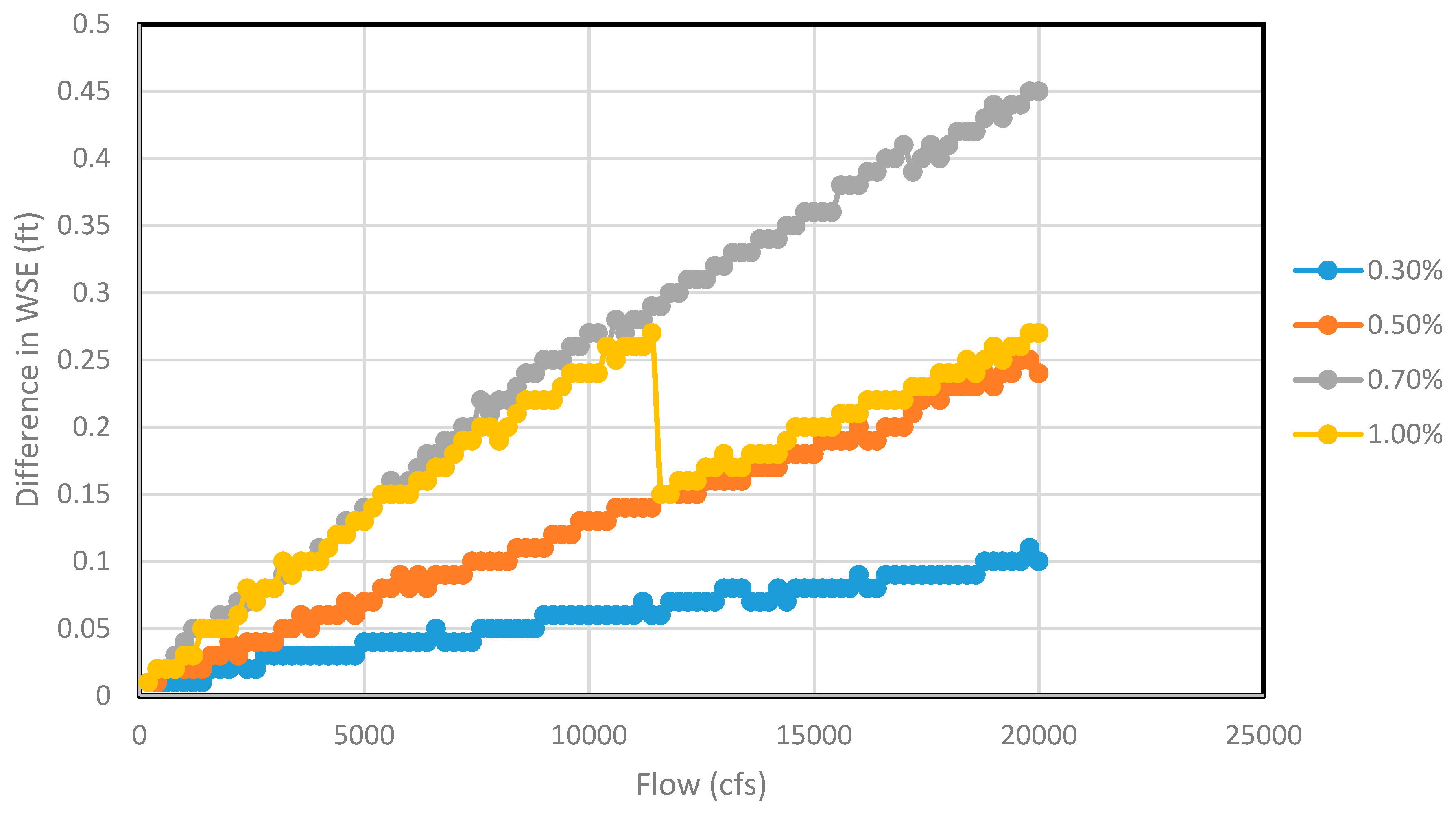
Figure 7 shows the difference in water surface elevation at most bridge upstream for all flow ranges (200—15,000 cfs) for 100 ft bottom width with two circular piers. It covers all four channel slopes considered for the analysis. Channel sections with 0.3%, 0.5%, and 0.7% slopes showed no-rise for all possible flow ranges. However, as the slope was increased to 1.0%, rise condition started to appear. When flow was increased from 11,400 to 11,600 cfs, there was an abrupt rise from 0.32 to 0.72 ft and later the same gradual increasing trend continued. Figure 8 shows the difference in water surface elevation at immediate bridge upstream for the same channel section for all flow ranges. The trend remained similar with 0.3% and 0.5% slopes showing no-rise for all flow ranges. However, as the slope was increased, the rise condition appeared for 0.7% and 1.0% slopes for higher flow rates after 14,000 cfs and 10,600 cfs, respectively.

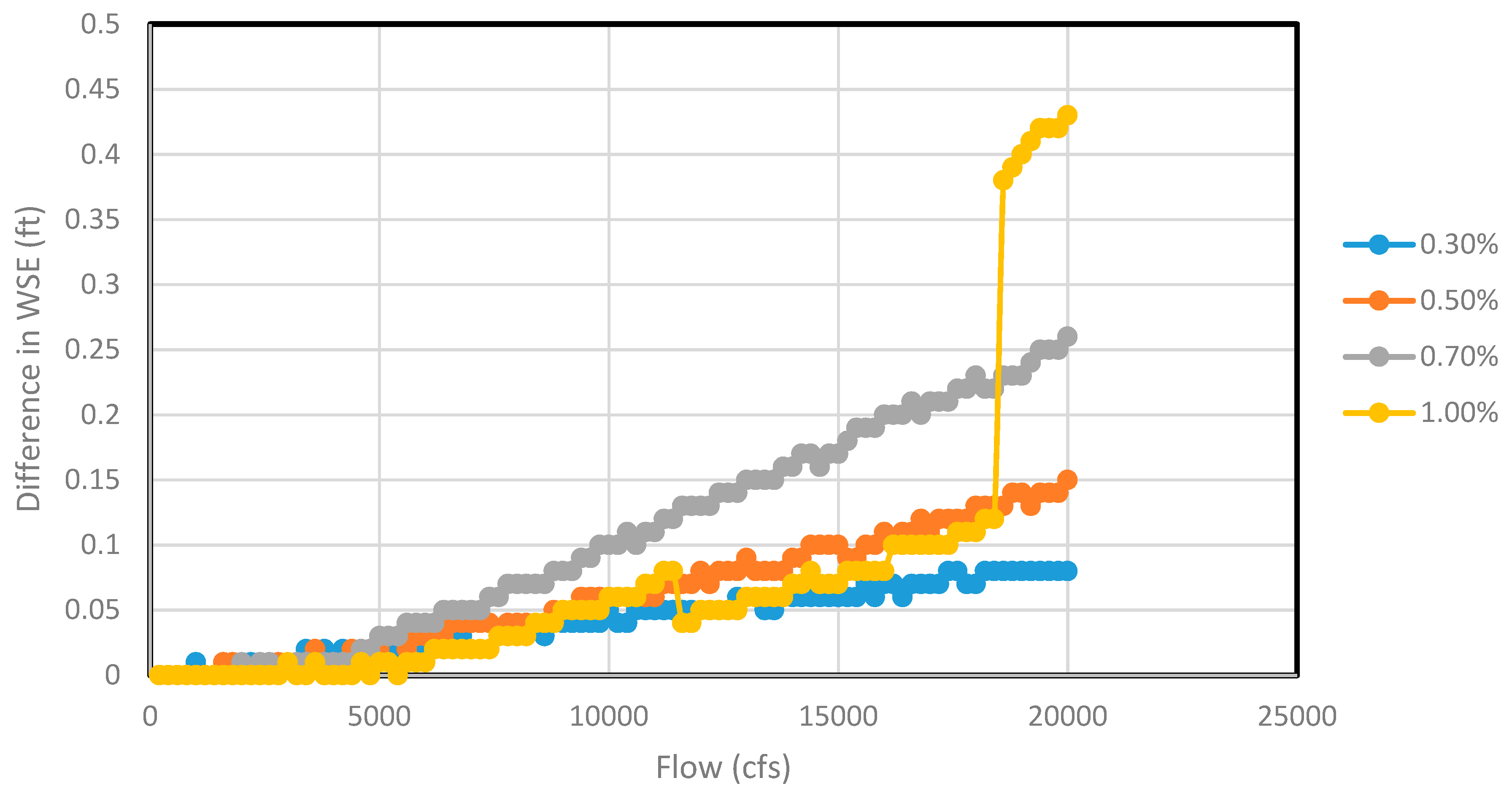
Figure 9 and Figure 10 show the difference in water surface elevation at most bridge upstream and immediate bridge upstream, respectively, for all flow ranges (200—20,000 cfs) for the channel section of 180 ft bottom width comprising three circular piers. It showed a no-rise condition in both cross-sections for all flow ranges regardless of the channel slopes. For the conciseness of the manuscript, the graphical plots of water surface elevation versus flows for all channel widths were not reported. However, the rise condition and no-rise condition for each channel configurations have been tabulated. Table 5 shows the no-rise condition for the circular pier, whereas Table 6 shows the no-rise condition for the square pier. The rise condition will be experienced for all flows exceeding the flow limits specified in Table 5 and Table 6.

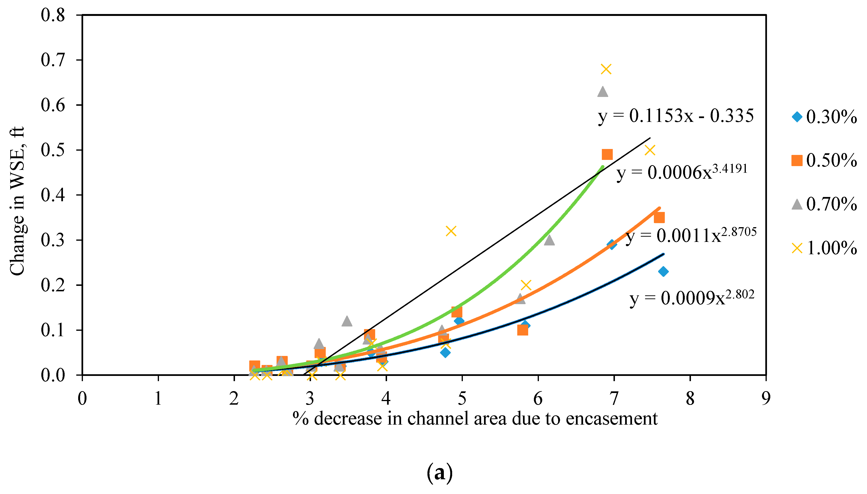
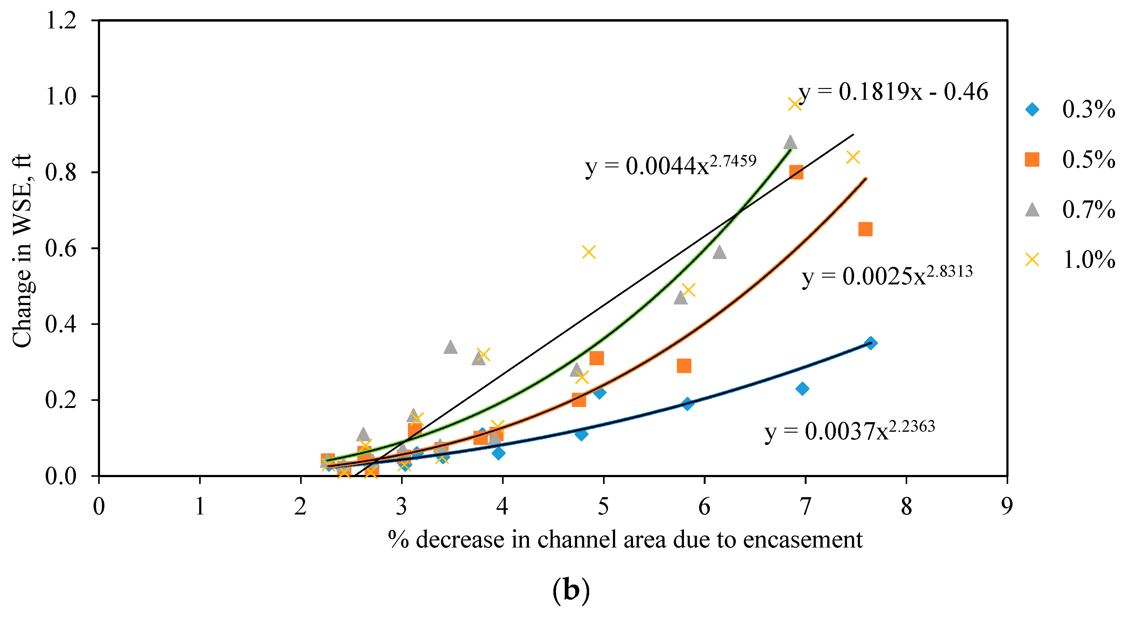
The analysis indicated that there was an increase in water surface elevation after encasement due to the increase in discharge. In addition, increased slope also produced a greater rise in water surface elevation after the encasement. The study suggested that the channel of 180 ft bottom width did not show any rise in water surface elevation even with the maximum discharge. Moreover, even the higher slope did not have any substantial effect on water surface elevation in a wider channel. In general, wider channels provided bigger volume for water flow. Therefore, the obstruction in such channels showed relatively lesser water surface elevation. Typically, no-rise conditions were prevalent in wider channels, whereas the rise conditions were observed in narrower channels. In addition, higher slope and greater discharge increased the water surface elevation after the encasement. Since rise in water surface elevation was typically due to decrease in effective flow area between piers, it was of interest to see the relationship of change in water surface elevation with percentage decrease in the channel area. However, all flow conditions did not contribute to the rise condition. Similarly, 20 ft channel width could not accommodate the flow more than 5600 cfs. Therefore, selected were two flow conditions (2400 cfs and 5000 cfs) to identify the relationship between percentage decrease in the channel area and the rise in water surface elevation. For 2400 cfs, all channels started showing some changes in water surface due to pier encasement. Similarly, selected channel with a flow of 5000 cfs was selected for simplicity as this flow could be accommodated by all channel widths. Figure 11a,b show the change in water surface elevation per unit percentage decrease in the channel area for 2400 cfs and 5000 cfs flow, respectively. It is interesting to note that a generic form of power equation, such as Y = aX^b, could represent such a relationship for most slopes except for 1%. For the 1% channel slope, linear equation best fitted the data.

The proposed equations to estimate the rise conditions for each percentage reduction in area is tabulated in

Table 7. The generic equation proposed to estimate the increased water surface elevation with reduced area for two flow conditions (2400 cfs and 5000 cfs).

Flow = 2400 cfs
Slopes	Proposed Equation	R2
0.30%	Y = 0.0009x2.802	0.909
0.50%	Y = 0.0011x2.8705	0.842
0.70%	Y = 0.0006x3.4191	0.845
1%	Y = 0.115–0.335	0.79
Flow = 5000 cfs
Slopes	Proposed Equation	R2
0.30%	Y = 0.0037x2.236	0.909
0.50%	Y = 0.0025x2.831	0.894
0.70%	Y = 0.0044x2.746	0.801
1%	Y = 0.819x − 0.46	0.887

.

These results were reported using the standard step method, while other computational methods, such as Momentum and Yarnell methods, were also used to see the effect of pier case encasement in water surface elevation (not shown). However, no significant difference was observed in the result for various methods. In fact, the pattern of rise and no-rise conditions obtained using standard step method was comparable with that obtained from other methods, such as momentum and Yarnell methods.

5. Summary and Conclusions

The rise in water surface elevation may create problems in bridge piers located at high-risk flood zones after any pier encasement. In this study, HEC-RAS software was utilized to test and implement the different encasement scenarios. For every channel, four models were constructed using four different slopes (0.3%, 0.5%, 0.7%, and 1.0%). Each channel configuration was modeled twice: One without pier encasement (existing) and the other with pier encasement (proposed). Therefore, 224 models with different channel configurations and number of piers were modeled and water surface elevations were determined. Finally, it was found that the increase in water surface elevation after pier encasement was a function of the width of the pier, flow volume, channel slope, and channel bottom width.

With encasement, the pier width increased resulting in the further constriction of the channel and increased water surface elevation. The effect was significant for smaller bottom widths and steeper channel slopes. With the increase in the channel slope, there was a rise in the water surface elevation regardless of the channel width. For example, the steeper channel slopes, such as 0.7% and 1.0%, showed the maximum rise in water surface elevation after the pier encasement even for smaller flow rate. On the other hand, channels with flatter slopes, such as 0.3% and 0.5%, showed relatively lesser rise in water surface elevation after pier encasement. Moreover, the bottom width of a channel had a vital effect on water surface elevation. For wider channels, the rise in water surface elevation after the pier encasement was nominal. For example, the channel with a bottom width of 180 ft showed negligible rise in water surface elevation after the pier encasement. This was true even for steeper slopes (0.7% and 1.0%). Whereas for channels with smaller bottom width, the rise in water surface elevation after the pier encasement was significant. For example, the channel with a bottom width of 20 ft showed a rise in water surface elevation than that of a width of 180 ft after the pier encasement. In addition, flow volumes also had a substantial effect on increased water surface elevation, which was clearly noticeable after the pier encasement.

Furthermore, the difference in water surface elevations for existing and proposed pier configurations was computed for all the channel sections. The computed difference was broadly categorized into the rise and no-rise conditions depending upon the simulated water surface level in the upstream section of the bridge. The rise and no-rise condition were identified following standards in the State of Ohio, which considers a no-rise condition if the increase in water surface elevation is limited to 0.5 ft. Since the rise in water surface elevation is due to the decrease in the effective flow area in the channel, the increase in water surface elevation was plotted with the percentage decrease in flow area. A generic power equation in the form of Y = aX^b was developed for most channel slopes, where Y represent the rise in water surface elevation and X represents the percentage decrease in the channel area.

Finally, this study will be beneficial and will serve as a guideline for rehabilitation practices, such as bridge pier encasement in flood prone areas. The study also shows the effect of slopes, flow volumes, and channel bottom widths on water surface elevation after the pier encasement, which might be very helpful for concerned government agencies to take necessary protections in highly flood prone zones.