A Correlation–Scale–Threshold Method for Spatial Variability of Rainfall

Abstract

Rainfall data at fine spatial resolutions are often required for various studies in hydrology and water resources. However, such data are not widely available, as their collection is normally expensive and time-consuming. A common practice to obtain fine-spatial-resolution rainfall data is to employ interpolation schemes to derive them based on data available at nearby locations. Such interpolation schemes are generally based on rainfall correlation or distance between stations. The present study proposes a combined rainfall correlation-spatial scale-correlation threshold method for representing spatial rainfall variability. The method is applied to monthly rainfall data at a resolution of 0.25° × 0.25° latitude/longitude across Australia, available from the Tropical Rainfall Measuring Mission (TRMM 3B43 version). The results indicate that rainfall dynamics in northern and northeastern Australia have far greater spatial correlations when compared to the other regions, especially in southern and southeastern Australia, suggesting that tropical climates generally have greater spatial rainfall correlations when compared to temperate, oceanic, and continental climates, subject to other influencing factors. The implications of the outcomes for rainfall data interpolation and the rain gauge monitoring network are also discussed, especially based on results obtained for ten major cities in Australia.

1. Introduction

Rainfall data at fine spatial (and temporal) resolutions are crucial for a variety of studies in hydrology and water resources, including for flow/flood forecasting, soil erosion estimation, and water quality modeling, among others. However, fine-resolution spatial rainfall data are not widely available in many parts of the world, especially in developing and under-developed regions. An important reason for this is that installing rain gauges at fine spatial resolutions is costly and time-consuming. Although recent advances in remote sensing technology (e.g., satellites, radars) have facilitated hydrometeorologic measurements at fine resolutions, such measurements still require the “ground truth” (e.g., rain gauge data) for deriving rainfall values and, hence, rainfall estimation is subject to a wide range of uncertainties.

In the absence of rainfall measurements at fine spatial resolutions, studies normally resort to interpolation schemes for obtaining rainfall at such resolutions based on rainfall measurements available at one or more nearby locations. The last century has witnessed numerous studies on spatial rainfall variability, rain gauge monitoring network design, development and applications of rainfall interpolation methods, and the associated uncertainties [1,2,3,4,5,6,7,8,9,10,11,12,13,14].

The above studies have significantly advanced our understanding of spatial (and temporal) rainfall variability and our ability to estimate rainfall at fine spatial resolutions. Although estimation of rainfall at fine spatial (and temporal) resolutions continues to be tremendously challenging, thanks to the vagaries of its dynamics, these studies and their outcomes certainly provide important insights into potential areas for further improvements. The availability of new/better rainfall measurement technology and more advanced scientific concepts also provides additional opportunities to advance research. For instance, (1) more accurate estimation of rainfall at certain scales is now possible through merging satellite/radar products and rain gauge measurements [15,16,17,18]; and (2) renewed and fresh insights into theories of complexity, nonlinear dynamics, scaling, and pattern recognition offer new avenues for studying the dynamics of rainfall [10,19,20,21,22].

Despite these advances in studying the spatial (and temporal) variability of rainfall, some important issues in the existing approaches still remain. For instance, (1) geographically nearby points are generally assumed to be more correlated (and connected) than distant points; (2) correlation between points is often the basis for assessing connectedness, with only limited consideration for scale, threshold, etc.; and (3) smoothing of data often takes priority in estimation at ungauged locations. All of these factors lead to various uncertainties in rainfall estimation.

We attempt to address these issues in the present study, with Australia as a case study area. More specifically, we propose an approach that combines rainfall correlation, spatial scale, and correlation threshold. In doing so, we also take advantage of the availability of rainfall data at equal spatial resolutions (grids), rather than just using the rainfall data from ground-based rain gauges. Here, we consider the TRMM 3B43 dataset, which is a combined product of rainfall observed through TRMM (Tropical Rainfall Measuring Mission) and other satellites as well as gridded rain gauge data [23,24]. We consider (1) different spatial scales to assess if and how rainfall correlations vary with scale and (2) different correlation thresholds to evaluate if and how rainfall correlations vary with respect to threshold.

The rest of this paper is organized as follows: In Section 2, the methodology used for calculating spatial rainfall correlations with respect to scale and threshold is described. In Section 3, details of the study area and data considered are reported. Section 4 presents the analysis and results for Australia-wide data and also for ten major cities. Section 5 offers some implications of the results and scope for further research.

2. Methodology

Figure 1 presents a simplified schematic representation of the spatial rainfall variability and estimation problem, studied here. The figure shows that a given area can be represented by a number of equal-size (or unequal) cells (“grids”). Given that rainfall data are available for all/some grids (“gauged grids”), the problem then is (1) to assess the spatial rainfall variability in the area and (2) to derive rainfall data for the other grids (“ungauged grids”), based on some criteria. In this study, we address the first problem and propose a method that combines three different properties relevant to spatial rainfall variability: rainfall correlation (“similarity”), spatial scale (“neighborhood”), and correlation threshold (“significance”). The method is explained next.

Let us consider any particular grid, denoted by i, in the study area, as shown in Figure 1. The grid i will have a certain number of “neighborhood” grids, denoted by j. The number of neighborhood grids will vary depending upon both the “location” of the grid i and the “spatial extent” (or size) of the neighborhood (e.g., the larger the scale of the neighborhood, the greater the number of grids). If there is only one neighborhood grid, the rainfall correlation between grids i and j (i.e., C_i,j) is simply given by

C_i,j = Corr(R_i, R_j)

(1)

where R_i and R_j are the rainfall values (as a time series) at grids i and j, respectively. Equation (1) can be extended or generalized to any number of neighborhood grids j = 1, 2, 3, …, N − 1, where N is the total number of grids (including grid i) within the spatial extent of the neighborhood considered.

The spatial extent of the neighborhood and, thus, the number of neighborhood grids can be chosen in various ways, ranging from a careful consideration of the hydroclimatic, topographic, and other properties to a purely arbitrary manner. Here, we adopt the idea of “scale” for choosing the number of neighborhood grids. A particular advantage of this idea is that it maintains, for a given scale, an equal number of grids in all directions with respect to grid i. The use of scale is also highly appropriate for equal-size grid-based data, such as those provided by TRMM.

With this, our analysis of spatial rainfall involves increasing (or decreasing) the scale of the neighborhood of grid i and evaluating its effects on rainfall correlations between grid i and respective grids j. We call these different scales “box sizes” or “window sizes” (n). For any grid i, we first consider different box sizes corresponding to different numbers of neighborhood grids (n = 1, 2, 3, and so on), but equal in all directions for any given number; for illustration, box sizes of 1 (with total number of grids N = 9, including grid i), 2 (25 grids), and 3 (49 grids), are shown in Figure 1. For such a grid i, we then calculate the rainfall correlations C_i,j for all grids j in the respective box sizes. Based on these correlations, we determine the number of grids N′ having correlations greater than a prespecified threshold value (T) (where 0 ≤ T ≤ 1.0), and express it as a percentage of the total number of grids j for the respective box sizes (i.e., N − 1 grids in the respective box), as follows:

PC_i,n = (N′/(N − 1)) × 100

(2)

where PC_i,n is the percentage of grids for which the correlation is greater than threshold T. The procedure is repeated for each of the other grids.

3. Study Area and Data

In this study, spatial rainfall variability in Australia (see Figure 2) is studied. Australia’s climate and, hence, rainfall dynamics are significantly influenced by the hydroclimatic mechanisms that occur in the surrounding oceans. For instance, the El-Niño Southern Oscillation (ENSO), the western Pacific and Indian Ocean sea surface temperatures (SST), and the Southern Ocean atmospheric variability have varying degrees of influence on different regions of the country [25]. The climate varies from tropical in the north to arid (or desert) in the middle to temperate in the south; see Figure 2 for the climate division of Australia according to the Köppen climate classification and its modification [26,27]. Consequently, rainfall is highly variable in space (and time), and a large part of the country (especially the middle and the west) is dry. More than 80% of the country gets an annual rainfall of less than 600 mm, but the tropical region of the far north receives over 4000 mm.

Rainfall in Australia is mainly monitored by the Australian Bureau of Meteorology (BoM) using the thousands of rain gauges installed in different parts of the country; see Jeffrey et al. [28] for the locations of rain gauge stations in Australia. A large majority of these gauges covers only small regions, such as near the coasts of east, southeast, and southwest Australia, where much of the population is concentrated (in and around big cities). The number of rain gauges in the interior, which is largely desert and very sparsely populated, is very few. As for record length, some rain gauge stations have records for over 100 years, but some others have records for much shorter periods; in some stations, recording has already ended. A number of studies have studied the Australian rainfall data produced by the BoM and those derived based on them [10,17,22,24,28,29,30,31].

The launch of the Tropical Rainfall Measuring Mission (TRMM), a combined mission by the National Aeronautics and Space Administration (NASA) of the United States and the Japanese Aerospace Agency (JAXA), with an aim to measure tropical rainfall from space with combined passive and active microwave instruments [23], has allowed rainfall measurements at finer spatial (and temporal) resolutions across Australia (and other regions). The TRMM rainfall products are available at different levels of processing and also at different versions that reflect the improvements in the estimation algorithm since their launch [23,32]). Several studies have assessed the accuracy and uncertainties in TRMM rainfall data by comparing them with rain gauge (and other means of) observations in different regions around the world [13,32,33,34,35,36]. Some efforts have also been made to merge the TRMM rainfall data with rain gauge observations [15,16,17,37], including for Australia. Despite their uncertainties, the TRMM rainfall products have been used in many hydrologic applications [38,39,40]. Extensive details of the accuracy, uncertainties, merging, and use of the TRMM data are already available in the above studies (and in others) and, therefore, are not reported herein.

The rainfall data used in this study are from the TRMM 3B43 version. This version is a combined product of rainfall observed through TRMM and other satellites and gridded rain gauge data [23]. The rainfall data are available at a spatial resolution of 0.25° × 0.25° latitude/longitude and at the monthly scale. The data used here cover the period 1998–2007, the same period of data used in Woldemeskel et al. [17] in their effort to merge gauge and satellite rainfall with due consideration to the specification of uncertainty across Australia. In their study, Woldemeskel et al. [17] compared the TRMM data with high-quality rainfall data from 230 rain gauges across Australia. They found that the TRMM rainfall generally agreed with the rain gauge observations for much of Australia. Significant differences in statistical properties between the TRMM data and the ground rain gauge data were observed for only about 10% of the stations. It should be noted, however, that these stations are mainly located in the coastal areas where the rain gauge density is generally higher, but not in the interior regions where the rain gauge density is lower. This seems to imply that regions with low-density ground level rain gauges are not necessarily more vulnerable (than regions with high-density rain gauges) when it comes to uncertainties in TRMM rainfall data. Therefore, it may be reasonable to use the TRMM data for analysis even in regions where the rain gauge density is lower, such as in the interior of Australia. Nevertheless, despite its generally reliable nature, the TRMM 3B43 data set still has its own uncertainties due to various factors, including errors in remotely sensed data, ground-based data, and methodology in merging. Addressing this issue is beyond the scope of the present study. On the other hand, there exist even newer and better rainfall products, such as those from the Global Precipitation Measurement (GPM) mission, which may also be used in studies such as this. We will consider this in the future.

4. Analysis, Results, and Discussion

4.1. Analysis

We perform the analysis for all the 0.25° × 0.25° latitude/longitude grids across Australia. Recognizing (including through a preliminary analysis) that very small differences in distances (e.g., box sizes) do not significantly change the rainfall variability and also that far-off grids have almost no rainfall correlations (see below for details), we choose only a limited number of box sizes (n) for analysis (23, to be precise) to save time and computational resources. The box sizes we consider are n = 1 (3 × 3 = 9 grids), 2 (5 × 5 = 25 grids), 4, 6, 8, 10, 12, 14, 16, 18, 20, 22, 24, 26, 28, 30, 32, 34, 36, 38, 40, 42, and 44 (89 × 89 = 7921 grids). According to these, the distances considered for calculations vary from about 38 km to 1730 km, with approximately 80 km difference between every n considered (except between n = 1 and n = 2, in which case the distance is about 40 km). Further, to be consistent in the distance covered for all grids (on land), we also use data observed at relevant grids in the surrounding oceans on all sides (although this attempt is not completely successful, since data are not available beyond 50°S latitude). As for the threshold value (T), there is no definitive guideline for its selection. Here, we consider four different rainfall correlation thresholds: 0.5, 0.6, 0.7, and 0.8. The selection of these threshold values is largely based on our knowledge and experience with rainfall studies based on the concepts of complex networks [10,22,41]. We believe that this range of threshold values (0.5–0.8) is appropriate for monthly rainfall data, since most grids may have correlations exceeding 0.5, while only a very few grids may have correlations greater than 0.8. Therefore, selection of 0.5–0.8 will be more efficient and effective in the implementation of the study.

We find that the Australia-wide 0.25° × 0.25° grid analysis indeed provides some interesting results and interpretations on spatial rainfall variability against scale and correlation threshold. However, such are basically very general observations over a large region. Considering that rainfall dynamics in different regions in Australia are influenced by different hydroclimatic and topographic factors, it will be certainly more meaningful to study smaller regions for better interpretations. The fact that a majority of Australia’s population lives in a few major cities also emphasizes the need to study such areas. In view of these factors, we start with a brief presentation of the results for Australia-wide grids and then, on the basis of such results, discuss the results for ten major cities (i.e., ten different 0.25° × 0.25° grids in which the ten cities are situated) across Australia: Sydney, Melbourne, Brisbane, Perth, Cairns, Darwin, Hobart, Alice Springs, Adelaide, and Canberra (see Figure 2 for locations). The climates in these cities, according to the modified Köppen classification [26,27], are as follows: (1) Sydney: temperate—no dry season (hot summer); (2) Melbourne: temperate—no dry season (warm summer); Brisbane: subtropical (distinctly dry summer); Perth: temperate—moderately dry winter (hot summer); Cairns: tropical—rainforest (monsoonal); Darwin: tropical (savannah); Hobart: temperate—no dry season (mild summer); Alice Springs: grassland—hot (persistently dry); Adelaide: grassland—warm (persistently dry); and Canberra: temperate—no dry season (warm summer).

4.2. Results for Australia-Wide Analysis

Figure 3 presents some selected spatial rainfall correlations for the 0.25° × 0.25° grids across Australia. The plots correspond to box sizes (n) of 1 (3 × 3 = 9 grids), 6 (= 169 grids), 12 (= 625 grids), 18 (= 1369 grids), 24 (= 2401 grids), 30 (= 3721 grids), 36 (= 5329 grids), and 42 (85 × 85 = 7225 grids) and for a threshold value (T) of 0.6. The results reveal the following:

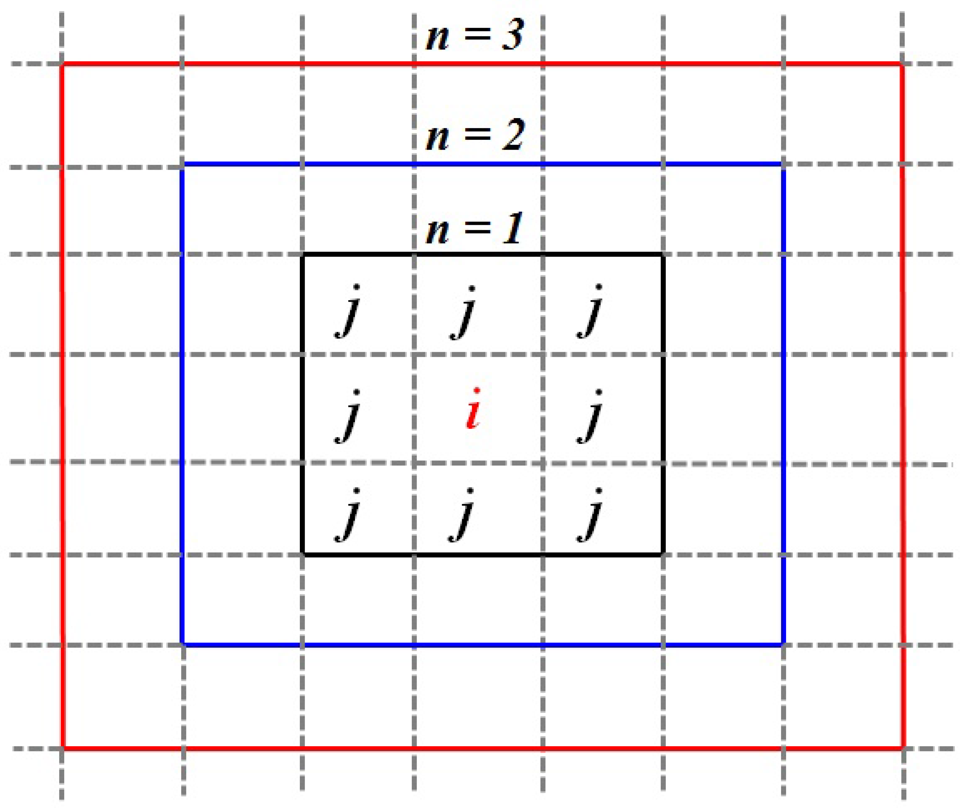
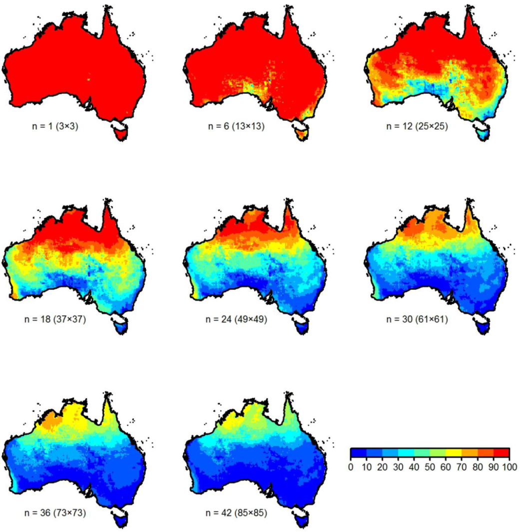
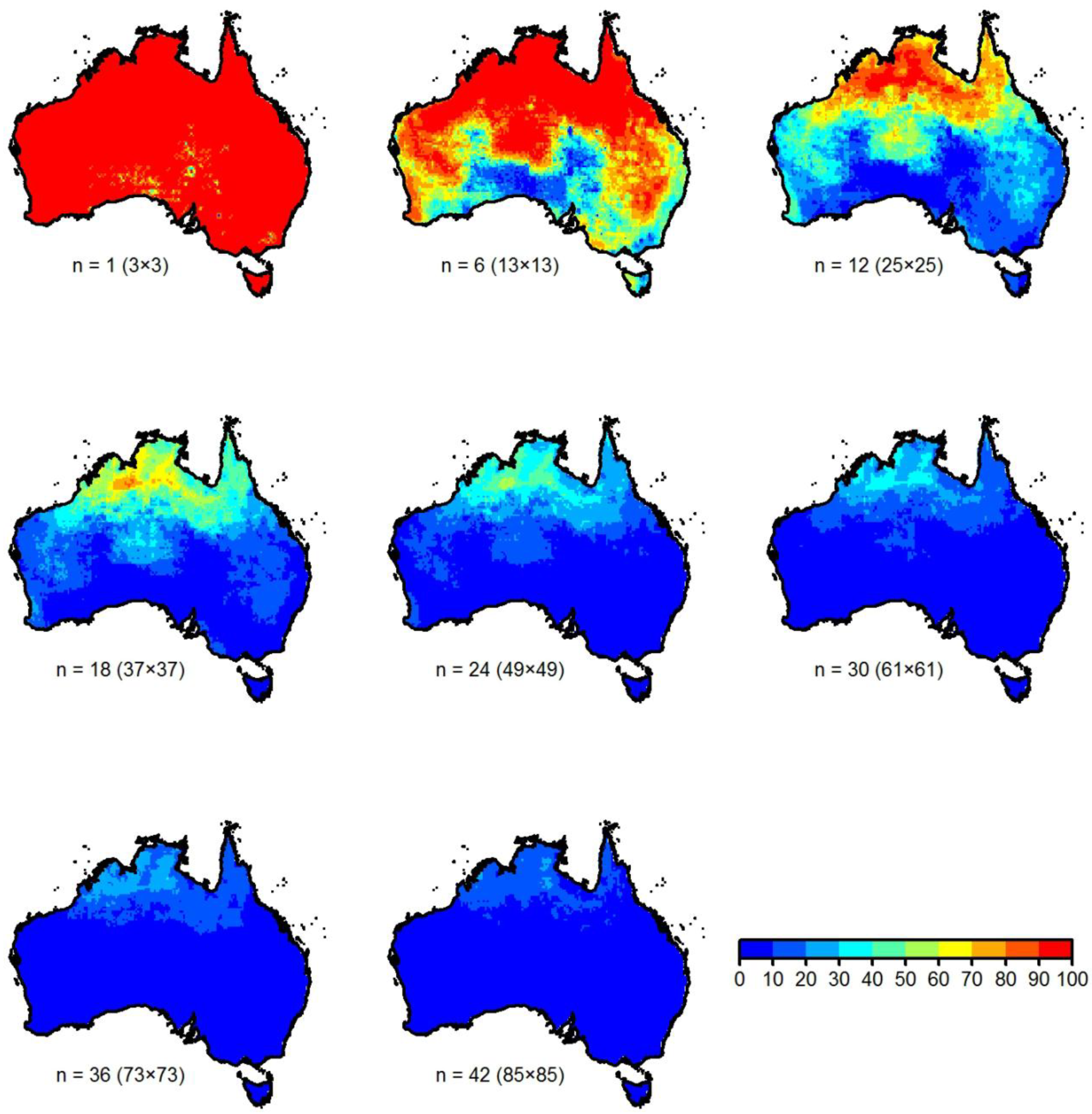
• When the box size is too small (e.g., n = 1), the spatial correlations are high all across Australia (i.e., almost all grids have rainfall correlations exceeding 0.6).
• When the box size is too large (e.g., n = 42), the spatial correlations are generally low (i.e., only 0–30% of grids have rainfall correlations exceeding 0.6), except in the northern region (where about 30–70% of grids have correlations exceeding T = 0.6).
• As expected, spatial rainfall correlation decreases as the box size increases (and vice versa) all across Australia. However, very clear changes are observed at/across certain box sizes, with “pockets of regions” having similar (or different) spatial correlations emerging; see, for instance, the changes in results for south and southeast Australia when n = 12 and for western Australia when n = 18 (when compared to those when n = 1).

Similar observations are also made for the other three threshold values (0.5, 0.7, and 0.8), subject to appropriate changes (e.g., percentage of grids exceeding a particular threshold, “pockets of regions”, and their areal extent). For instance, Figure 4 presents the results for T = 0.8, which is a much more stringent case when compared to T = 0.6.

4.3. Results for Ten Major Cities

For each of the ten cities, Figure 5 presents the spatial rainfall correlation results (expressed as a percentage of grids exceeding a given threshold, PC_i,n) for all the 23 box sizes (n, denoted by distance) and for all the four threshold levels (T) considered. The results generally indicate a decreasing PC_i,n against increasing n for any T, with saturation (in most cases) after a certain n. However, the manner in which PC_i,n decreases (e.g., trend and extent of change between successive n values) and the value of n at which it attains saturation are different for different thresholds for each city. In particular, the results for Perth, Cairns, and Darwin show significant differences in PC_i,n with respect to T, and those for Alice Springs, Adelaide, and Brisbane show noticeable differences. These results indicate that different cities exhibit different spatial rainfall correlations and variability and, thus, may require different interpolation schemes.

The above observation raises concerns about the application of a specific interpolation scheme for rainfall over a large region or nationwide. Further, since correlation thresholds have important implications for rainfall interpolation (including whether or not interpolation is necessary or effective), the results for any of the ten cities provide important clues as to the “distance of observation” one may deem appropriate for rainfall estimation at a point or “distance of estimation” one can confidently make based on available data. All these observations clearly suggest that spatial rainfall variability must be considered in terms of rainfall correlations, spatial scale, and correlation thresholds in a combined manner.

For still better comparisons and interpretations of the results among the ten cities, Figure 6 presents the results in a slightly different way, i.e., spatial rainfall correlations for all cities for a given threshold. The plots reveal that spatial rainfall correlations generally decrease with increasing box size (distance) for any correlation threshold, as expected. However, significant differences exist among the cities and are summarized as follows.

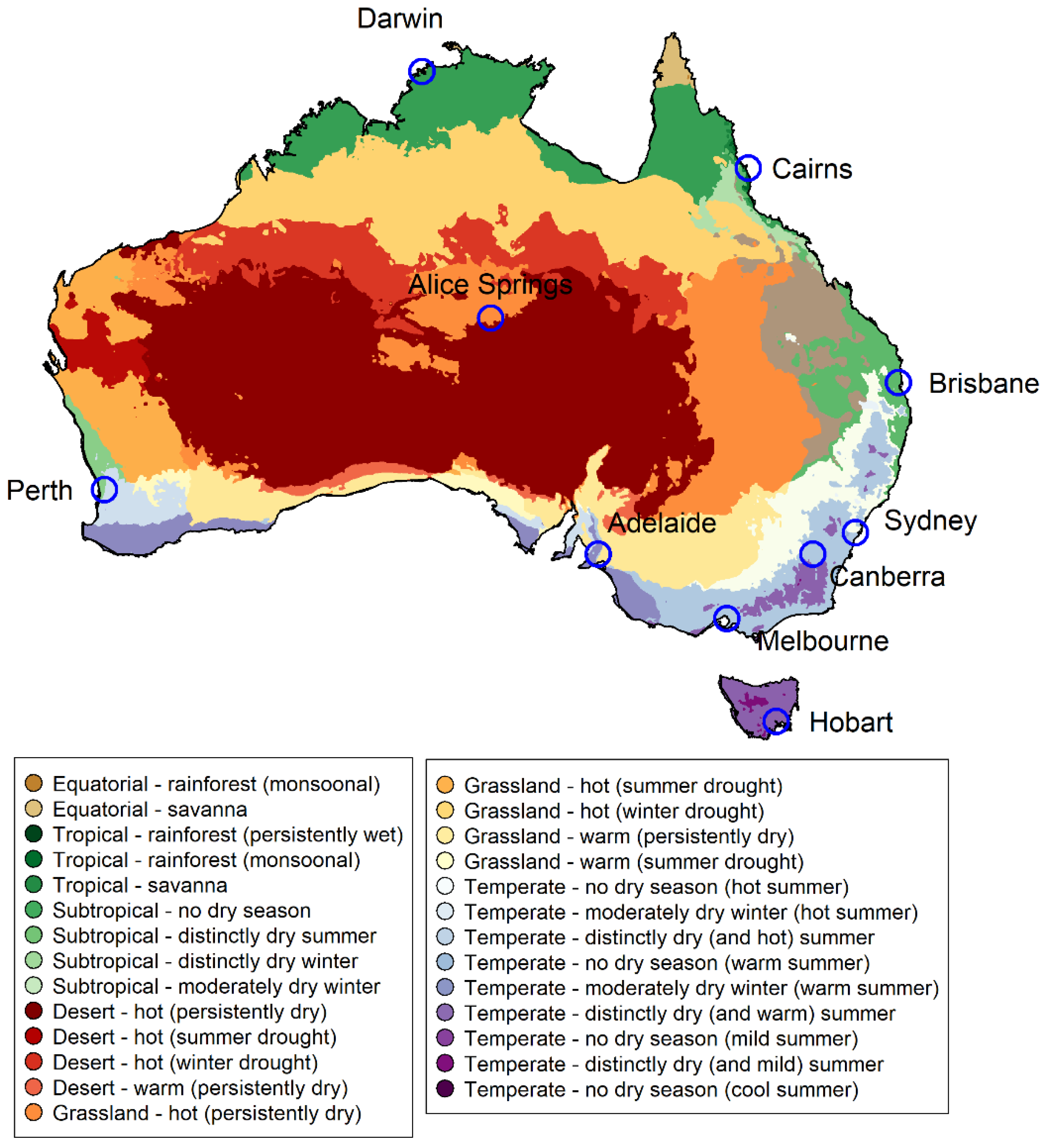
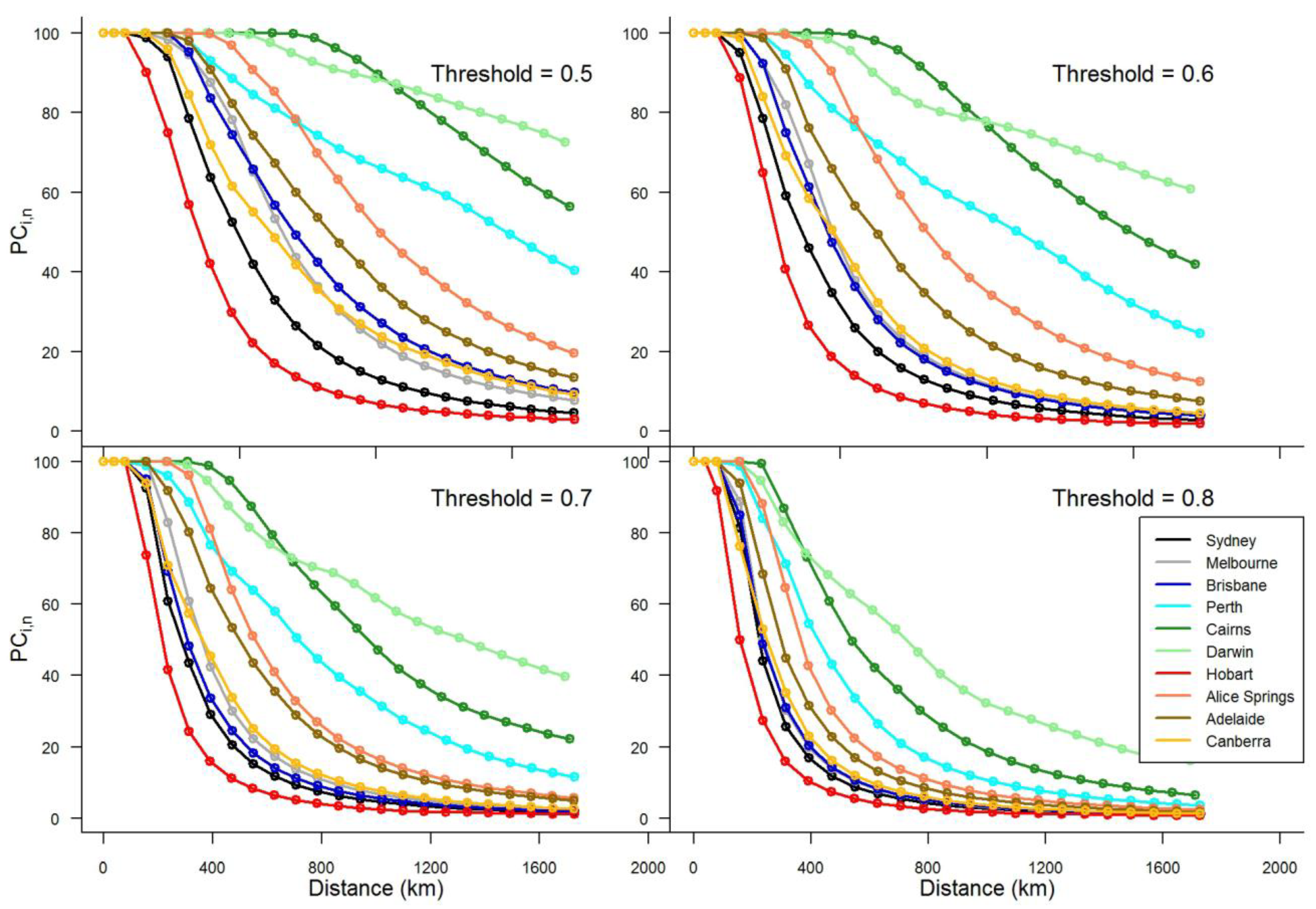
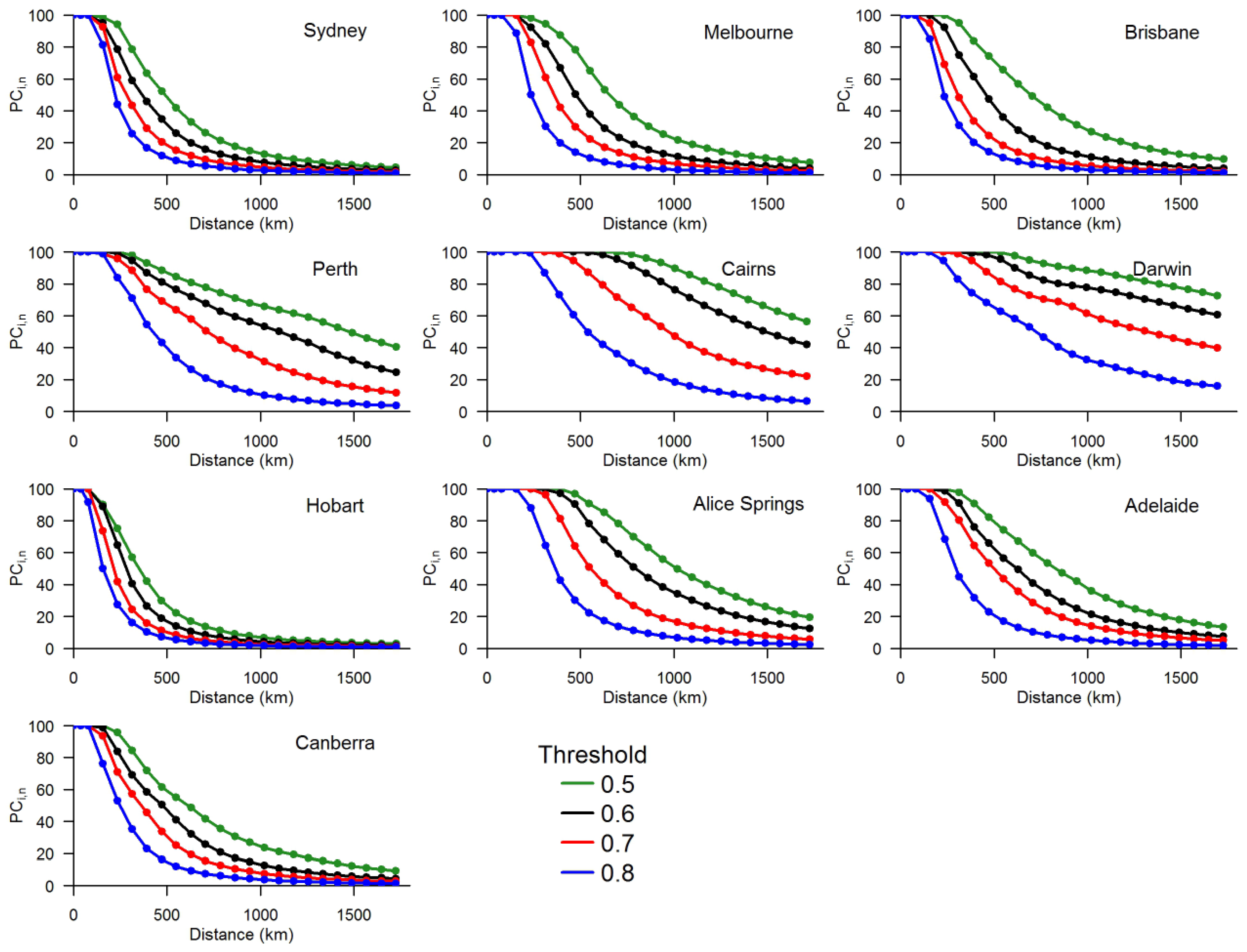
• Rainfall in Darwin and Cairns shows very significant correlations among grids for any threshold up to about 300 km or greater. Even in the most stringent case (T = 0.8), about 90–100% of grids have rainfall correlations exceeding the correlation threshold. It is relevant to note that these two cities have a tropical climate, with tropical savannah in Darwin and tropical rainforest (monsoonal) in Cairns.
• Rainfall in Hobart and Sydney shows particularly low correlations among grids for any of the threshold levels, with Hobart showing the worst results. In the most stringent case (T = 0.8), the distance up to which 90–100% of grids exceed the correlation threshold is only about 100 km. Even in the most relaxed case, i.e., “average” threshold of 0.5, 90–100% of grids exceed the threshold only up to about 250 km, especially for Hobart. It is relevant to note that these two cities have a temperate, no dry season climate, with a mild summer in Hobart and a hot summer in Sydney.
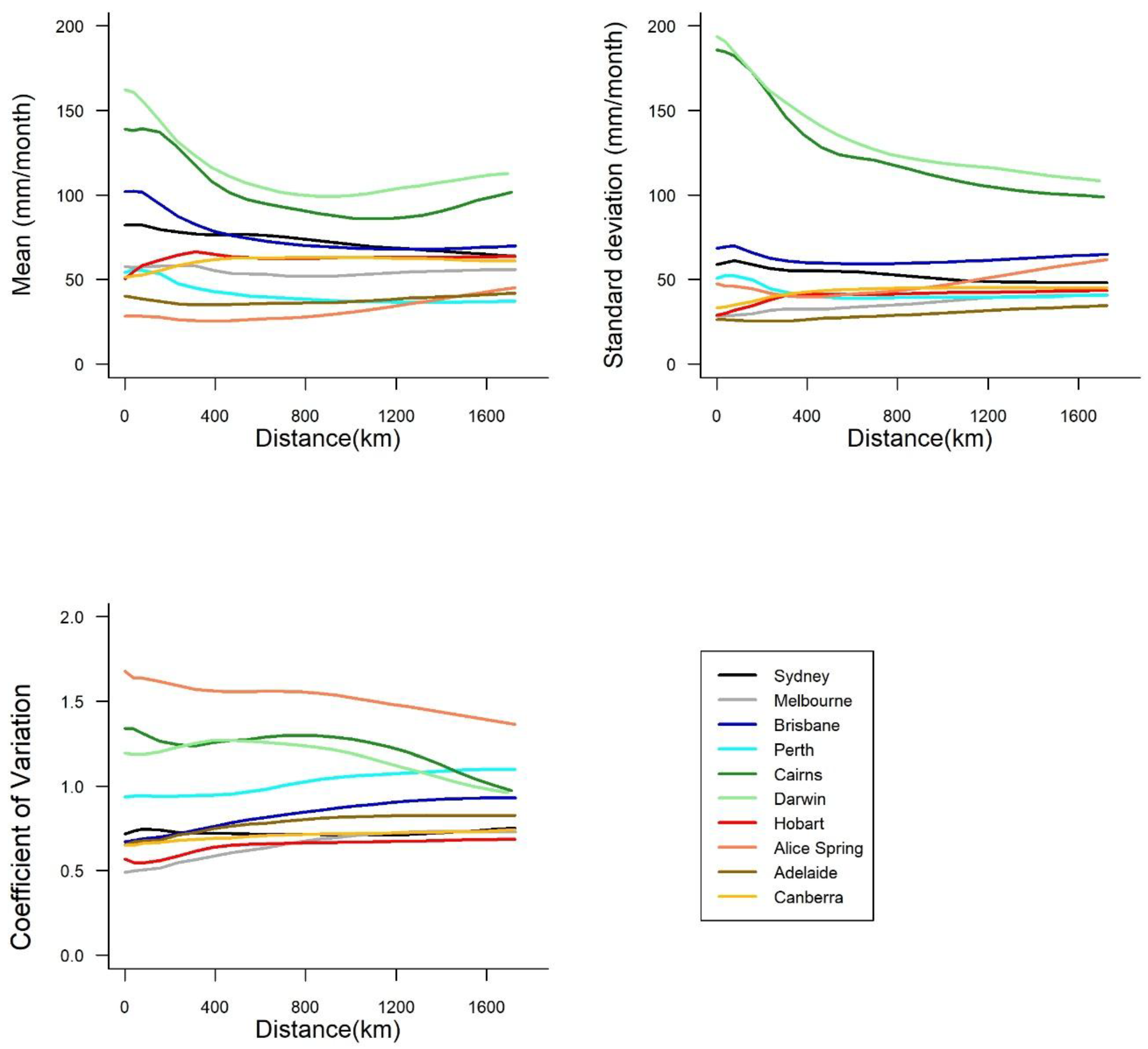
• Between Darwin and Cairns on one hand (tropical climate) and Hobart and Sydney on the other (temperate, no dry season climate), rainfall correlations among grids show a decreasing trend for, in order, Perth, Alice Springs, Adelaide, Canberra, Melbourne, and Brisbane, although some differences exist for different thresholds. These results also seem to suggest that spatial rainfall correlations among grids decrease from a temperate (no dry season) climate to a grassland (persistently dry) climate to a subtropical (distinctly dry summer) climate, with others in between. Nevertheless, there can certainly be exceptions to this interpretation. This is because, even if the climates in two cities are approximately similar, possible bias in spatial rainfall correlations may also occur due to many other factors that influence rainfall both within and surrounding the cities. On the other hand, rainfall statistical properties in two cities can be significantly different even when the cities have approximately similar climates. A comparison of the spatial rainfall correlation results in Figure 6 with the rainfall statistics (mean, standard deviation, and coefficient of variation—standard deviation/mean) in Figure 7 for the ten cities seems to suggest the possible inconsistencies and complications that may arise in interpreting the spatial rainfall correlation results and/or rainfall statistics; see, for instance, the results for Alice Springs and Adelaide. Therefore, proper care needs to be exercised in interpreting the spatial rainfall correlations and rainfall statistics, towards rainfall interpolation/extrapolation. We will examine these issues in more detail in a future study.

5. Study Implications and Further Research

The above spatial rainfall results for Australia and the ten major cities have important implications for a range of studies on rainfall and on water resources and the environment at large. At the most fundamental level, they are useful (1) to assess whether or not an(y) interpolation scheme(s) is necessary or effective for a given region; (2) to determine which interpolation scheme can be more effective for which region, and why; (3) to identify “critical” points or areas at which installing rain gauges will significantly help in rainfall estimation, including for interpolation; and (4) to “classify” regions in terms of spatial rainfall correlations, especially towards estimating rainfall in regions that have absolute scarcity of data or even no data.

For instance, considering all of Australia, rainfall dynamics in northern and northeastern Australia have far greater spatial correlations when compared to those in southern and southeastern Australia. This may imply that tropical climates generally have greater spatial rainfall correlations when compared to, for example, temperate, grassland, and desert climates, subject to other influencing factors (see below). This seems to suggest that rainfall interpolation schemes (if based on data available at a 0.25° × 0.25° resolution or greater) will not be particularly effective in southern and southeastern Australia when compared to in northern and northeastern regions. An important implication of this may be that rain gauges need to be installed much closer together in the former areas when compared to the latter in order to obtain more reliable rainfall estimates, including using interpolation schemes.

In addition to climate type (e.g., tropical, temperate, grassland, desert), several other factors drive rainfall dynamics and, hence, dictate spatial rainfall correlations. These include topography (especially elevation), wind (direction and velocity), and proximity to the coast, among others. Studying whether, how, and to what extent these factors influence rainfall dynamics and spatial variability has been an important area of research for many years now; see [8,42]. Although the present study does not delve into these factors, the results reveal the potential complications and inconsistencies in offering interpretations in one way or another. For instance, while it is known that coastal proximity plays a definite role in rainfall dynamics at a location, the differences (sometimes significant) in spatial correlations obtained for the coastal cities studied here (except Alice Springs and Canberra, all cities are along or just a few kilometers from the coast) reflect the difficulties in providing general interpretations on its role and specific details about its extent.

The results from the present study clearly highlight the need for a combined rainfall correlation-spatial scale-correlation threshold approach for studying rainfall spatial variability and interpolation more effectively and efficiently. The study addresses a very fundamental question on spatial rainfall correlations, i.e., to assess whether rainfall interpolation based on existing data (at other resolutions) will be effective before any interpolation scheme is employed. The Australia-wide analysis and the city-based analysis clearly bring out the general and specific benefits of the methodology presented here by providing useful information for the identification of “similar regions” or “clusters” of rainfall correlation (to help with studies on “ungauged” regions) and determination of the optimum (or effective) interpolation distance (to help with the assessment of rain gauge locations and density), among others. To this end, the results reported by complex networks-based studies for Australian rainfall [10,22,43], which provide useful information about the dominant rain gauge stations/regions, can also play an important role. How the present approach and the complex networks-based approach can supplement and complement each other remains to be seen. Investigations in this direction are currently underway, details of which will be reported elsewhere.

References

1. Thiessen, A.H. Precipitation averages for large areas. Mon. Weather Rev. 1911, 39, 1082–1084. [Google Scholar] [CrossRef]
2. Eagleson, P.S. Optimum density of rainfall networks. Water Resour. Res. 1967, 3, 1021–1033. [Google Scholar] [CrossRef]
3. Zawadzki, I.I. Statistical properties of precipitation patterns. J. Appl. Meteorol. 1973, 12, 459–472. [Google Scholar] [CrossRef]
4. Berndtsson, R. Temporal variability in spatial correlation of daily rainfall. Water Resour. Res. 1988, 24, 1511–1517. [Google Scholar] [CrossRef]
5. Krstanovic, P.F.; Singh, V.P. Evaluation of rainfall networks using entropy: I. Theoretical development. Water Resour. Manag. 1992, 6, 279–293. [Google Scholar] [CrossRef]
6. Krstanovic, P.F.; Singh, V.P. Evaluation of rainfall networks using entropy: II. Application. Water Resour. Manag. 1992, 6, 295–314. [Google Scholar] [CrossRef]
7. McCollum, J.R.; Krajewski, W.F. Uncertainty of monthly rainfall estimates from rain gauges in the global precipitation climatology project. Water Resour. Res. 1998, 34, 2647–2654. [Google Scholar] [CrossRef]
8. Garcia, M.; Peters-Lidard, C.D.; Goodrich, D.C. Spatial interpolation of precipitation in a dense gauge network for monsoon storm events in the southwestern united states. Water Resour. Res. 2008, 44, W05S13. [Google Scholar] [CrossRef]
9. Mishra, A.K.; Coulibaly, P. Hydrometric network evaluation for canadian watersheds. J. Hydrol. 2010, 380, 420–437. [Google Scholar] [CrossRef]
10. Sivakumar, B.; Woldemeskel, F.M. A network-based analysis of spatial rainfall connections. Environ. Model. Softw. 2015, 69, 55–62. [Google Scholar] [CrossRef]
11. Shi, H.; Li, T.; Wei, J.; Fu, W.; Wang, G. Spatial and temporal characteristics of precipitation over the three-river headwaters region during 1961–2014. J. Hydrol. Reg. Stud. 2016, 6, 52–65. [Google Scholar] [CrossRef]
12. Lakew, H.B.; Mogus, S.A.; Asfaw, D.H. Hydrological evaluation of satellite and reanalysis precipitation products in the Upper Blue Nile Basin: A case study of Gilgel Abbay. Hydrology 2017, 4, 39. [Google Scholar] [CrossRef]
13. Chen, A.; Chen, D.; Azorin-Molina, C. Assessing reliability of precipitation data over the Mekong River Basin: A comparison of ground-based, satellite, and reanalysis data sets. Int. J. Climatol. 2018, 38, 4314–4334. [Google Scholar] [CrossRef]
14. Wang, W.; Wang, D.; Singh, V.P.; Wang, Y.; Wu, J.; Wang, L.; Zou, X.; Liu, J.; Zou, Y.; He, R. Optimization of rainfall networks using information entropy and temporal variability analysis. J. Hydrol. 2018. [Google Scholar] [CrossRef]
15. Huffman, G.J.; Adler, R.F.; Rudolf, B.; Schneider, U.; Keehn, P.R. Global precipitation estimates based on a technique for combining satellite-based estimates, rain gauge analysis, and NWP model precipitation information. J. Clim. 1995, 8, 1284–1295. [Google Scholar] [CrossRef]
16. Li, M.; Shao, Q. An improved statistical approach to merge satellite rainfall estimates and raingauge data. J. Hydrol. 2010, 385, 51–64. [Google Scholar] [CrossRef]
17. Woldemeskel, F.M.; Sivakumar, B.; Sharma, A. Merging gauge and satellite rainfall with specification of associated uncertainty across australia. J. Hydrol. 2013, 499, 167–176. [Google Scholar] [CrossRef]
18. Shi, H.; Li, T.; Wei, J. Evaluation of the gridded CRU TS precipitation dataset with the point raingauge records over the Three-River Headwaters region. J. Hydrol. 2017, 548, 322–332. [Google Scholar] [CrossRef]
19. Sivakumar, B.; Sorooshian, S.; Gupta, H.V.; Gao, X. A chaotic approach to rainfall disaggregation. Water Resour. Res. 2001, 37, 61–72. [Google Scholar] [CrossRef]
20. Li, J.; Bárdossy, A.; Guenni, L.; Liu, M. A copula based observation network design approach. Environ. Model. Softw. 2011, 26, 1349–1357. [Google Scholar] [CrossRef]
21. Niu, J. Precipitation in the Pearl River basin, South China: Scaling, regional patterns, and influence of large-scale climate anomalies. Stoch. Environ. Res. Risk Assess. 2013, 27, 1253–1268. [Google Scholar] [CrossRef]
22. Jha, S.K.; Sivakumar, B. Complex networks for rainfall modeling: Spatial connections, temporal scale, and network size. J. Hydrol. 2017, 554, 482–489. [Google Scholar] [CrossRef]
23. Kummerow, C.; Simpson, J.; Thiele, O.; Barnes, W.; Chang, A.T.C.; Stocker, E.; Adler, R.F.; Hou, A.; Kakar, R.; Wentz, F.; et al. The status of Tropical Rainfall Measuring Mission (TRMM) after two years in orbit. J. Appl. Meteorol. 2000, 39, 1965–1982. [Google Scholar] [CrossRef]
24. Fleming, K.; Awange, J.L.; Kuhn, M.; Featherstone, W.E. Evaluating the TRMM 3B43 monthly precipitation product using gridded raingauge data over Australia. J. South. Hemisph. Earth Syst. Sci. 2011, 61, 171–184. [Google Scholar] [CrossRef]
25. Taschetto, A.S.; England, M.H. An analysis of late twentieth century trends in australian rainfall. Int. J. Clim. 2009, 29, 791–807. [Google Scholar] [CrossRef]
26. Stern, H.; De Hoedt, G.; Ernst, J. Objective classification of Australian climates. Aust. Meteorol. Mag. 2000, 49, 87–96. [Google Scholar]
27. Guo, D.; Westra, S.; Maier, R.H. Sensitivity of potential evapotranspiration to changes in climate variables for different Australian climate zones. Hydrol. Earth Syst. Sci. 2017, 21, 2107–2126. [Google Scholar] [CrossRef]
28. Jeffrey, S.J.; Carter, J.O.; Moodie, K.B.; Beswick, A.R. Using spatial interpolation to construct a comprehensive archive of Australian climate data. Environ. Model. Softw. 2001, 16, 309–330. [Google Scholar] [CrossRef]
29. Chiew, F.H.S.; Young, W.J.; Cai, W.; Teng, J. Current drought and future hydroclimate projections in southeast australia and implications for water resources management. Stoch. Environ. Res. Risk Assess. 2010, 25, 601–612. [Google Scholar] [CrossRef]
30. Chiew, F.H.S.; Potter, N.J.; Vaze, J.; Petheram, C.; Zhang, L.; Teng, J.; Post, D.A. Observed hydrologic non-stationarity in far south-eastern australia: Implications for modelling and prediction. Stoch. Environ. Res. Risk Assess. 2014, 28, 3–15. [Google Scholar] [CrossRef]
31. Sivakumar, B.; Woldemeskel, F.M.; Puente, C.E. Nonlinear analysis of rainfall variability in australia. Stoch. Environ. Res. Risk Assess. 2014, 28, 17–27. [Google Scholar] [CrossRef]
32. Chokngamwong, R.; Chiu, L.S. Thailand daily rainfall and comparison with trmm products. J. Hydrometeorol. 2008, 9, 256–266. [Google Scholar] [CrossRef]
33. Chiu, L.S.; Liu, Z.; Vongsaard, J.; Morain, S.; Budge, A.; Neville, P.; Bales, C. Comparison of trmm and water district rain rates over new mexico. Adv. Atmospheric Sci. 2006, 23, 1–13. [Google Scholar] [CrossRef]
34. Hughes, D.A. Comparison of satellite rainfall data with observations from gauging station networks. J. Hydrol. 2006, 327, 399–410. [Google Scholar] [CrossRef]
35. AghaKouchak, A.; Nasrollahi, N.; Habib, E. Accounting for uncertainties of the TRMM satellite estimates. Remote Sens. 2009, 1, 606–619. [Google Scholar] [CrossRef]
36. Guofeng, Z.; Dahe, Q.; Yuanfeng, L.; Fenli, C.; Pengfei, H.; Dongdong, C.; Kai, W. Accuracy of trmm precipitation data in the southwest monsoon region of china. Theor. Appl. Clim. 2016. [Google Scholar] [CrossRef]
37. Grimes, D.I.; Pardo-Igúzquiza, E.; Bonifacio, R. Optimal areal rainfall estimation using raingauges and satellite data. J. Hydrol. 1999, 222, 93–108. [Google Scholar] [CrossRef]
38. Collischonn, B.; Collischonn, W.; Tucci, C.E.M. Daily hydrological modeling in the amazon basin using trmm rainfall estimates. J. Hydrol. 2008, 360, 207–216. [Google Scholar] [CrossRef]
39. Su, F.; Hong, Y.; Lettenmaier, D.P. Evaluation of trmm multisatellite precipitation analysis (tmpa) and its utility in hydrologic prediction in the La Plata basin. J. Hydrometeorol. 2008, 9, 622–640. [Google Scholar] [CrossRef]
40. Yong, B.; Hong, Y.; Ren, L.-L.; Gourley, J.J.; Huffman, G.J.; Chen, X.; Wang, W.; Khan, S.I. Assessment of evolving trmm-based multisatellite real-time precipitation estimation methods and their impacts on hydrologic prediction in a high latitude basin. J. Geophys. Res. Atmos. 2012, 117, D09108. [Google Scholar] [CrossRef]
41. Naufan, I.; Sivakumar, B.; Woldemeskel, F.M.; Raghavan, S.V.; Wu, M.T.; Liong, S.-Y. Spatial connections in regional climate model rainfall outputs at different temporal scales: Application of network theory. J. Hydrol. 2018, 556, 1232–1243. [Google Scholar] [CrossRef]
42. Kurtzman, D.; Navon, S.; Morin, E. Improving interpolation of daily precipitation for hydrologic modelling: Spatial patterns of preferred interpolators. Hydrol. Process. 2009, 23, 3281–3291. [Google Scholar] [CrossRef]
43. Jha, S.K.; Zhao, H.; Woldemeskel, F.M.; Sivakumar, B. Network theory and spatial rainfall connections: An interpretation. J. Hydrol. 2015, 527, 13–19. [Google Scholar] [CrossRef]
Figure 1. Schematic representation of the spatial rainfall estimation problem. Grid i is the base grid and grids j are the neighborhood grids in a given box size n (j = 1, 2, 3, …, N − 1, where N is the total number of grids within a box size).
Hydrology 06 00011 g001
Figure 2. Map of Australia and locations of ten cities considered for spatial rainfall correlation analysis. The climate division of Australia is according to Köppen climate classification and its modification (after [27]).
Hydrology 06 00011 g002
Figure 3. Spatial rainfall correlations for 0.25° × 0.25° grids across Australia for threshold (T) = 0.6. The results correspond to eight different box sizes (n = 1, 6, 12, 18, 24, 30, 36, and 42) and indicate the percentage of grids exceeding (PCi,n) the threshold value.
Hydrology 06 00011 g003
Figure 4. Same as Figure 3, but for threshold (T) = 0.8.
Hydrology 06 00011 g004
Figure 5. Spatial rainfall correlations for ten cities in Australia. Each plot presents PCi,n for 23 box sizes for four threshold levels (T = 0.5, 0.6, 0.7, and 0.8) for the respective city.
Hydrology 06 00011 g005
Figure 6. Spatial rainfall correlations for ten cities in Australia. Each plot presents PCi,n for 23 box sizes for all cities with T = 0.5 (top left), T = 0.6 (top right), T = 0.7 (bottom left), and T = 0.8 (bottom right).
Hydrology 06 00011 g006
Figure 7. Rainfall statistics vs. distance for ten cities in Australia: mean (top left), standard deviation (top right), and coefficient of variation (bottom).
Hydrology 06 00011 g007