Mitigating Spatial Discontinuity of Multi-Radar QPE Based on GPM/KuPR

Abstract

Reflectivity factor bias caused by radar calibration errors would influence the accuracy of Quantitative Precipitation Estimations (QPE), and further result in spatial discontinuity in Multiple Ground Radars QPE (MGR-QPE) products. Due to sampling differences and random errors, the associated discontinuity cannot be thoroughly solved by the single-radar calibration method. Thus, a multiple-radar synchronous calibration approach was proposed to mitigate the spatial discontinuity of MGR-QPE. Firstly, spatial discontinuity was solved by the intercalibration of adjacent ground radars, and then calibration errors were reduced by referring to the Ku-Band Precipitation Radar (KuPR) carried by the Global Precipitation Measurement (GPM) Core Observatory as a standard reference. Finally, Mosaic Reflectivity and MGR-QPE products with spatial continuity were obtained. Using three S-band operational radars covering the lower reaches of the Yangtze River in China, this method was evaluated under four representative precipitation events. The result showed that: (1) the spatial continuity of reflectivity factor and precipitation estimation fields was significantly improved after bias correction, and the reflectivity differences between adjacent radars were reduced by 78% and 82%, respectively; (2) the MGR-QPE data were closer to gauge observations with the normalized absolute error reducing by 0.05 to 0.12.

1. Introduction

Weather radar is able to retrieve rainfall based on the statistical relationship between the reflectivity factor (Z) and rain rate (R), namely the Z–R relation [1]. Quantitative Precipitation Estimation (QPE) is affected by many factors, e.g., precipitation Drop Size Distribution (DSD), ground clutter contamination, sampling error and beam overshooting [2,3], where radar calibration error is an essential factor [4], and it covers miscalibrations of transmission power, waveguide loss, antenna gain and receiver gain. Radar equation suggests that calibration error would result in a reflectivity factor bias that changes the intrinsic precipitation estimation relation. Rosenfeld and Ulbrich [5] showed more than 200 Z–R relationships to be reported, which were too many to be totally explained by DSD variability, maybe owing to calibration errors [4].

Given the limited coverage of single ground radar, Multiple Ground Radars QPE (MGR-QPE) is more feasible for large-scale precipitation product. However, Seo et al. [6] noted for the first time that calibration error would result in the spatial discontinuity of MGR-QPE, especially in overlapping areas of ground radars, which severely reduce the QPE accuracy and also affect hydrological predictions. Brandes et al. [7] compared the precipitation estimations between two collocated radars in the United States and found the precipitation data recorded by NCAR S-Pol (National Center for Atmospheric Research’s S-band, dual-polarization radar) were smaller than that recorded by WSR-88D (Weather Surveillance Radar, 1988, Doppler) and by rain gauges. Smith et al. [8] found the QPE data in radar overlapping areas were significantly different between two neighboring radars, Tulsa and Twin Lakes, in the United States due to the interference of calibration errors, and the mean rainfall of Tulsa was 30% higher than that of Twin Lakes. Gourley et al. [9] indicated that a discrepancy of 2–3 dB between reflectivities measured by adjacent WSR-88D radars was quite common, and that the inconsistency between radars would lead to spatial discontinuity for MGR-QPE. You et al. [10] analyzed several ground radars in South Korea and found the largest difference of reflectivity was up to 12 dB. Xiao and Liu [11] reported that the difference of S-band operational radars in South China was around 3 dB.

Although there are many radar calibration methods, calibration errors can be hardly reduced within 1 dB [12]. Hardware calibration with instruments is difficult to obtain full-path errors including receiver, transmitter, antenna and waveguides. Standard floating metal ball approach is not easy to operate and cannot be used frequently [13]. The methods referring to rain gauges or disdrometers are more feasible for qualitative assessment, but are not acceptable for quantitative calibration, due to spatiotemporal variability and different observations [14]. Although intercalibration between adjacent ground radars is reliable, it is difficult to decide which radar is more accurate. More recently, the wide-covering and well-calibrated Tropical Rainfall Measuring Mission/Precipitation Radar (TRMM/PR) became more popular to the public [15,16,17] and was used as a reference to estimate the calibration errors of ground radars [18,19,20]. Anagnostou et al. [21] showed that the calibration errors of WSR-88D radars were +2 to −7 dB compared with the PR data. Wang and Wolff [22] statistically analyzed the calibration errors of four primary TRMM ground validation radars.

Reducing calibration errors and mitigating spatial discontinuity are equally important for MGR-QPE. The TRMM/PR-based single ground radar (GR) calibration method is able to reduce the calibration errors. However, it is difficult to address the spatial discontinuity of multiple radars products because of the differences in hardware parameters, sampling volumes and random errors between GR and TRMM/PR. As each of the GR is calibrated separately, spatial discontinuity may still exist. Although intercalibration of GRs is reliable to solve the spatial discontinuity, it is difficult to determine which GR is more accurate and further eliminate absolute calibration errors. Therefore, in this study, these two ideas were naturally combined, and a new approach is proposed with the involvement of the Global Precipitation Measurement/Ku-Band Precipitation Radar (GPM/KuPR) to obtain the MGR-QPE products with spatial continuity and higher accuracy.

This paper is organized as follows. Section 2 introduces the data of GRs, KuPR, rain gauges, and a disdrometer. Section 3 presents the hypothesis conditions and the proposed approach. In Section 4, the new method is evaluated using four representative precipitation events. Finally, the advantages and limitations of the proposed method are summarized and discussed in Section 5.

2. Data Sources

The downstream of the Yangtze River is a major residential and economic region of China, but is frequently influenced by severe weather, such as mei-yu heavy rain, typhoons and local strong convective storms. Thus, MGR-QPE is an important radar product for flood prediction and disaster weather nowcasting in this region.

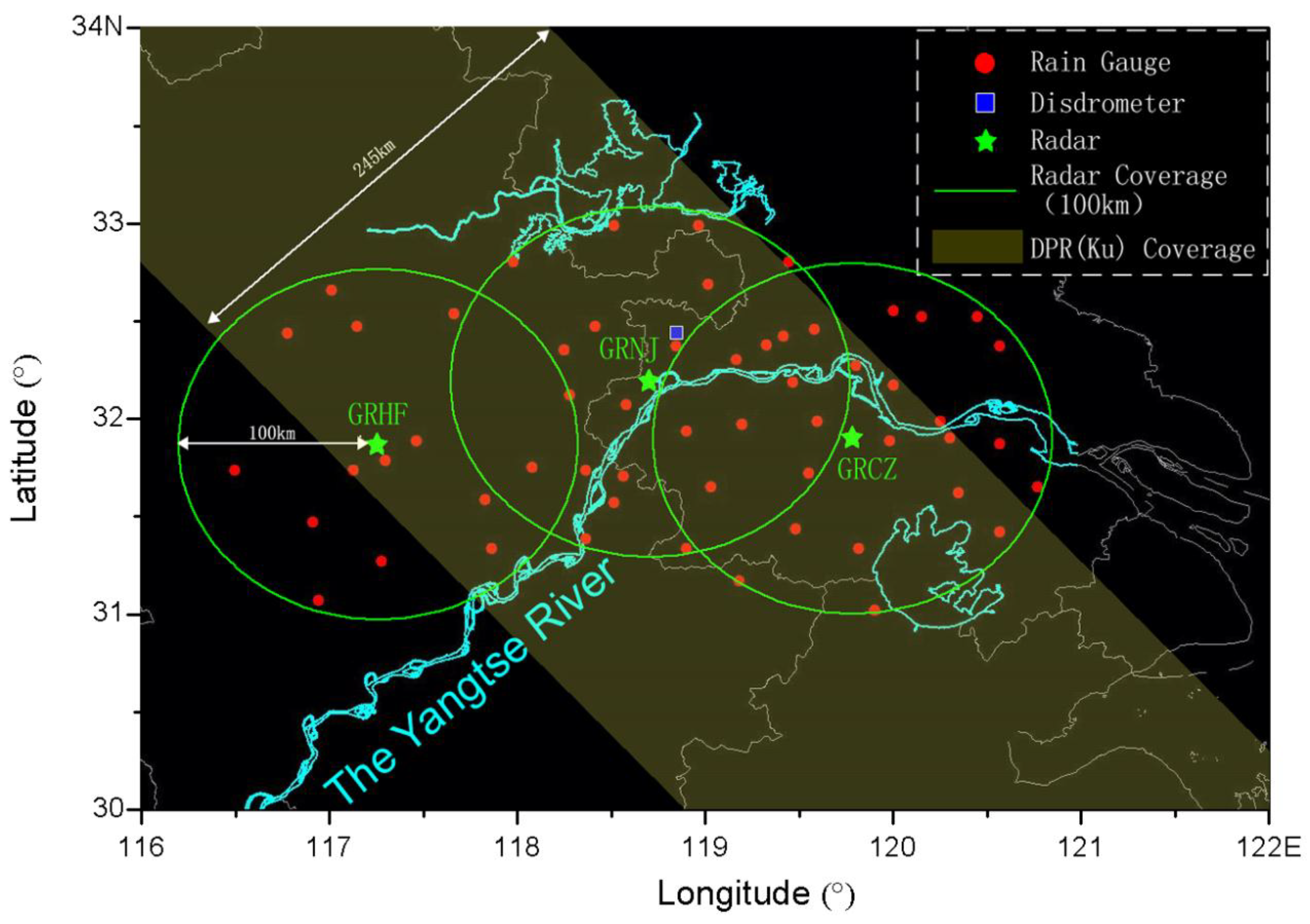
2.1. Ground Radar Data

Three S-band single polarization GRs covering the lower reaches of the Yangtze River were selected—GRHF (Ground Radar at Hefei, Anhui Province), GRNJ (Ground Radar at Nanjing, Jiangsu Province) and GRCZ (Ground Radar at Changzhou, Jiangsu Province). The locations and 100 km radius coverages of the three radars are shown in Figure 1. These radars were all CINRAD-SA (China New-generation Weather Radar S-band A-type), similar to previous single polarization WSR-88D in the United States (wavelength: 10 cm; elliptic paraboloid antenna diameter: 8.5 m; resolution: 1° by 1 km). All GRs operated volume scans of nine elevation angles from 0.5° to 19.5°, and the scan time was 5–6 min [23]. The surveillance radius was 460 km, and the effective radius in precipitation estimation was 100 km (green circle in Figure 1). The GR volume scan raw data, consisting of nine elevation angles, were used in this study. The GR data were processed by quality control using the operational Severe Weather Nowcast System (SWAN) [24] developed by the China Meteorological Administration, including noise filtering and ground clutter suppression. The ground clutter blockage was marked by manual recognition and modification.

2.2. Rain Measurement Data

There was one OTT Parsivel² disdrometer (blue rectangle in Figure 1) and 56 national operational rain gauges in the coverages of the three GRs. The OTT Parsivel² disdrometer was a modification of OTT Parsivel [25] and could measure rain DSD and fall velocities for particle sizes from 0.3 to 20 mm. On the conditions that precipitation rate > 0.1 mm/h and the total number of particles > 10, the noisy light rain data were removed from 1-min DSD. The selected DSD data were used to evaluate the reflectivities of KuPR and calculate the difference in scattering between the Ku-band and S-band (Section 3). The data from the operational rain gauges were used to evaluate MGR-QPE (Section 4). The measured rain data were processed by quality control, including: (1) national climatological threshold value check; (2) regional climatological threshold value check; (3) temporal consistency check; and (4) spatial consistency check [26].

2.3. GPM/KuPR Data

The GPM Core Observatory was launched on 28 February 2014 to take over TRMM as the core satellite for global precipitation measurement, and was jointly maintained by NASA (the National Aeronautics and Space Administration, Washington, DC, USA) of the United States and JAXA (The Japan Aerospace Exploration Agency, Tokyo, Japan) of Japan. At a flying height of 407 km GPM carried a dual-frequency PR with phase array antenna, namely the 13.6 GHz KuPR and the 35.5 GHz KaPR (Ka-Band Precipitation Radar). Compared with the single-frequency precipitation radar of TRMM, GPM/DPR had stronger weak-precipitation detecting ability, finer vertical resolution and broader spatial coverage (68° N/S) [27]. The swath of KuPR was 245 km, the horizontal resolution was 5 km, vertical resolution was 125 m (resampled) and the detectable minimum was ~18 dBZ. The GPM/KuPR Level-2 data provided by the Precipitation Processing System of Goddard Space Flight Center (https://pps.gsfc.nasa.gov/) were used to calibrate three S-Band GRs in this research (Section 3 and Section 4), including the 3D corrected reflectivities, precipitation types and bright band information.

3. Methodology

The single-GR calibration method based on satellite-borne precipitation radar can only calibrate one GR at a time, and does not consider the spatial continuity of multiple radars products, such as the Available Best Comparable Dataset method (ABCD) [18]. For this reason, a GPM/KuPR-based multiple-GR calibration method was put forward and named M-ABCD.

3.1. Hypotheses of M-ABCD

Similar to single-GR’s ABCD method, the M-ABCD method also has two main assumptions. The first assumption is that the corrected reflectivity factor of KuPR in GPM Level-2 product is relatively accurate, or the calibration errors of KuPR are far smaller than those of GRs. One task of GPM is to provide a standard reference for global precipitation estimation, so as to improve the effect of such estimation [27]. Both KuPR and TRMM/PR have undergone scientific internal and external calibrations, and thus as expected had very small calibration errors. Additionally, the Level-2 data performed several kinds of quality control, including beamfilling corrections, clutter rejection near the surface, and attenuation correction. In particular, since the attenuation of KuPR was corrected using double-frequency algorithms [28,29], KuPR outperformed the hybrid of a Hitschfeld–Bordan and a Surface Reference Technique of TRMM [30]. Iguchi et al. [31] found the corrected data of KuPR were accurate, and the precipitation estimations of KuPR were closer to measurements of rain gauges than TRMM/PR.

To deeply understand the accuracy of KuPR in China, we adopted the DSD spectral measurements of the disdrometer (Figure 1) to simply evaluate the reflectivity factor of KuPR. Firstly, the KuPR and disdrometer were matched in space and time to find the available precipitation events. Due to the complex temporal and spatial changes of convective precipitation, here we only select stratiform data for analysis. Specifically, the selected precipitation data met the standard deviation of the DSD rainfall rate <1.5 mm/h in 10 min [32] and stratiform type in GPM precipitation classification. Afterwards, the DSD data with simple quality control (introduced in Section 2) were accumulated to 10 min by summing the number of particles in each bin and fitted by gamma distribution to form the three fitting parameters ($\mu$, $\mathsf{\Lambda }$, $N_0$) [33]. The 10-min accumulation and gamma fitting were aimed to reduce the random observational errors of DSD, especially for the data from the first two low signal-to-noise ratio channels. From the DSD measured between April and October 2016, we found 17 qualified stratiform precipitation events paired with KuPR, and used T-Matrix [34,35] to simulate the horizontal reflectivity factor Z of 13.6 GHz, and compared with the average Z values of KuPR at heights of 0.5–1.5 km (this height avoided contamination from ground clutters and bright band). In the T-Matrix simulation, the raindrop shape was described using the Beard and Chuang [36] relation, the zenith angle of the incident beam was 0° and the temperature was set at 10 °C. It was also assumed that the drops are canted with the mean canting angle equal to zero and 10° standard deviation of the Gaussian distribution of the canting angle. More details about DSD parameterization, raindrop shape, and T-Matrix simulation can be found in Kalogiros et al. [37]. In Figure 2a, the KuPR observations and the DSD simulation are very consistent, with correlation coefficient > 0.93, and the mean values are all very close. It can be generally expected that the observed data of GPM/KuPR meet the first hypothesis. The high correlation coefficient in Figure 2a was attributed to the following two reasons: (1) the accumulation of DSD in time (10 min) and average of KuPR in space (horizontal 5 km, vertical 1 km, 9 points) were able to reduce observational errors; (2) stable stratiform rainfall was more favorable for decreasing the sampling volumes and time–space differences between DSD and KuPR. However, some inconsistency still exists. When KuPR is less than 22 dBZ, KuPR reflectivity is slightly greater than DSD simulation, which may be related to the low signal-to-noise ratio of KuPR or simulated errors of the T-Matrix (Figure 2b).

The second assumption of M-ABCD was that GR and GPM/KuPR were comparable. On one hand, GR and KuPR had the same observational principles. Many studies suggested GR and TRMM/PR were comparable (Section 1). As the successor of TRMM/PR, GPM/KuPR had all the same parameters as TRMM/PR, except for the visiting frequency and vertical resolution [38]. Thus, it can be anticipated that GR and KuPR are also comparable. On the other hand however, the scan modes and parameters were largely different between GR and KuPR, indicating the second hypothesis is not fully met. Therefore, the KuPR data should be corrected and filtered prior to comparison with GR.

GR and KuPR were mainly different in two aspects: Firstly, the scattering difference between the S-band and Ku-band was also the difference between the Mie scattering and Rayleigh scattering. In the previous TRMM/PR-based single-GR correction method, the relation from Liao and Meneghini [39] was used to correct the scattering difference. This relation was derived from the Marshall–Palmer rain DSD and Gunn–Marshall snow-size distribution according to the frequency of TRMM/PR, as shown by the Liao(Rain) and Liao(Snow) in Figure 3. Since the frequencies of KuPR (13.6 GHz) and PR (13.8 GHz) were slightly different, the radar frequency correction relation should also be adjusted slightly. The rain DSD data in 04–10, 2016 were used here, and T-Matrix was used to calculate the reflectivity at 13.6 and 3.0 GHz, as shown on the DSD (Rain) curve in Figure 3. The DSD data and the T-Matrix parameters were the same as in Section 3.1. The DSD(Rain) curve in Figure 3 shows that the Ku-band reflectivity was gradually larger than the S-band reflectivity, which was due to the Mie scattering in Ku-band. Moreover, the DSD simulated reflectivity was concentrated near the fitting curve, indicating that the scattering at Ku-band was definitely correlated with that at S-band. Therefore, the Ku-band data could be corrected using the DSD(Rain) curve for direct comparison with the S-band.

Another difference was the sampling volumes between KuPR and GR. The sampling volume of GR was 1 km × 1° × 1° and changed with distance, while the sampling volume of KuPR was 5 × 5 × 0.125 km³. KuPR and GR, when observing the uniform stratiform precipitation, would return consistent values. However, the differences would be incremented when they observed convective precipitation. The radar equation suggested that the calibration error $\Delta Z$ was independent of the precipitation type. Thus, $\Delta Z$ could be estimated by only using stratiform precipitation to reduce uncertainty. GPM used the measured dual-frequency ratio method to divide echoes into stratiform, convective and other type precipitation [38], which showed this classification was reasonable [40]. Thus, the stratiform data could be selected according to the GPM precipitation classification to reduce the difference of sampling volumes.

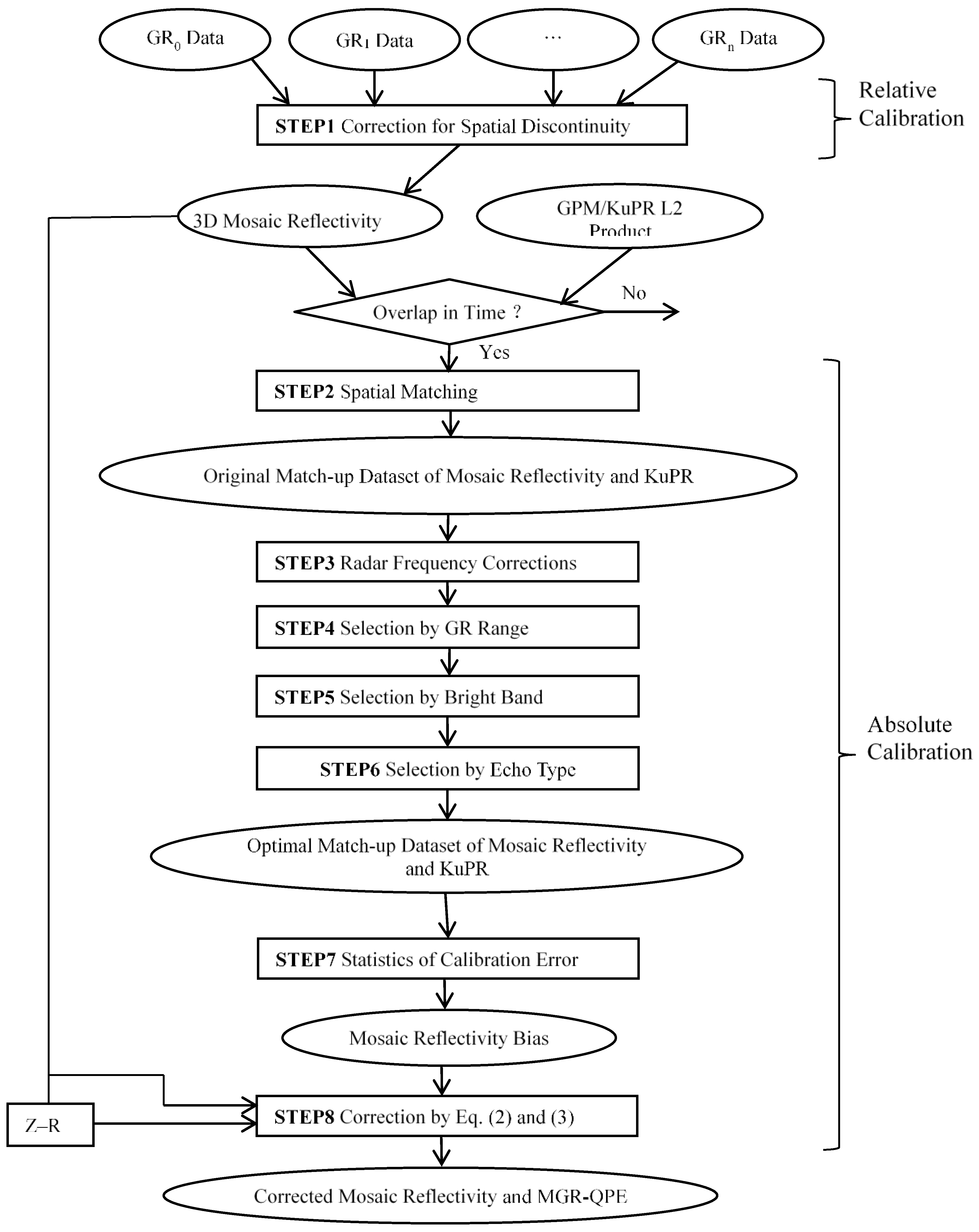
3.2. Details of M-ABCD Method

The flowchart of the proposed method is shown in Figure 4. M-ABCD consisted of eight steps, and its input data were the volume scan raw data of GRs and the Level-2 product of GPM/KuPR, and its output data were the corrected Mosaic Reflectivity. Logically, M-ABCD can be regarded to consist of two parts: relative calibration (STEP1) and absolute calibration (STEP2–STEP8). Each step will subsequently be elaborated.

STEP1 (Figure 4) was relative calibration that corrects the spatial discontinuity of GRs. Firstly, a GR was randomly selected as GR₀ and make the observed data of other GRs consistent with GR₀, namely had the same Z bias as GR₀. Generally, the radar centered in the study area was regarded as GR₀, which avoided the intercalibration error propagation. For instance, we selected the GRNJ centered in Figure 1 as GR₀. If GRCZ was selected as GR₀, we should use GRCZ to correct GRNJ and then use GRNJ to correct GRHF, which may lead to error propagation. The intercalibration adopted Equidistance Line Method that compared the mean reflectivities along the line that was equidistant between two adjacent GRs. On the equidistance line, the sampling volumes of two radars were the same, which may minimize the errors of comparison. To avoid effects from ground clutter and low signal-to-noise ratio, we only compared the reflectivities at more than 20 dBZ and vertical height >1.0 km. More details and discussion about relative calibration can be found in Seo et al. [41]. After that, the reflectivities of all GRs were mapped to 3D meshes of 1 × 1 × 0.5 km³ to form a Mosaic Reflectivity. In this study, the nearest-neighbor interpolation approach was used to process the overlapping areas, which highlighted the spatial discontinuity. Common interpolation methods, such as Cressman’s method [42], would smooth out the discontinuity and made discontinuity artificially disappear. After STEP1, the Mosaic Reflectivity was spatially continuous, but had a calibration error $\Delta Z$ (reflectivity bias), which was equal to the calibration error of GR₀.

STEP2–STEP8 in Figure 4 was absolute calibration that $\Delta Z$ of Mosaic Reflectivity was found using GPM/KuPR as the standard reference. Since comparison between GR and KuPR was somewhat uncertain (discussed in Section 3.1), here a stepwise selection method was developed, and the optimal match-up dataset was extracted from the Mosaic Reflectivity and KuPR. In STEP2, Spatial Matching, the commonly-used methods to match satellite and GR data include Sampling-Volume-Matching methods [43,44] and Grid-Matching methods [19,21,45]. Sampling-Volume-Matching aims to average the data according to the sampling volumes of GR and KuPR, forming match-up data. Grid-Matching aims to interpolate the GR and KuPR data into the same grid, forming match-up data. Sampling-Volume-Matching considers the differences in sampling volumes, but the number of samples acquired is relatively small. Grid-Matching does not consider the differences in sampling volumes, but returns more samples. Since M-ABCD requires a large size of paired samples for selecting, we adopted Grid-Matching method. The observed data of KuPR were mapped to the 3D Mosaic Reflectivity meshes, forming the original match-up dataset of Mosaic Reflectivity and KuPR. The matched Mosaic Reflectivity and KuPR were temporally close (≤3 min) and overlapped spatially (>1000 km²). STEP3 (radar frequency correction) of M-ABCD was to transform the rain reflectivity of KuPR to the S-band based on the DSD (Rain) relation shown in Figure 3. The reflectivity of KuPR (Ku Band) was adjusted to the frequency of GR (S Band), which reduced the observational difference due to different frequencies. In STEP4, Selection by GR Range, the paired data at a distance of 30–100 km from radar were extracted, and other data were excluded, so as to reduce the impacts of the ground clutters close to GRs and of the distant beam broadening. In STEP5, Selection by Bright Band, we selected the below-bright-band paired data and excluded the in-bright-band and above-bright-band data, according to the height and thickness of bright band provided by the GPM Level-2 products. The below-bright-band liquid raindrop data were selected because GR was highly correlated with the attenuation-corrected KuPR observed data and were far better than the in-bright-band or above-bright-band data [18,46]. In STEP6, Selection by Echo Type, according to the rain types provided by GPM Level-2 products, the data of convective precipitation (including other types of precipitation) were removed, and only stratiform precipitation was reserved. The stratiform precipitation and convective precipitation have the same $\Delta Z$ because the calibration error is independent of precipitation type. The exclusion of convective data can result in more reliable $\Delta Z$. After that, the resulting dataset was exactly the optimal match-up dataset in M-ABCD. In STEP7, Statistics of Calibration Error, the difference between the optimal matched Mosaic Reflectivity and KuPR, $X=\{x_i|x_i=Z_{M{R}_i}-Z_{KuP{R}_i}\}$, was used as a random variable, which obeyed Gaussian distribution, and the probability density function was $\mathrm{f}(X)$; then the expected value of $X$ was the calibration error $\Delta Z$ of Mosaic Reflectivity:

$$\Delta Z=E(X)={\displaystyle \int x_i\mathrm{f}(x_i)}$$

(1)

Relations among the corrected reflectivity factor $Z_c$ (dBZ), measured value $Z_m$ (dBZ) and calibration error $\Delta Z$ (dB) are shown as follows:

$$Z_c=Z_m+\Delta Z$$

(2)

The relationship between the corrected precipitation rate $R_c$ ($\mathrm{mm}\cdot {\mathrm{h}}^{-1}$) and the estimated precipitation rate $R_m$ ($\mathrm{mm}\cdot {\mathrm{h}}^{-1}$) from measured reflectivity can be expressed as follows:

$$R_c=R_m\times {10}^{\frac{\Delta Z}{10b}}$$

(3)

where $b$ was the Z–R coefficient. Finally, in STEP8, $Z_m$ was corrected to $Z_c$ using Equation (2) and $R_m$ was adjusted to $R_C$ using Equation (3). There were two practical ways to correct MGR-QPE. The first way was to apply the Z–R relationship to the raw Mosaic Reflectivity (outputted from STEP1) to obtain raw MGR-QPE, and then to correct MGR-QPE using Equation (3). The second way was to correct Mosaic Reflectivity using Equation (2) and then to retrieve precipitation using the Z–R relationship.

Essentially, M-ABCD includes two parts: relative correction of GRs (STEP1 in Figure 4) and absolute correction based on KuPR (STEP2–STEP8 in Figure 4). To respond the hypothesis in Section 3.1, we designed STEP3–STEP6 in M-ABCD for stepwise selection and correction, which eliminated the observational differences between GR and KuPR. STEP3 was able to correct the scattering differences at different frequencies. In STEP4, the GR data at 30–100 km were selected, which avoided the effects from ground clutters close to GR and from distant beam broadening. In STEP5, the liquid raindrop data below the bright band were selected. In STEP6, the stratiform data were selected, and the convective data with complex DSDs and difficulty in Ku-band attenuation correction were excluded, which reduced the uncertainty due to the differences in sampling volumes between KuPR and GR. It should be noted that STEP4–STEP6 of M-ABCD were three selection processes and their sequence could be changed. Moreover, the optimal match-up dataset from STEP6 was not really “optimal”, but was only relative to the original match-up dataset from STEP2 and its uncertainty was smaller.

4. Results

In order to investigate the performance of the M-ABCD approach, four typical precipitation events in the year of 2016 were selected: a light rainfall event on 9 May 2016, the Mei-yu rainband on 2 July 2016, the Typhoon Meranti rainband on 15 September 2016 and the frontal heavy rain event on 29 September 2016. For these events, rainfall areas were very large, and KuPR overlapped with the three GRs in Figure 1, which are favorable for the assessment below.

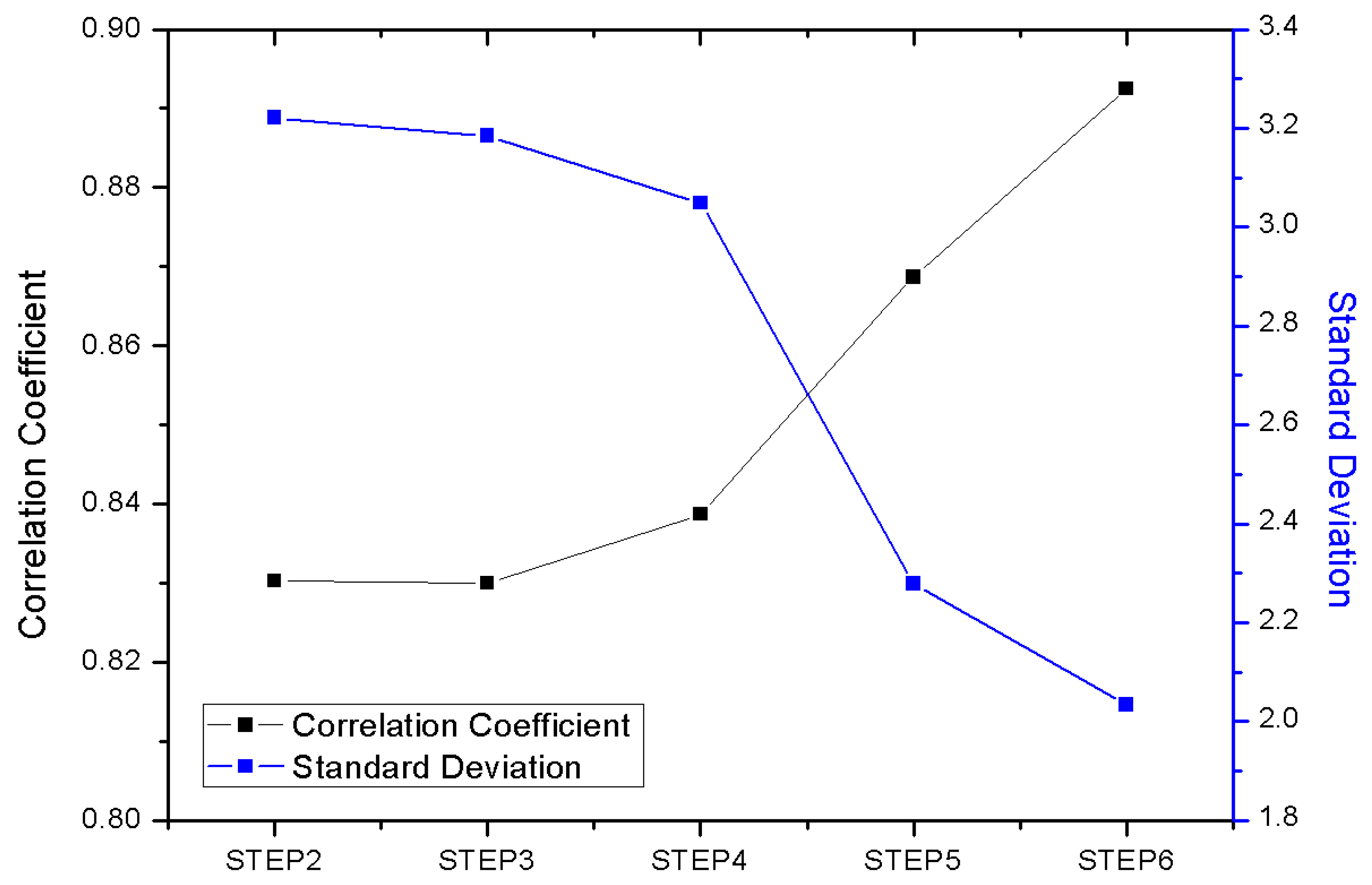
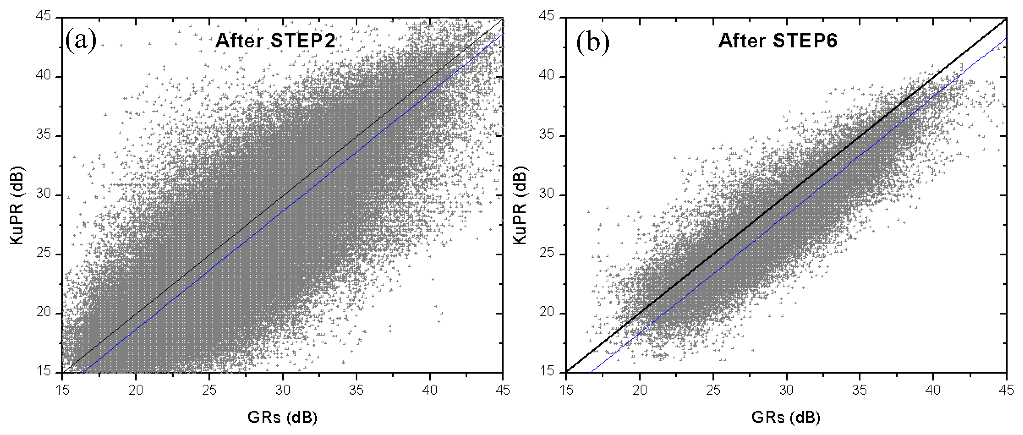
4.1. Effectiveness of STEP3–STEP6

In Figure 4, STEP1 and STEP2 of M-ABCD were very mature radar data processing techniques, and STEP7 and STEP8 were also very normal statistical and correction methods, which were all not discussed here. STEP3–STEP6 (Figure 4) were the key steps and decided the reliability of the results. To check the effectiveness of STEP3–STEP6, we selected the data on 29 September 2016 and analyzed the changes of the matched dataset after each step by using the correlation coefficient ${\rho }_{GK}$ between Mosaic Reflectivity and KuPR, the standard deviation ${\sigma }_{GK}$ of reflectivity factor difference. Larger values of ${\rho }_{GK}$ or ${\sigma }_{GK}$ indicate that the dataset was better, and smaller values indicate that the dataset was worse. In Figure 5, from the original matched data (STEP2) to the optimal matched data (STEP6), ${\rho }_{GK}$ gradually increased from 0.82 to 0.89, whereas ${\sigma }_{GK}$ gradually decreased by 37.5%. These changes in STEP3–STEP6 were effective, and after each selection step the match-up dataset gradually became better. Figure 6a,b show the original match-up dataset from STEP2 and the optimal match-up dataset from STEP6, respectively. Significantly, the points in Figure 6a were very scattered, indicating the presence of abundant abnormal data. After STEP3–STEP6, the points in Figure 6b became very concentrated, and the abnormal data were largely eliminated, so as to clearly show the linear relation between Mosaic Reflectivity and KuPR. The intercept of the blue fitted line was calibration error $\Delta Z$.

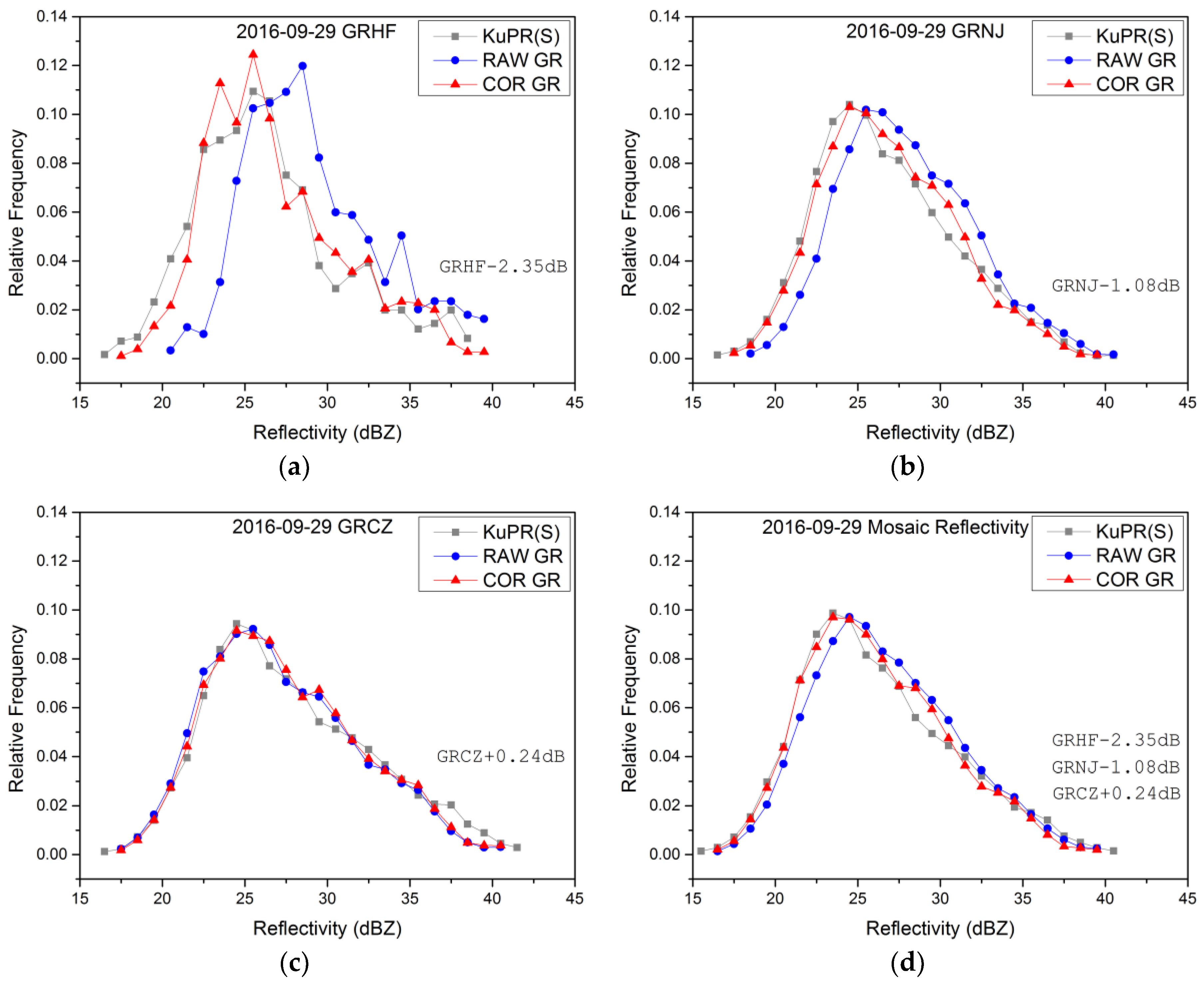
4.2. Corrected Reflectivity Distribution

In M-ABCD, the bias-correction method was used to adjust reflectivity (Equation 2). To clarify the difference between the raw and corrected reflectivities, we statistically analyzed the relative frequency of KuPR (after Radar Frequency Correction from Ku-Band to S-Band), raw GR and corrected GR reflectivity at the interval of 1 dB (Figure 7). When the calibration error $\Delta Z$ was smaller/larger than 0, the Probability Mass Function (PMF) of single-GR corrected reflectivity would preserve the original shape, and then shifted leftwards/rightwards as a whole to the PMF of KuPR. Since the $\Delta Z$ of GRHF (Figure 7a) and GRNJ (Figure 7b) were both smaller than 0, the PMFs of the corrected GRHF and GRNJ right-shifted to approach KuPR, indicating that the corrected GRs and KuPR were more consistent. The $\Delta Z$ of GRCZ (Figure 7c) was slightly larger than 0, so the PMF of the corrected GR slightly right-shifted. Since the $\Delta Z$ varied among GRs, the PMF of multi-GR corrected Mosaic Reflectivity would change its original shape to match PMF of KuPR. As shown in Figure 7d, the $\Delta Z$ values of GRHF, GRNJ and GRCZ were −2.35, −1.08 and 0.24 dB, respectively. After the correction, the PMF of Mosaic Reflectivity inclined to the left side, and became closer to KuPR.

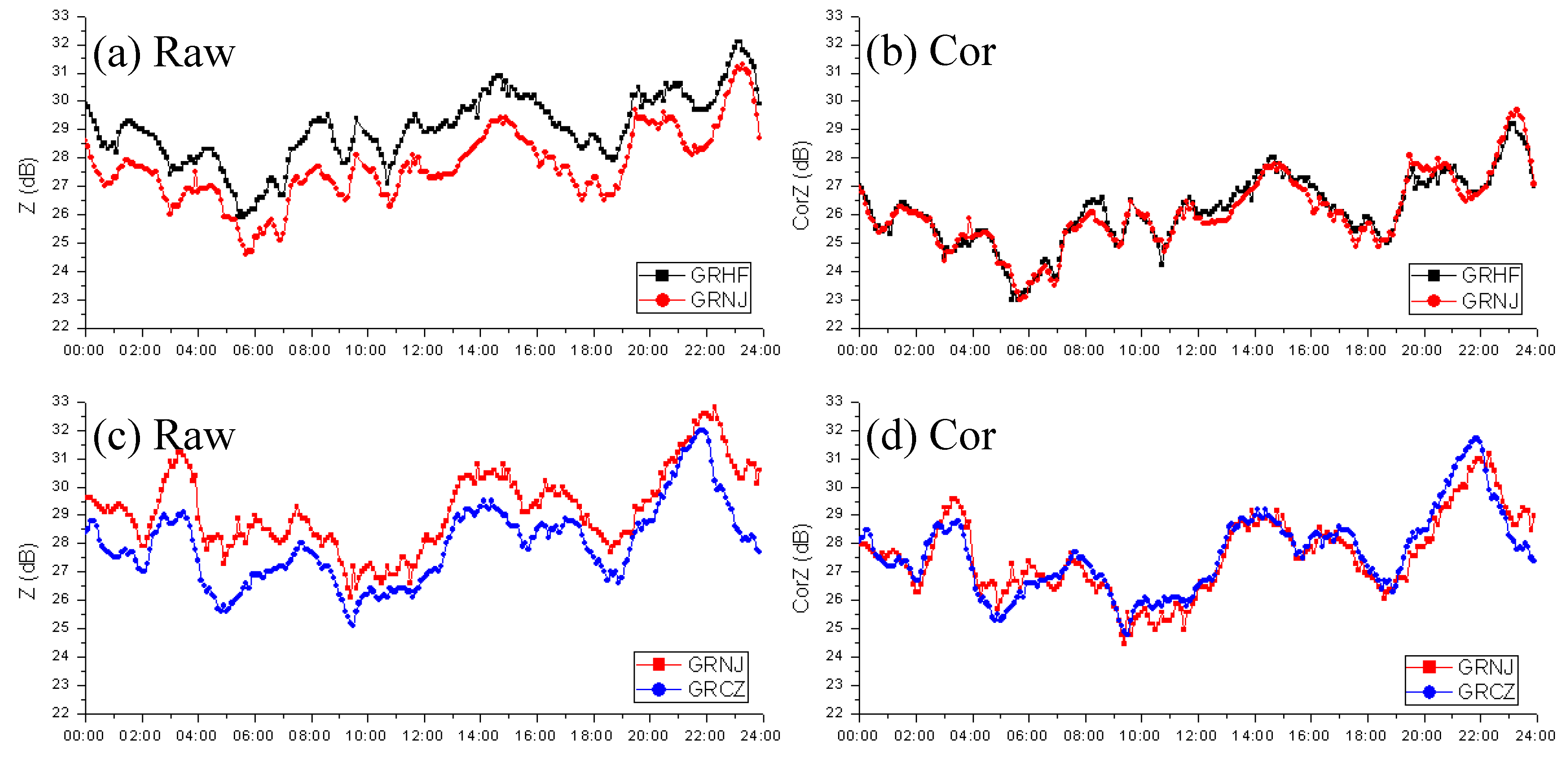
4.3. Spatial Continuity of Reflectivity Factor

The consistency in the reflectivity factor in the overlapping area between two adjacent radars is the premise to ensure the spatial continuity of MGR-QPE. The three radars had totally two overlapping areas of GRHF-GRNJ and GRCZ-GRNJ, respectively (Figure 1). The reflectivity differences were analyzed at the interval of 6 min (Figure 8,

Table 1. Reflectivity differences in overlapping areas of adjacent GRs.

Date/No.	Rain Type		Z Difference (dB)
			|GRHF-GRNJ|	|GRCZ-GRNJ|
05-09	Light Rain	RAW	3.29	2.69
		COR	0.26	0.25
07-02	Mei-yu	RAW	1.40	0.40
		COR	0.42	0.40
09-15	Typhoon	RAW	1.84	0.73
		COR	0.34	0.47
09-29	Frontal Heavy Rain	RAW	1.33	1.25
		COR	0.25	0.46
Average		RAW	1.62
		COR	0.36

). From 00:00 to 24:00 on 29 September 2016, the Z values of any two adjacent radars nearly changed similarly with time, but were different in values (Figure 8a,c), indicating the presence of obvious reflectivity differences among the three radars and the Z values were spatially discontinuous. After correction by M-ABCD, the outlines in the reflectivity factors of adjacent radars were gradually superposed and the differences significantly decreased (Figure 8b,d), indicating the Z values of multiple radars became more continuous. Quantitative analysis in Table 1 showed that differences in reflectivity factors in GRHF-GRNJ and GRCZ-GRNJ significantly decreased, especially for the case 05-09 in GRHF-GRNJ. The mean difference in the overlapping areas of the four precipitation events after correction decreased by 78% from 1.62 to 0.36 dB.

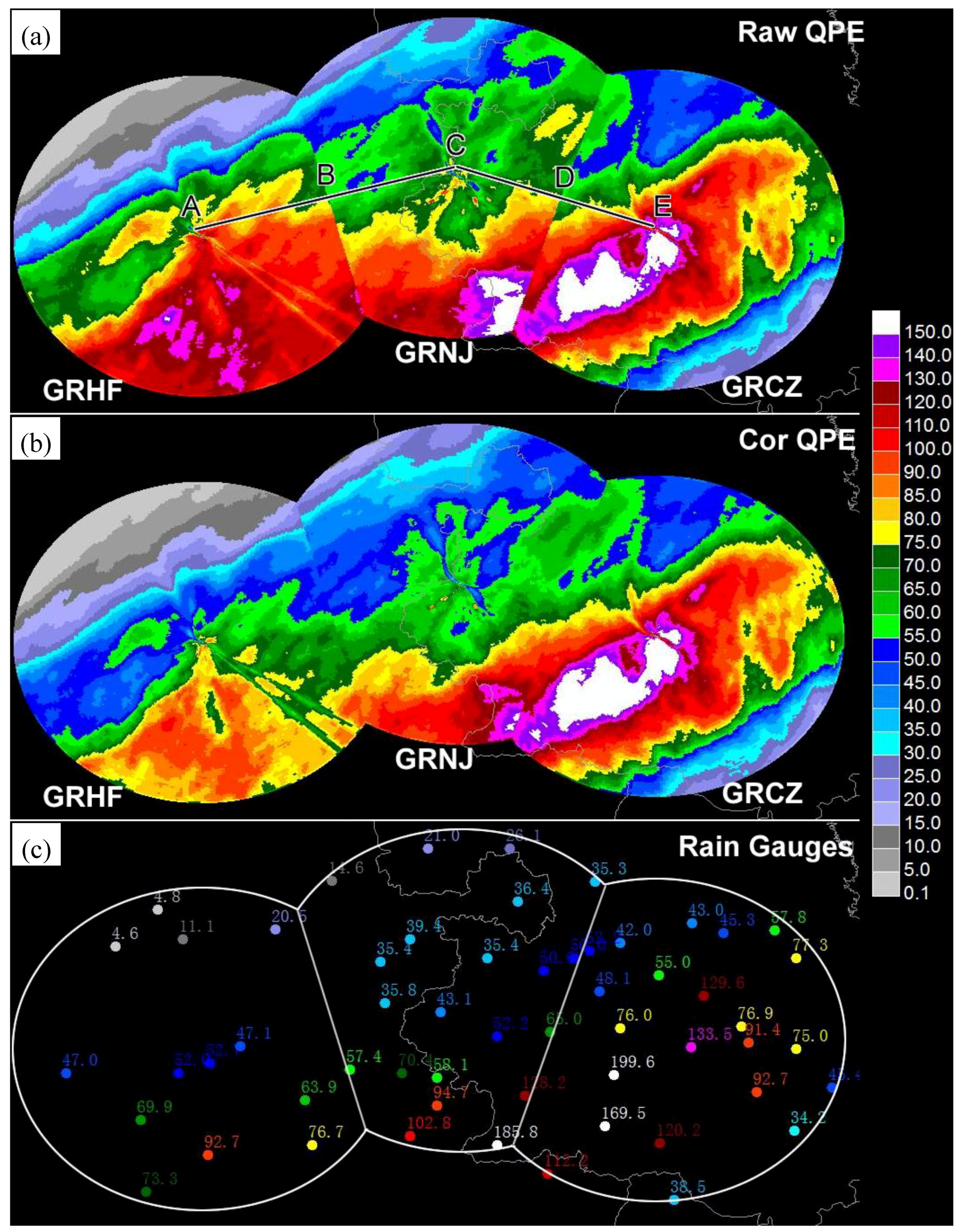
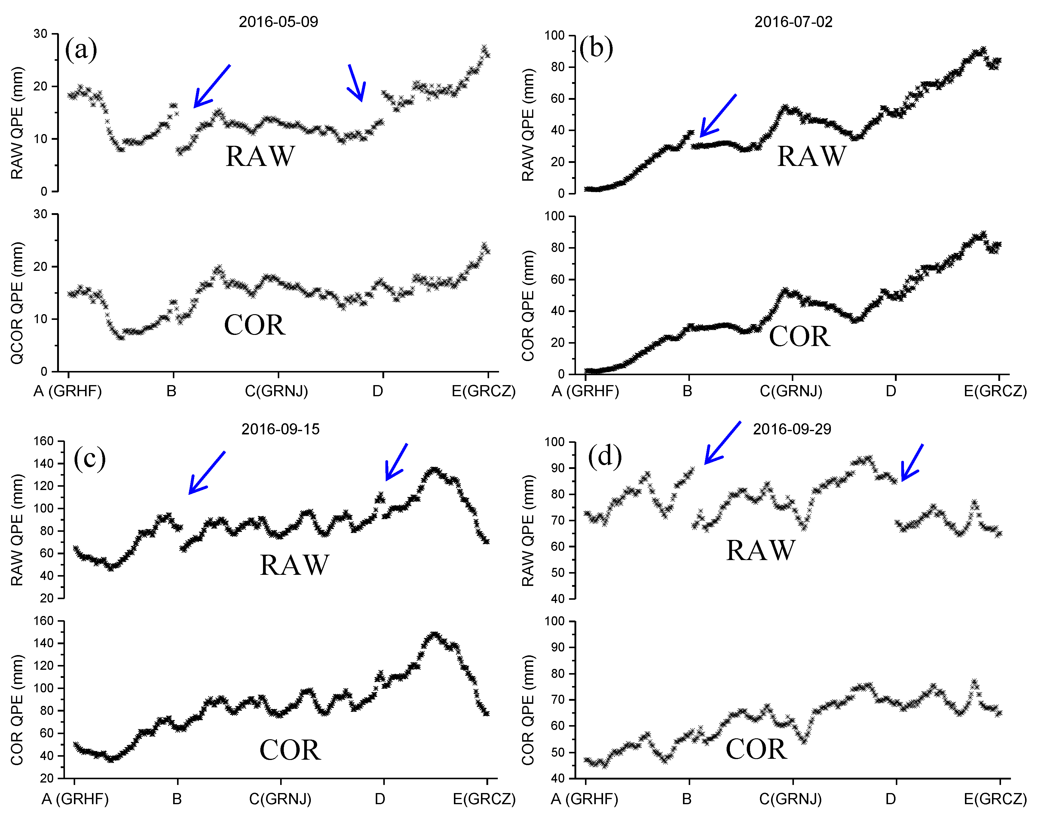
4.4. Spatial Continuity of MGR-QPE

The formula of $Z^{(\ell )}=200R^{1.6}$ [47] was used to get the rain rate $R$ (mm/h) of Mosaic Reflectivity of the three GRs, and $R$ was accumulated daily rainfall for 24 h. $Z^{(\ell )}$ is the reflectivity factor in linear unit and its relation with the reflectivity factor in logarithmic unit is $Z=10{\log }_{10}(Z^{(\ell )})$. $Z^{(\ell )}=200R^{1.6}$ is the stratiform estimation relation of Chinese operational radars. Stricter methods should use different estimation relations for stratiform and convective precipitations [48]. However, in this study, the four events were mainly stratiform precipitation without much convective precipitation embedded, and thus here only a single relation $Z^{(\ell )}=200R^{1.6}$ was used. The accumulated 24 h precipitation on 29 September 2016 observed by MGR-QPE is shown in Figure 9. Clearly, at the equidistance line between two adjacent radars, the original MGR-QPE showed evident leap (discontinuity) (Figure 9a). Precipitation estimations from different radars ranked in the order of GRHF > GRNJ > GRCZ, indicating the same precipitation area and the same estimated precipitation relation, but due to differences in calibration errors, the QPE differed. The QPE from M-ABCD was more continuous spatially, and the estimated precipitation at the equidistance line between radars was more similar. Compared with the gauge-based data (Figure 9c), the original QPE estimated from GRHF and GRNJ were obviously larger. The QPE of GRHF contained about a 1/3 zone with precipitation >100mm and maximum >130 mm, but the measured data were mostly between 50 and 80 mm, with the maximum being 92.7 mm. Similarly, the QPE were also overestimated by GRNJ. The QPE from GRCZ were not largely different from the rain gauges. After correction, QPE in Figure 9b were more reasonable.

Along the line A-B-C-D-E in Figure 9a, the MGR-QPE horizontal profiles of the four cases were plotted (Figure 10). B is the midpoint between GRHF and GRNJ, D is the midpoint between GRNJ and GRCZ, and the original profiles marked by blue arrows are spatially discontinuous. On the original QPE in Figure 10, spatial discontinuity appeared at B and D (except D in case 07-02), where the precipitation profiles were fractured. Such discontinuity disappeared on the corrected profiles, which became more natural and continuous. The statistics of QPE differences in the overlapping areas between adjacent radars are listed in

Table 2. Differences of 24h accumulated QPE in overlapping areas of adjacent GRs.

Date/No.	Data Type	24h QPE Difference (mm)
		|GRHF-GRNJ|	|GRCZ-GRNJ|
05-09	RAW	6.7	3.9
	COR	2.4	0.9
07-02	RAW	6.9	0.1
	COR	1.3	0.1
09-15	RAW	13.9	12.2
	COR	1.3	5.7
09-29	RAW	19.9	16.4
	COR	2.2	0.1
Average	RAW	10.0
	COR	1.8

. Using the M-ABCD, the differences of QPE at the two overlapping areas GRHF-GRNJ and GRCZ-GRNJ were both significantly reduced, especially in the case 09-29 in GRHF-GRNJ where the differences decreased from 19.9 to 2.2 mm. The mean differences of QPE in the four precipitation events decreased by about 82% from 10.0 to 1.8 mm, indicating the bias-corrected MGR-QPE was significantly more spatially coherent.

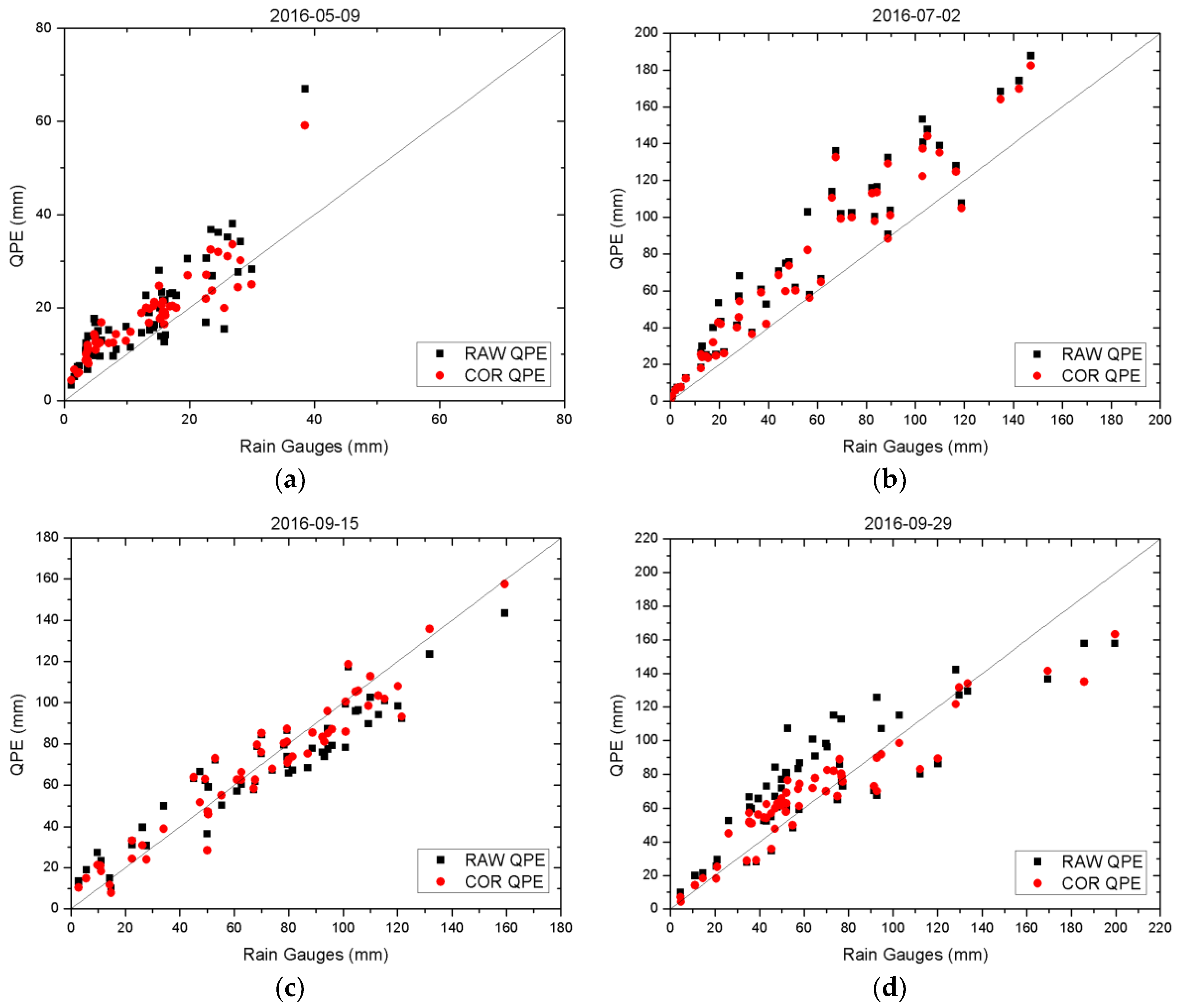
4.5. Accuracy of MGR-QPE

Based on the data measured by the 56 operational rain gauges (Figure 1), the MGR-QPE errors before and after correction were systematically evaluated (Figure 11,

Table 3. Error statistics of 24 h accumulated MGR-QPE.

Date/No.	Data Type	<Rain Gauge> (mm)	<QPE> (mm)	Correlation Coefficient	NE	RMSE (mm)
05-09	RAW	13.3	18.7	0.85	0.47	7.8
	COR		18.2	0.91	0.41	6.2
07-02	RAW	53.4	74.3	0.95	0.40	26.8
	COR		70.0	0.96	0.32	22.1
09-15	RAW	69.5	67.1	0.94	0.16	13.1
	COR		68.9	0.96	0.11	9.9
09-29	RAW	65.5	75.8	0.86	0.30	23.6
	COR		67.7	0.94	0.18	15.6

Note: <X> represents the average of X; NE = <|QPE − Gauge|>/<Gauge>; RMSE = <Bias²>^0.5.

). Clearly, the scattered points after correction are closer to the diagonal line (best fit line) and were more consistent with the gauge-observed data (Figure 11). The two precipitation events on 09-15 and 09-29 were significantly improved, and the two ones on 05-09 and 07-02 were slightly improved. Precipitation estimations on 07-02 were still large after the correction, which might be attributed to the estimation model errors of Z–R relation. The statistics of MGR-QPE and measured rainfall were listed in Table 3. The difference in calibration errors among radars before correction led to different biases in precipitation estimations, and thus, the correlation coefficient between MGR-QPE and rain gauges was not the optimal. Since the calibration errors and space discontinuity were addressed, the correlation coefficient after bias-correction increased by 0.01 (case 07-02) and 0.08 (case 09-29), respectively. Similarly, the Normalized Absolute Error (NE) and Root Mean-Square Error (RMSE) were both significantly reduced after the correction, as NE declined by 0.05 mm (case 09-15) to 0.12 mm (case 09-29), while RMSE decreased by 1.6 mm (case 05-09) to 8.0 mm (case 09-29). The above results suggest that the M-ABCD method significantly eliminates the spatial discontinuity of MGR-QPE, and also improves the associated data accuracy.

5. Summary and Discussion

Spatial discontinuity of QPE due to radar calibration errors is a concern on MGR-QPE [49]. The precipitation estimation model of single polarization radar is expressed as $Z=10{\log }_{10}a+10b{\log }_{10}R$, (Z in dBZ, R in $\mathrm{mm}\cdot {\mathrm{h}}^{-1}$). When the model errors are ignored, the equation is differentiated to $\Delta Z=\frac{10b}{\ln 10}\frac{\Delta R}{R}$. $\Delta Z$ is the calibration error in dB. The relative error $\frac{\Delta R}{R}$ of precipitation estimation is linearly related with the calibration error $\Delta Z$. If $b$ is limited to 1.2–1.6, when $\Delta Z$ is 3.0 dB, $\frac{\Delta R}{R}$ will be up to 40%~60%. Similarly, we have $\frac{\partial a}{\partial Z}=\frac{a\ln 10}{10}>0.2a$. Generally, the precipitation estimation relations set $a\ge 200$, and then $\frac{\partial a}{\partial Z}>40$; thus, the calibration error $\Delta Z$ would largely affect coefficient $a$. Conversely, since $\frac{\partial b}{\partial Z}=\frac{1}{10{\log }_{10}(R)}$, then when $R\ge 2.5\mathrm{mm}\cdot {\mathrm{h}}^{-1}$, we have $\frac{\partial b}{\partial Z}<0.3$, indicating the $\Delta Z$ only slightly affects $b$. Taken together, the calibration error mainly affects the relative errors $\frac{\Delta R}{R}$ of precipitation estimation or the coefficient $a$ of precipitation estimation relation. When single GR was used in precipitation estimation, the impact of calibration errors could be reduced by adjusting $a$. For MGR-QPE, it was difficult to determine and use different coefficients to different radars, and usually the same precipitation estimation model with the same coefficients was adopted. However, the calibration errors vary among radars, which led to different relative errors in the various rainfall zones. This results in spatial discontinuity of MGR-QPE and lower quality of QPE.

A new M-ABCD method was proposed in this study, where and the calibration errors of several GRs were synchronously corrected with GPM/KuPR as the standard reference, so as to generate Mosaic Reflectivity and MGR-QPE products with spatial continuity. Four typical precipitation events in the year 2016 in the downstream of the Yangtze River were selected to evaluate the spatial continuity and associated QPE accuracy with regard to three operational radars. (1) the three radars, despite periodic maintenance and hardware calibration, suffered from severe calibration errors. The MGR-QPE products were obviously discontinuous in space before adjustment; (2) the differences of Z and QPE in the overlapping areas between adjacent radars were reduced by 78% and 82% after correction, respectively; (3) the MGR-QPE data show more consistent gauge observations after correction, with regard to the correlation coefficient increased by 0.01–0.08, the normalized absolute error decreased by 0.05–0.12, and the RMSE declined by 1.6–8.0 mm.

Compared with the TRMM/PR-based single-GR correction method (e.g., ABCD), M-ABCD has three advantages: (1) ABCD belongs to single-GR correction and could reduce calibration errors, but not able to ensure spatial continuity, while M-ABCD is a multiple-GR correction method that can simultaneously reduce calibration errors and spatial discontinuity; (2) ABCD is based on TRMM/PR, but since TRMM stopped service, only historical data before 2015 were available. On the contrary, M-ABCD based on GPM/KuPR is feasible for the new GR data after 2015; (3) ABCD requires TRMM/PR and single-GR have some overlapping areas, and thus, there are few matched events. On the contrary, M-ABCD requires KuPR have some overlapping zones with any of multiple GRs, and thus, there are more matched events. Compared with inter-calibration of adjacent GRs methods, such as Radar Reflectivity Comparison Tool (http://rrct.nwc.ou.edu/) or the method of Seo et al. [41], the relative correction of M-ABCD is similar to that of Seo et al. [41], but the absolute correction is different. Seo et al. [41] suggested the usage of rain gauges as a reference for absolute correction, since the reflectivity factor and precipitation rate are not the same observations, their relationship is based on statistics, which account for the very large difficulty and uncertainty. M-ABCD compares the reflectivities of KuPR and GR, which is more direct and reliable.

M-ABCD also has some limitations: (1) Although M-ABCD has more available events than single GR, there are still insufficient to correct GRs in real time. Thus, we could only use the result of one time to represent the average value in a period, and its feasibility needs more discussion. Ryzhkov et al. [50] noted the calibration errors of operational radars were stable within long time, but may also change sometimes. Seo et al. [41] also found the abrupt changes in the two years of WSR-88D calibration errors. If the calibration errors changed suddenly, the representativeness was weakened, and the corrected results would be very wrong; (2) If the matchup events of KuPR and GRs are convective precipitation, the M-ABCD method is not reliable because STEP6 (Figure 4) will exclude all convective data. An alternative approach is to identify a matchup stratiform event at the nearest time, and use its $\Delta Z$ from M-ABCD to calibrate this convective precipitation. If there are no abrupt changes for calibration errors in the interval between the two matchup events, M-ABCD would improve the convective precipitation. 3) This approach was proposed with the S-band GR data, which might not be feasible for the C-band or X-band GRs. As the calibration errors and attenuation coexist, it is difficult to calibrate either of them. Thus, the M-ABCD method is further updated with the consideration of the attenuation correction algorithm [51].

References

1. Gou, Y.; Ma, Y.; Chen, H.; Wen, Y. Radar-derived Quantitative Precipitation Estimation in Complex Terrain over the Eastern Tibetan Plateau. Atmos. Res. 2018, 203, 286–297. [Google Scholar] [CrossRef]
2. Wilson, J.W.; Brandes, E.A. Radar Measurement of Rainfall—A Summary. Bull. Am. Meteorol. Soc. 1979, 60, 1048–1058. [Google Scholar] [CrossRef] [Green Version]
3. Zhang, J.; Qi, Y.; Kingsmill, D.; Howard, K. Radar-Based Quantitative Precipitation Estimation for the Cool Season in Complex Terrain: Case Studies from the NOAA Hydrometeorology Testbed. J. Hydrometeorol. 2012, 13, 1836–1854. [Google Scholar] [CrossRef]
4. Ulbrich, C.W.; Lee, L.G. Rainfall Measurement Error by WSR-88D Radars due to Variations in Z–R Law Parameters and the Radar Constant. J. Atmos. Ocean Technol. 1999, 16, 1017–1024. [Google Scholar] [CrossRef]
5. Rosenfeld, D.; Ulbrich, C.W. Cloud Microphysical Properties, Processes, and Rainfall Estimation Opportunities. In Radar and Atmospheric Science: A Collection of Essays in Honor of David Atlas; Wakimoto, R.M., Srivasva, R.C., Eds.; Springer: Berlin, Germany, 2003; pp. 237–258. [Google Scholar]
6. Seo, B.-C.; Cunha, L.K.; Krajewski, W.F. Uncertainty in Radar-Rainfall Composite and its Impact on Hydrologic Prediction for the Eastern Iowa Flood of 2008. Water Resour. Res. 2013, 49, 2747–2764. [Google Scholar] [CrossRef]
7. Brandes, E.A.; Vivekanandan, J.; Wilson, J.W. A Comparison of Radar Reflectivity Estimates of Rainfall from Collocated Radars. J. Atmos. Ocean. Technol. 1999, 16, 1264–1272. [Google Scholar] [CrossRef]
8. Smith, J.A.; Seo, D.J.; Baeck, M.L.; Hudlow, M.D. An Intercomparison Study of NEXRAD Precipitation Estimates. Water Resour. Res. 1996, 32, 2035–2045. [Google Scholar] [CrossRef]
9. Gourley, J.J.; Kaney, B.; Maddox, R.A. Evaluating the Calibration of Radars: A Software Approach. In Proceedings of the 31st International Conference on Radar Meteorology, Seattle, WA, USA, 5–12 August 2003. P3C.1. [Google Scholar]
10. You, C.H.; Kang, M.Y.; Lee, D.I.; Lee, J.T. Approaches to Radar Reflectivity Bias Correction to Improve Rainfall Estimation in Korea. Atmos. Meas. Tech. 2016, 9, 2043–2053. [Google Scholar] [CrossRef]
11. Xiao, Y.; Liu, L. Study of Methods for Interpolating Data from Weather Radar Network to 3-D Grid and Mosaics (in Chinese). Acta Meteorol. Sin. 2006, 64, 647–657. [Google Scholar] [CrossRef]
12. Doviak, R.J.; Zrnic, D.S. Doppler Radar and Weather Observations; Academic Press: Cambridge, MA, USA, 1993; 562p. [Google Scholar]
13. Atlas, D. Radar Calibration: Some Simple Approaches. Bull. Am. Meteorol. Soc. 2002, 83, 1313–1316. [Google Scholar] [CrossRef]
14. Vaccarono, M.; Bechini, R.; Chandrasekar, C.V.; Cremonini, R.; Cassardo, C. An Integrated Approach to Monitoring the Calibration Stability of Operational Dual-Polarization Radars. Atmos. Meas. Tech. 2016, 9, 5367–5383. [Google Scholar] [CrossRef]
15. Kozu, T.; Kawanishi, T.; Kuroiwa, H.; Kojima, M.; Oikawa, K.; Kumagai, H.; Okamoto, K.; Okumura, M.; Nakatsuka, H.; Nishikawa, K. Development of Precipitation Radar Onboard the Tropical Rainfall Measuring Mission (TRMM) Satellite. IEEE Trans. Geosci. Remote Sens. 2001, 39, 102–116. [Google Scholar] [CrossRef]
16. Takahashi, N.; Kuroiwa, H.; Kawanishi, T. Four Year Result of External Calibration for Precipitation Radar (PR) of the Tropical Rainfall Measuring Mission (TRMM) Satellite. IEEE Trans. Geosci. Remote Sens. 2003, 41, 2398–2403. [Google Scholar] [CrossRef]
17. Kim, J.; Ou, M.; Park, J.; Morris, K.R.; Schwaller, M.R.; Wolff, D.B. Global Precipitation Measurement (GPM) Ground Validation (GV) Prototype in the Korean Peninsula. J. Atmos. Ocean. Technol. 2014, 31, 1902–1921. [Google Scholar] [CrossRef]
18. Han, J.; Chu, Z.; Wang, Z.; Xu, D.; Li, N.; Kou, L.; Xu, F.; Zhu, Y. The Establishment of Optimal Ground-Based Radar Datasets by Comparison and Correlation Analyses with Space-Borne Radar Data. Meteorol. Appl. 2017, 25, 161–170. [Google Scholar] [CrossRef]
19. Liao, L.; Meneghini, R.; Iguchi, T. Comparisons of Rain Rate and Reflectivity Factor Derived from the TRMM Precipitation Radar and the WSR-88D over the Melbourne, Florida, Site. J. Atmos. Ocean. Technol. 2001, 18, 1959–1974. [Google Scholar] [CrossRef]
20. Liao, L.; Meneghini, R. Validation of TRMM Precipitation Radar through Comparison of Its Multiyear Measurements with Ground-Based Radar. J. Appl. Meteorol. Climatol. 2009, 48, 804–817. [Google Scholar] [CrossRef] [Green Version]
21. Anagnostou, E.N.; Morales, C.A.; Dinku, T. The Use of TRMM Precipitation Radar Observations in Determining Ground Radar Calibration Biases. J. Atmos. Ocean. Technol. 2001, 18, 616–628. [Google Scholar] [CrossRef]
22. Wang, J.X.; Wolff, D.B. Comparisons of Reflectivities from the TRMM Precipitation Radar and Ground-Based Radars. J. Atmos. Ocean. Technol. 2009, 26, 857–875. [Google Scholar] [CrossRef] [Green Version]
23. Chu, Z.; Yin, Y.; Gu, S. Characteristics of Velocity Ambiguity for CINRAD-SA Doppler Weather Radars. Asia-Pac. J. Atmos. Sci. 2014, 50, 221–227. [Google Scholar] [CrossRef]
24. Wu, T.; Wan, Y.; Wo, W.; Leng, L. Design and Application of Radar Reflectivity Quality Control Algorithm in SWAN (in Chinese). Meteorol. Sci. Technol. 2013, 41, 809–817. [Google Scholar] [CrossRef]
25. Tokay, A.; Wolff, D.B.; Petersen, W.A. Evaluation of the New Version of Laser-Optical Disdrometer, OTT Parsivel2. J. Atmos. Ocean. Technol. 2014, 31, 1276–1288. [Google Scholar] [CrossRef]
26. Shen, Y.; Xiong, A. Validation and Comparison of a New Gauge-Based Precipitation Analysis over Mainland China. Int. J. Climatol. 2016, 36, 252–265. [Google Scholar] [CrossRef]
27. Hou, A.Y.; Kakar, R.K.; Neeck, S.; Azarbarzin, A.A.; Kummerow, C.D.; Kojima, M.; Oki, R.; Nakamura, K.; Iguchi, T. The Global Precipitation Measurement Mission. Bull. Am. Meteor. Soc. 2014, 95, 701–722. [Google Scholar] [CrossRef] [Green Version]
28. Meneghini, R.; Kim, H.; Liao, L.; Jones, J.A.; Kwiatkowski, J.M. An Initial Assessment of the Surface Reference Technique Applied to Data from the Dual-Frequency Precipitation Radar (DPR) on the GPM Satellite. J. Atmos. Ocean. Technol. 2015, 32, 2281–2296. [Google Scholar] [CrossRef]
29. Seto, S.; Iguchi, T. Intercomparison of Attenuation Correction Methods for the GPM Dual-Frequency Precipitation Radar. J. Atmos. Ocean. Technol. 2015, 32, 915–926. [Google Scholar] [CrossRef]
30. Iguchi, T.; Kozu, T.; Meneghini, R.; Awaka, J.; Okamoto, K. Rain-Profiling Algorithm for the TRMM Precipitation Radar. J. Appl. Meteorol. 2000, 39, 2038–2052. [Google Scholar] [CrossRef]
31. Iguchi, T.; Seto, S.; Awaka, J.; Meneghini, R.; Kubota, T. Performance of the Dual-frequency Precipitation Radar on the GPM core satellite. Geophys. Res. Abstr. 2016, 18, 11581. [Google Scholar]
32. Bringi, V.N.; Chandrasekar, V.; Hubbert, J.; Gorgucci, E.; Randeu, W.L.; Schoenhuber, M. Raindrop Size Distribution in Different Climatic Regimes from Disdrometer and Dual-Polarized Radar Analysis. J. Atmos. Sci. 2003, 60, 354–365. [Google Scholar] [CrossRef]
33. Cao, Q.; Zhang, G. Errors in Estimating Raindrop Size Distribution Parameters Employing Disdrometer and Simulated Raindrop Spectra. J. Appl. Meteorol. Clim. 2009, 48, 406–425. [Google Scholar] [CrossRef]
34. Waterman, P.C. Matrix Formulation of Electromagnetic Scattering. Proc. IEEE 1965, 53, 805–812. [Google Scholar] [CrossRef]
35. Mishchenko, M.I.; Travis, L.D.; Mackowski, D.W. T-Matrix Computations of Light Scattering by Nonspherical Particles: A review. J. Quant. Spectrosc. Radiat. Transf. 1996, 55, 535–575. [Google Scholar] [CrossRef]
36. Beard, K.V.; Chuang, C. A New Model for The Equilibrium Shape of Raindrops. J. Atmos. Sci. 1987, 44, 1509–1524. [Google Scholar] [CrossRef]
37. Kalogiros, J.; Anagnostou, M.N.; Anagnostou, E.N.; Montopoli, M.; Picciotti, E.; Marzano, F.S. Optimum Estimation of Rain Microphysical Parameters from X-band Dual-Polarization Radar Observables. IEEE Trans. Geosci. Remote Sens. 2013, 51, 3063–3076. [Google Scholar] [CrossRef]
38. Awaka, J.; Le, M.D.; Chandrasekar, V.; Yoshida, N.; Higashiuwatoko, T.; Kubota, T.; Iguchi, T. Rain Type Classification Algorithm Module for GPM Dual-Frequency Precipitation Radar. J. Atmos. Ocean. Technol. 2016, 33, 1887–1898. [Google Scholar] [CrossRef]
39. Liao, L.; Meneghini, R. Changes in the TRMM Version-5 and Version-6 Precipitation Radar Products due to Orbit Boost. J. Meteorol. Soc. Jpn. 2009, 87, 93–107. [Google Scholar] [CrossRef]
40. Le, M.; Chandrasekar, V.; Biswas, S. Evaluation and Validation of GPM Dual-Frequency Classification Module after Launch. J. Atmos. Ocean. Technol. 2016, 33, 2699–2716. [Google Scholar] [CrossRef]
41. Seo, B.-C.; Krajewski, W.F.; Smith, J.A. Four-Dimensional Reflectivity Data Comparison between Two Ground-Based Radars: Methodology and Statistical Analysis. Hydrol. Sci. J. 2014, 59, 1312–1326. [Google Scholar] [CrossRef]
42. Cressman, G.P. An Operational Objective Analysis System. Mon. Weather Rev. 1959, 81, 367–374. [Google Scholar] [CrossRef]
43. Schwaller, M.R.; Morris, K.R. A Ground Validation Network for the Global Precipitation Measurement Mission. J. Atmos. Ocean. Technol. 2011, 28, 301–319. [Google Scholar] [CrossRef] [Green Version]
44. Derin, Y.; Anagnostou, E.N.; Anagnostou, M.N.; Kalogiros, J.; Casella, D.; Marra, A.C.; Panegrossi, G.; Sanò, P. Passive Microwave Rainfall Error Analysis using High-Resolution X-band Dual-Polarization Radar Observations in Complex Terrain. IEEE Trans. Geosci. Remote Sens. 2018, 56, 2565–2586. [Google Scholar] [CrossRef]
45. Bolen, S.M.; Chandrasekar, V. Quantitative Cross Validation of Space-based and Ground-based Radar Observations. J. Appl. Meteorol. 2000, 39, 2071–2079. [Google Scholar] [CrossRef]
46. Park, S.; Jung, S.; Lee, G. Cross-validation of TRMM PR Reflectivity Profiles Using 3-D Reflectivity Composite from the Ground-Based Radar Network over the Korean Peninsula. J. Hydrometeorol. 2015, 16, 668–687. [Google Scholar] [CrossRef]
47. Marshall, J.S.; Hitschfeld, W.; Gunn, K.L.S. Advances in Radar Weather. Adv. Geophys. 1955, 2, 1–56. [Google Scholar] [CrossRef]
48. Zhang, J.; Howard, K.; Langston, C.; Vasiloff, S.; Kaney, B.; Arthur, A.; Cooten, S.V.; Kelleher, K.; Kitzmiller, D.; Ding, F.; et al. National Mosaic and Multi-Sensor QPE (NMQ) System: Description, Results, and Future Plans. Bull. Am. Meteorol. Soc. 2011, 92, 1321–1338. [Google Scholar] [CrossRef] [Green Version]
49. Hong, Y.; Gourley, J.J. Radar Hydrology: Principles, Models, and Applications, 1st ed.; CRC Press: Boca Raton, FL, USA, 2014; pp. 17–19. [Google Scholar]
50. Ryzhkov, A.V.; Giangrande, S.E.; Melnikov, V.M. Calibration Issues of Dual-Polarization Radar Measurements. J. Atmos. Ocean. Technol. 2005, 22, 1138–1155. [Google Scholar] [CrossRef]
51. Kalogiros, J.; Anagnostou, M.N.; Anagnostou, E.N.; Montopoli, M.; Picciotti, E.; Marzano, F.S. Evaluation of a New Polarimetric Algorithm for Rain-Path Attenuation Correction of X-Band Radar Observations Against Disdrometer. IEEE Trans. Geosci. Remote Sens. 2014, 52, 1369–1380. [Google Scholar] [CrossRef]
Figure 1. The locations and 100 km radius coverages of three ground radars, locations of operational rain gauges and a disdrometer, schematic coverage of GPM/KuPR.
Hydrology 05 00048 g001
Figure 2. Simulated reflectivities from DSD spectra measurements versus observed reflectivities from KuPR. Scatter plot (a) and frequency distribution (b).
Hydrology 05 00048 g002
Figure 3. Reflectivity relations between Ku and S band. Liao(Rain) and Liao(Snow) curves are from Liao and Meneghini [39]. DSD(Rain) curve is from DSD calculation.
Hydrology 05 00048 g003
Figure 4. Flow chart of the proposed M-ABCD method. Ellipses indicate radar data or match-up datasets, and rectangles indicate processing steps. STEP1 is correction for spatial discontinuity, and STEP2–STEP8 are correction for calibration errors.
Hydrology 05 00048 g004
Figure 5. Correlation coefficient (black) and standard deviation (blue) of match-up dataset. STEP2 represents the original match-up dataset of Mosaic Reflectivity and KuPR. STEP3–STEP6 represent the match-up dataset output from STEP3 to STEP6.
Hydrology 05 00048 g005
Figure 6. Scatter plot of KuPR and GR Mosaic Reflectivity. The blue line is the fitting line. (a) Original match-up dataset from STEP2. (b) Optimal match-up dataset from STEP6.
Hydrology 05 00048 g006
Figure 7. Raw and corrected reflectivity distribution for 29 September 2016 precipitation event. (a) GRHF. (b) GRNJ. (c) GRCZ. (d) Mosaic Reflectivity. KuPR(S) indicates KuPR reflectivities which were adjusted to S-Band by Radar Frequency Corrections.
Hydrology 05 00048 g007
Figure 8. Raw reflectivity profile (a,c) and corrected reflectivity profile (b,d) for 2016-09-29 precipitation event. (a,b) Average reflectivity in GRHF and GRNJ overlapping area. (c,d) Average reflectivity in GRNJ and GRCZ overlapping area.
Hydrology 05 00048 g008
Figure 9. Raw (a), corrected (b), measured (c) 24 h accumulated rainfall for 29 September 2016 precipitation event.
Hydrology 05 00048 g009
Figure 10. Raw and corrected QPE profile along the A-B-C-D-E line of Figure 9a. B is the midpoint of GRHF and GRNJ, D is the midpoint of GRNJ and GRCZ. Blue arrows indicate spatial discontinuity. (ad) indicate 05-09, 07-02, 09-15 and 09-29 precipitation events, respectively.
Hydrology 05 00048 g010
Figure 11. Raw and corrected MGR-QPE versus measured rainfall of rain gauges. (ad) indicate 05-09, 07-02, 09-15 and 09-29 precipitation events, respectively.
Hydrology 05 00048 g011