Projected Changes of Precipitation IDF Curves for Short Duration under Climate Change in Central Vietnam

Abstract

In future years, extreme weather events are expected to frequently increase due to climate change, especially in the combination of climate change and events of El Niño–Southern Oscillation. This pays special attention to the construction of intensity–duration–frequency (IDF) curves at a tempo-spatial scale of sub-daily and sub-grid under a context of climate change. The reason for this is that IDF curves represent essential means to study effects on the performance of drainage systems, damps, dikes and reservoirs. Therefore, the objective of this study is to present an approach to construct future IDF curves with high temporo-spatial resolutions under climate change in central Vietnam, using the case of VuGia-ThuBon. The climate data of historical and future from a regional climate model RegCM4 forced by three global models MPI-ESM-MR, IPSL-CM5A-LR and ICHEC-EC-EARTH are used to re-grid the resolution of 10 km × 10 km grid spacing from 25 km × 25 km on the base of bilinear interpolation. A bias correction method is then applied to the finest resolution of a hydrostatic climate model for an ensemble of simulations. Furthermore, the IDF curves for short durations of precipitation are constructed for the historical climate and future climates under two representative concentration pathway (RCP) scenarios, RCP4.5 and RCP8.5, based on terms of correlation factors. The major findings show that the projected precipitation changes are expected to significantly increase by about 10 to 30% under the scenarios of RCP4.5 and RCP8.5. The projected changes of a maximum of 1-, 2-, and 3-days precipitation are expected to increase by about 30–300 mm/day. More importantly, for all return periods (i.e., 10, 20, 50, 100, and 200 years), IDF curves completely constructed for short durations of precipitation at sub-daily show an increase in intensities for the RCP4.5 and RCP8.5 scenarios.

1. Introduction

To date, changes in climate are acknowledged by a large part of the scientific community in a wide range of different fields. The Intergovernmental Panel on Climate Change (IPCC) AR4 specifically emphasized the rise of the average global surface temperature by up to +0.074 °C per year from 1906 to 2000 [1]. Later, the IPCC AR5 indicated that the average temperature trend is estimated equal to +0.85 °C, with a degree of uncertainty ranging between +0.65 °C and +1.06 °C, over the period 1880–2012 on a global scale [2]. Additionally, average temperature is estimated to have increased by +0.78 °C during the last decade (2003–2012). More importantly, according to the IPCC AR5 report, an increase in mean temperature will continue for the 2016–2035 period [2]. The report of IPCC AR5 showed that for average annual Northern Hemisphere temperatures, the period of time between 1983–2012 have been “very likely the warmest 30-year period of the last 800 years in the Northern Hemisphere”. In many land regions since about 1950s, the IPCC AR4 indicated there have been “likely” growths of the number of heavy precipitation events. The IPCC’s reports showed increases in the frequency of extreme precipitation events to be consistent with the growth of temperature and atmospheric water vapor over most land areas [1]. The IPCC AR5 showed an increase in the frequency of the heaviest precipitation during warmer years over the tropical oceans. In addition, annual precipitation over the tropical land areas of 30°S to 30°N is expected to have increased over the last decade. All these give rise to the questions as to whether and how this phenomenon on a grid scale shows its footstep on a sub-grid scale.

In recent decades, studies in dealing with precipitation events and its trends have enormously progressed [3,4,5,6]. On a regional scale, the precipitation trend has decreased in Asia [7,8]. In China, different trends have been shown in precipitation from region to region [9]. In the North China Plain and North Central China, a decrease in precipitation has observed; in the Southwest of China, no change in precipitation has been indicated. The findings of some studies over Thailand showed a trend toward wetter conditions of the magnitude of intense precipitation events [10]. On the domain of Vietnam, an analysis of trends of precipitation from 80 terrestrial observational stations over Vietnam has shown a decrease in precipitation in the north of 17°N latitude, meanwhile precipitation has increased in the South. Furthermore, precipitation has increased and decreased in the central regions and in the northern area of Vietnam, respectively [11]. In addition, insignificant trends have been demonstrated in the southern sub-region of Vietnam. The probability distributions of 20 extreme precipitation indices (e.g., maximums of 1 day, 3 days, and 5 days precipitation) have been studied for a limited mountain area in southern Vietnam [12]. Most of the above studies have mainly focused on large and/or regional scales without an emphasis on a sub-grid scale processes as well as sub-daily scale values.

Precipitation events play a central role in water and sustainable development and urban drainage systems. The reason for this is that the structures of hydrologic or/and hydraulic systems (e.g., storm water management, catch basins) are typically designed on the basic of local precipitation intensity–duration–frequency (IDF) curves. With an IDF curve, the time concentration or time structure of the precipitation is clearly depicted as introduced [13,14,15]. In other words, the frequency of occurrence of a storm with a specific intensity at different durations is quantified. In a norm, the construction of IDF curves is based on the annual maximum precipitation intensity characteristics. To do this, the requests of precipitation information at high tempo-spatial resolutions are very valuable. However, it is difficult to collect long records of short- and long-duration precipitation in most areas of developing countries like Vietnam. Besides that, traditionally, IDF curves are originated from a series of historical precipitation records with a temporal stationarity assumption of precipitation series. This means that the magnitude and frequency of historical precipitation are unchanged for the future [14]. Consequently, historical IDF curves cannot be used to represent the conditions of future climate, especial in a warmer climate. Under possible changes of climate, therefore, it is very crucial to find an approach to construct IDF curves at sub-grid and sub-daily scales.

In recent studies, future IDF curves are made on the basis of statistical downscaling methods with GCM outputs [16,17,18]. These studies, however, still concentrated on a horizontal resolution of between 100 km and 300 km and a temporal resolution ranging from daily to annual. Still, the grid size is too coarse to adequately represent convective precipitation, which is the primary process for the analysis of hydrologic and hydraulic systems. In Vietnam, particularly, there are few or even no studies in the construction of future IDF curves which explore methodologies at sub-grid and sub-daily scales under the context of climate change. Thus, the objective of this study is to: (1) project the possible changes of precipitation events (e.g., annual maximum 1, 2, 3 days precipitation) under the scenarios of RCP4.5 and RCP8.5; and (2) construct the future IDF curves for short duration of precipitation under a context of climate change (e.g., 1, 3, 6 h).

2. Materials and Methods

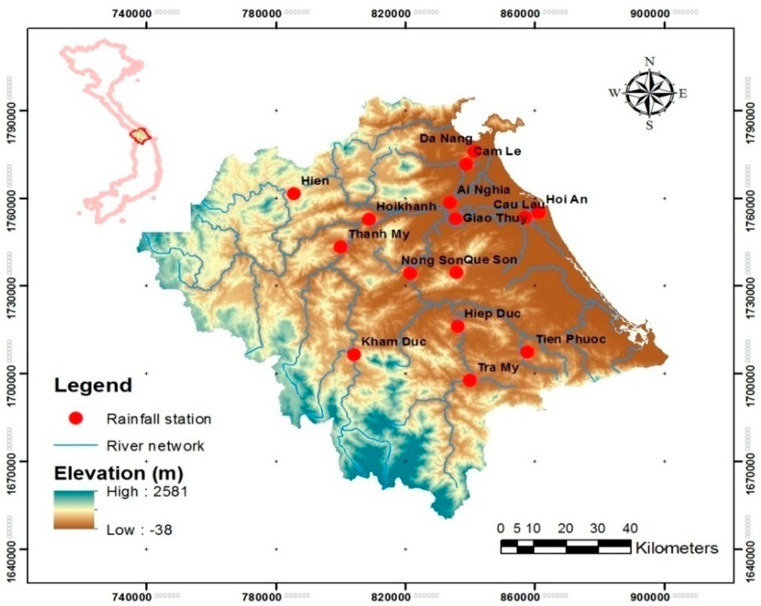
2.1. Description of the Case Study Area: Vu Gia-Thu Bon Basin

A plot basin, Vu Gia-Thu Bon (VG-TB), is selected in this study. It is located in central Vietnam, stretching from 6°55’ through 14°55’ and from 107°15’ through 108°24’, covering a total of area of approximately 12,577 km². The VG-TB basin is surrounded by two main provincial administrative territories Quang Nam and Da Nang. The basin is characterized by a steep topography and the altitude ranges from 0 m at the coast to 2598 m in elevation in the west (Figure 1).

2.2. Data

Hourly precipitation records are obtained from the Vietnam Hydro-Meteorological Data Center, which belongs to the Ministry of National Resources and Environment of Vietnam (MONRE), with a total of two meteorological stations (i.e., Tramy and Danang) as shown in Figure 1. These stations are national rain gauge stations in which Danang station provides the precipitation information for coastal area and Tramy station served for mountainous region. Data is available from 1990–2015 for hourly scales and from 1961–2016 (Danang station) and 1977–2016 (Tramy station) for daily scales. Besides that, other stations including Tienphuoc, Khamduc, Hiepduc, Hien, Thanhmy, Nongson, Queson, Hoikhanh, Ainghia, Giaothuy, Camle, Caulau, Hoikhanh are also popular rain gauge stations which are operated manually by a base of local volunteers. The locations of these stations can be seen in Figure 1. Data is generally available from 1977–2016. Use of the precipitation products from the Southeast Asia Regional Climate Downscaling/Coordinated Regional Climate Downscaling Experiment South East Asia (SEACLID-CORDEX South East Asia) is made. Future precipitation projections in the dataset for the 21st century are forced by prescribed levels of total radiative forcings determined by a cumulative measure of green house gas emissions, land use and air pollution. The radiative forcings are referred to as representative concentration pathways (RCPs). In this study, two greenhouse gas concentration scenarios, namely RCP4.5 and RCP8.5, are considered. The RCP4.5 is a stabilization scenario where total radiative forcing is stabilized before 2100 by employment of a range of technologies and strategies for reducing greenhouse gas emissions. The scenario drivers and technology options can be found in Clarke et al. [19]. Additional detail on the simulation of land use and terrestrial carbon emissions is given by Wise et al. [20]. Meanwhile, RCP8.5 is characterized by increasing greenhouse gas emissions over time representative for scenarios in the literature leading to high greenhouse gas concentration levels [21]. Precipitation data from SEACLID-CORDEX products is downscaled to a grid spacing of 25 km and time intervals of 3 h. In this study, however, precipitation data is continuously re-gridded to a grid spacing of 10 km. Time series data is extracted for the grid points within the VG-TB basin, for a particular time slice. For this study, the time slices of 2016–2035, representing average climatic conditions for the year 2030 (2030s) and 2046–2065, representing average climatic conditions for the year 2050 (2050s), 2080–2099, representing average climatic conditions for the year 2090 (2090s) are selected for RCP4.5 and RCP8.5 climate change scenarios, respectively. The period 1986–2005 represents the baseline global data. The raster data of APHRODITE [22] and CRU 3.23 [23], hereinafter referred to as the observation data, is used to evaluate the quality of the precipitation simulations in space for the period 1986–2005. For computational purposes, all these data are re-gridded to a common grid.

The regional model of RegCM4.3.v4, forced by three global climate models of MPI-ESM-MR, IPSL-CM5A-LR, and ICHEC-EC-EARTH, is applied to get precipitation products. The RegCM model code is used for regional climate modeling. The dynamical structure of RegCM consists of the hydrostatic version of the MM5, which was developed at the National Center of Atmosphere Research (NCAR) and the Penn State University (PSU). The model can be designed to run climate simulations and projections with one or more self-nesting forced by global climate models as described in Nguyen (2016) [24]. In comparison with MPI-ESM-LR, MPI-ESM-MR gives a refined vertical resolution in the atmosphere, but same horizontal resolution, and refined horizontal resolution in the ocean but the same vertical resolution [25]. It has an ocean horizontal resolution of 0.4 × 0.4° and an atmospheric horizontal resolution of 1.9 × 1.9° [26]. IPSL-CM5A-LR is the low-resolution version of the IPSL-CM5A Earth system model. It has a horizontal resolution of 1.875 × 3.75° with 39 vertical levels for the atmosphere and about 2° (with a meridional increased resolution of 0.5° near the equator) and with 31 vertical levels for the ocean [27]. ICHEC-EC-EARTH is a new Earth system model on the basic of the operational seasonal forecast system of the European Centre for Medium-Range Weather Forecasts (ECMWF). The model is configured to run climate simulations and projections with a resolution of approximately 128 km [28]. In this study, nine climate runs are considered. More importantly, the multi-ensemble approach of simulation and projection runs is analyzed to eliminate possible biases.

Table 1. Climate models and number of runs.

	Historical (1986–2005)	RCP4.5 (2016–2099)	RCP8.5 (2016–2099)	Spatial Resolution	Temporal Resolution
RegCM4.3.v4 forced by MPI-ESM-MR (RCM/MPI)	1	1	1	10 km	3 h
RegCM4.3.v4 forced by IPSL-CM5A-LR (RCM/IPSL)	1	1	1	10 km	3 h
RegCM4.3.v4 forced by ICHEC-EC-EARTH (RCM/ICHEC)	1	1	1	10 km	3 h

lists the name of the models and the number of runs of historical control and RCPs as well as the considered periods.

2.3. Methods

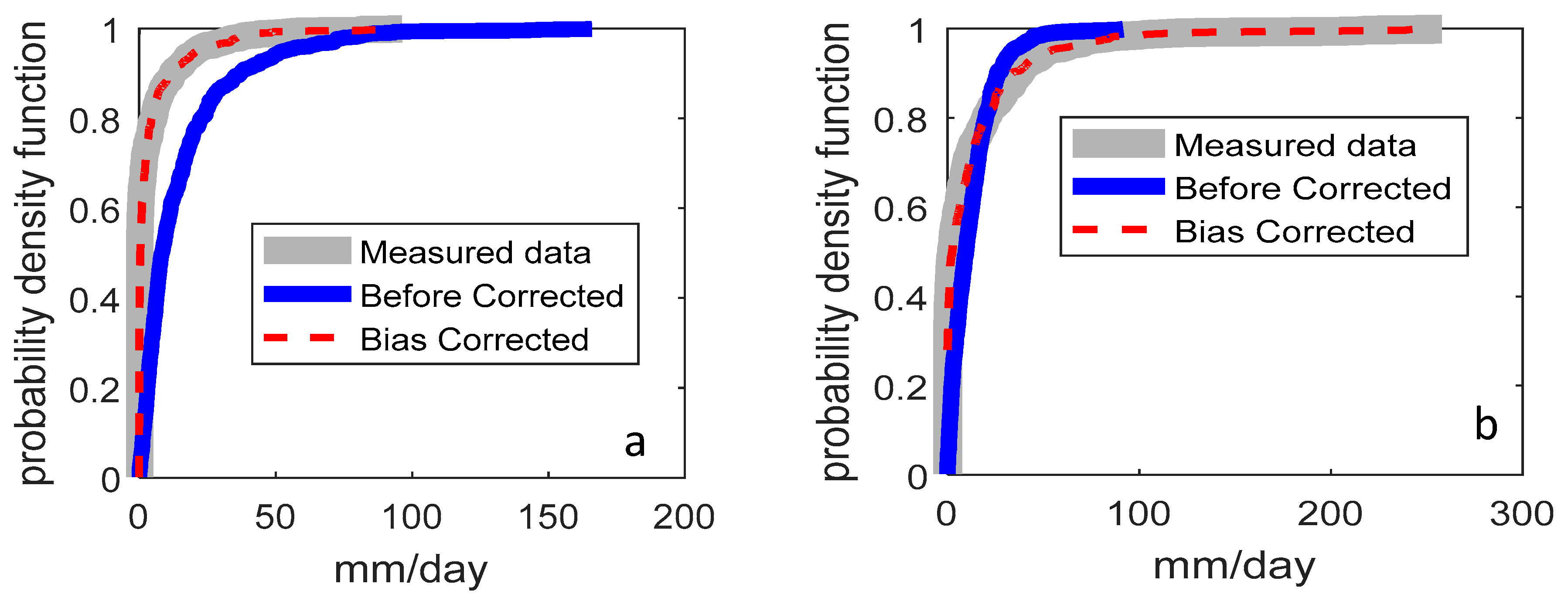
2.3.1. Bias Correction

Although the spatiotemporal resolution of dynamical downscaling models has considerably improved, regional climate models inevitably show systematic biases in their outputs. Therefore, a bias correction needs to be implemented to produce reliable climate simulations at high resolution scales of time and space. To date, there are lots of statistical downscaling approaches to downscale the data from GCMs to smaller scales [29,30,31,32]. The core of these methods is to build the statistical relationship between large-scale predictors and local-scale predictands (e.g., precipitation and temperature) derived from the observed data. Afterwards, these relationships are used to reproduce or project local climatic parameters from GCMs. Several methods of bias correction are introduced [2,24,33,34,35,36,37,38]. A list of the methods can be found in the Validating and Integrating Downscaling Methods for Climate Change Research [39]. Bias correction methods have usually proposed to downscale climate model outputs for the variables of precipitation and temperature. These methods range from simple approaches (e.g., linear scaling) to sophisticated approaches (e.g., quantile mapping) [40]. In this study, the method of two-steps adopted from Nguyen and Ines [24,34] is selected to correct the downscaled daily precipitation data aggregated from 3-hourly data at a station scale. The important point here is that the bias correction is successfully performed for the daily precipitation data, not only in the different regions of world, but in several regions of Vietnam in particular. The quality of extreme precipitation values is also improved using the bias correction as described in Nguyen [24]. Although several distributions (e.g., Gumbel, Log-normal, Generalized Extreme Value) are presented to discard the bias from the extremes directly [30,36], there is a need to make further investigations on these distributions under the precipitation regimes in Vietnam. It is emphasized that a consecutive series of daily precipitation from 2016 to 2099 is corrected in this study, but just only the above time slices are considered. The reason for this is that it is easier to compare the obtained results to other studies (e.g., the reports of MONRE of Vietnam). The principal idea of this method is to separate the precipitation processes into two parts: a model for the occurrence of wet days, and another model for precipitation amount on wet days. In the first part, the distribution of Weibull is fitted to the distribution of the observed precipitation days [41]. The method of least-square estimation for logarithmic transformation is applied to estimation of Weibull parameters for separate months. It is to be noted that only values greater than a threshold value of 0.1 mm/day identified for a wet day are taken into account in the station data time series for the period 1986–2005. The form of the Weibull distribution is the following:

$$\mathrm{F}\left(\mathrm{x}\right)=1-\exp \left[-{\left(\frac{\mathrm{x}}{\mathrm{b}}\right)}^{\mathrm{c}}\right]$$

(1)

where b is the scale parameter (b > 0); c is the shape parameter (c > 0).

On the basis of the relationship function between large-scale and local-scale values, the threshold value for large-scale daily precipitation series is calculated. This relationship function is described as:

$${\mathrm{x}}_{\mathrm{s}}={\mathrm{F}}_{\mathrm{s}}^{-1}\left({\mathrm{F}}_{\mathrm{o}}\left({\mathrm{x}}_{\mathrm{o}}\right)\right)$$

(2)

where x_o is local scale data; x_s is large scale data; ${\mathrm{F}}_{\mathrm{s}}^{-1}$ is the inverse function of F_s. The ${\mathrm{F}}_{\mathrm{s}}^{-1}$ function can be found by using the method of inverse transformation.

In the second part, the gamma distribution with two parameters is held in a series of data for the considered periods. This distribution is carried out separately for each calendar month with the large-scale amount of precipitation above the identified threshold. The parameters of this distribution are estimated using the method of maximum-likelihood. The form of the probability density function is expressed as:

$$\mathrm{f}\left(\mathrm{x}\right)=\frac{{\mathsf{\beta }}^{-\mathsf{\alpha }}{\mathrm{x}}^{\mathsf{\alpha }-1}}{\lceil \left(\mathsf{\alpha }\right)}\exp (\frac{-\mathrm{x}}{\mathsf{\beta }})\mathsf{\alpha },\mathsf{\beta },\mathrm{x}>0$$

(3)

where α and β denote the shape and scale parameter, respectively; x represents the daily precipitation amount; $\lceil \left(\mathsf{\alpha }\right)$ is the gamma function evaluated at α.

The amount of daily precipitation x (mm/day) in Equation (3) is defined as product of the mean intensity on wet days when precipitation exceeds 0.1 mm. This means that the days with an amount of precipitation less than 0.1 mm were excluded in the calculation.

Climate change signals of precipitation changes under RCP4.5 and RCP8.5 scenarios are calculated for each station on the basis of the following formulas:

$${\%\mathrm{P}}_{2030\mathrm{s}}=\left(\frac{{\mathrm{P}}_{2016-2035}-{\mathrm{P}}_{1986-2005}}{{\mathrm{P}}_{1986-2005}}\right)\times 100\%,$$

(4)

$${\%\mathrm{P}}_{2050\mathrm{s}}=\left(\frac{{\mathrm{P}}_{2046-2065}-{\mathrm{P}}_{1986-2005}}{{\mathrm{P}}_{1986-2005}}\right)\times 100\%,$$

(5)

$${\%\mathrm{P}}_{2090\mathrm{s}}=\left(\frac{{\mathrm{P}}_{2080-2099}-{\mathrm{P}}_{1986-2005}}{{\mathrm{P}}_{1986-2005}}\right)\times 100\%$$

(6)

where P is precipitation; subscript denotes the considered periods of baseline (1986–2005) and time slices of 2016–2035, 2046–2065 and 2080–2099 future under climate change scenarios of RCP4.5.

2.3.2. Intensity–Duration–Frequency (IDF) Curve

Typically, the development of the IDF curves involves three steps. Firstly, precipitation data for a number of precipitation durations (e.g., 1, 2, 6, 12, 24 h) is fitted by probability distribution function (PDF) or cumulative distribution function (CDF). Then, the maximum precipitation intensity for each time interval is related with the corresponding return period from the cumulative distribution function. Finally, from the known cumulative frequency and given duration, the maximum precipitation intensity can be determined using an appropriately fitted theoretical distribution function (e.g., Generalized Extreme Value Distribution (GEV), Gumbel, Pearson Type III). Commonly, the probability distribution of Gumbel (Extreme Value Type I) is applied to analyze the extreme precipitation statistics, and has been selected in this study. A brief description of the probability distribution is represented below.

Gumbel distribution has a cumulative distribution function:

$$\mathrm{F}\left(\mathrm{x}\right)=\left(\frac{\mathrm{T}-1}{\mathrm{T}}\right)={\mathrm{e}}^{-{\mathrm{e}}^{-\frac{\left(\mathrm{x}-\mathrm{u}\right)}{\mathsf{\alpha }}}}$$

(7)

where T is the return period. The parameters of the Type I function α and u are expressed by the following equations:

$$\mathsf{\alpha }=\frac{\sqrt{6}{\mathrm{S}}_{\mathrm{x}}}{\mathsf{\pi }},$$

(8)

$$\mathrm{u}=\overline{\mathrm{x}}-0.5772\mathsf{\alpha }$$

(9)

where ${\mathrm{S}}_{\mathrm{x}}$ and $\overline{\mathrm{x}}$ are the standard deviation and mean of the maximum annual precipitation dataset.

In order to develop the IDF curves for a wide range of sub-daily scales (e.g., 1, 3 h) from daily data, the correlation coefficients on precipitation heights is made and defined for 15 homogeneous zones in which the hydrologic regime of intense events is similar [42]. In this study, the same procedure is applied, considering as first attempt values the coefficients defined [42] and validating them by a specific analysis carried on the two stations (i.e., Danang and Tramy) where hourly data is available during 1990–2015. In these stations maximum annual precipitation heights for 1, 3, 6, 12, 24, 48 and 72 h are computed and confronted with maximum heights for 1, 2 and 3 days at the same stations. As the size of most sub-basins is relatively big, concentration times are mostly in the range 12–36 h, so durations longer than 24 h are included in IDF computation in order to improve the critical precipitation estimation in the range of interest. The results obtained in terms of correlation factors between daily and hourly precipitation are quite consistent and similar between the two considered stations. Thus, a simple mean of the coefficients evaluated for the two stations is taken as reference for the estimations of IDF curves in all VG-TB basin. As presented in

Table 2. Correlation coefficient between daily and hourly maximum precipitation heights.

Duration	1 h	3 h	6 h	12 h	24 h	48 h	72 h
Danang station	0.756	0.768	0.881	0.990	1.084	1.063	1.034
Tramy station	0.706	0.808	0.983	1.042	1.087	1.056	1.039
Mean value	0.731	0.788	0.932	1.016	1.086	1.059	1.037
	to be applied to “references” coefficient				to be applied directly on data

, these coefficients are intended as correction of the coefficients defined for durations from 1 to 12 h and as correlation coefficients to be applied directly on daily data for durations from 24 to 72 h [42].

After this calibration of correlation coefficients, it is possible to estimate maximum annual values of precipitation heights for given hourly durations for all stations with daily data and evaluate IDF curves with statistical analysis of obtained series. Daily data are generally available for the period 1977–2016 on all stations. For easier use in the following phases, IDF curves are expressed with reference to precipitation height and not intensity, using the following monomial formula (power function):

h = a·tⁿ; i = a·n·tⁿ⁻¹

(10)

where h is the depth of precipitation (mm) for the duration t; i = h/t is the precipitation intensity; a, n are parameters to estimate from the data series.

In brief, the process of construction the future IDF curves involves the following steps: (1) bias correction of the regional precipitation data for different periods of baseline and future using the measured data under different scenarios of climate change; (2) develop a method based on the correlation equation from measured stations to calculate the sub-daily scales (e.g., 1, 3, 6 h); (3) obtain the annual maximum series of precipitation intensity for each considered duration; (4) apply the Gumbel distribution to find precipitation depths for different return periods; (5) repeat steps 3 and 4 for each duration; and (6) repeat steps 1 to 5 for different periods of baseline and future. It is specifically emphasized that an assumption of the correlation coefficients between the hourly and daily precipitation values is no change in the future and therefore there will be no changes in the temporal distribution of precipitation. This assumption is investigated and described in Christensen & Christensen [43], Buonomo et al. [44] and Rodríguez et al. [45].

3. Results and Discussions

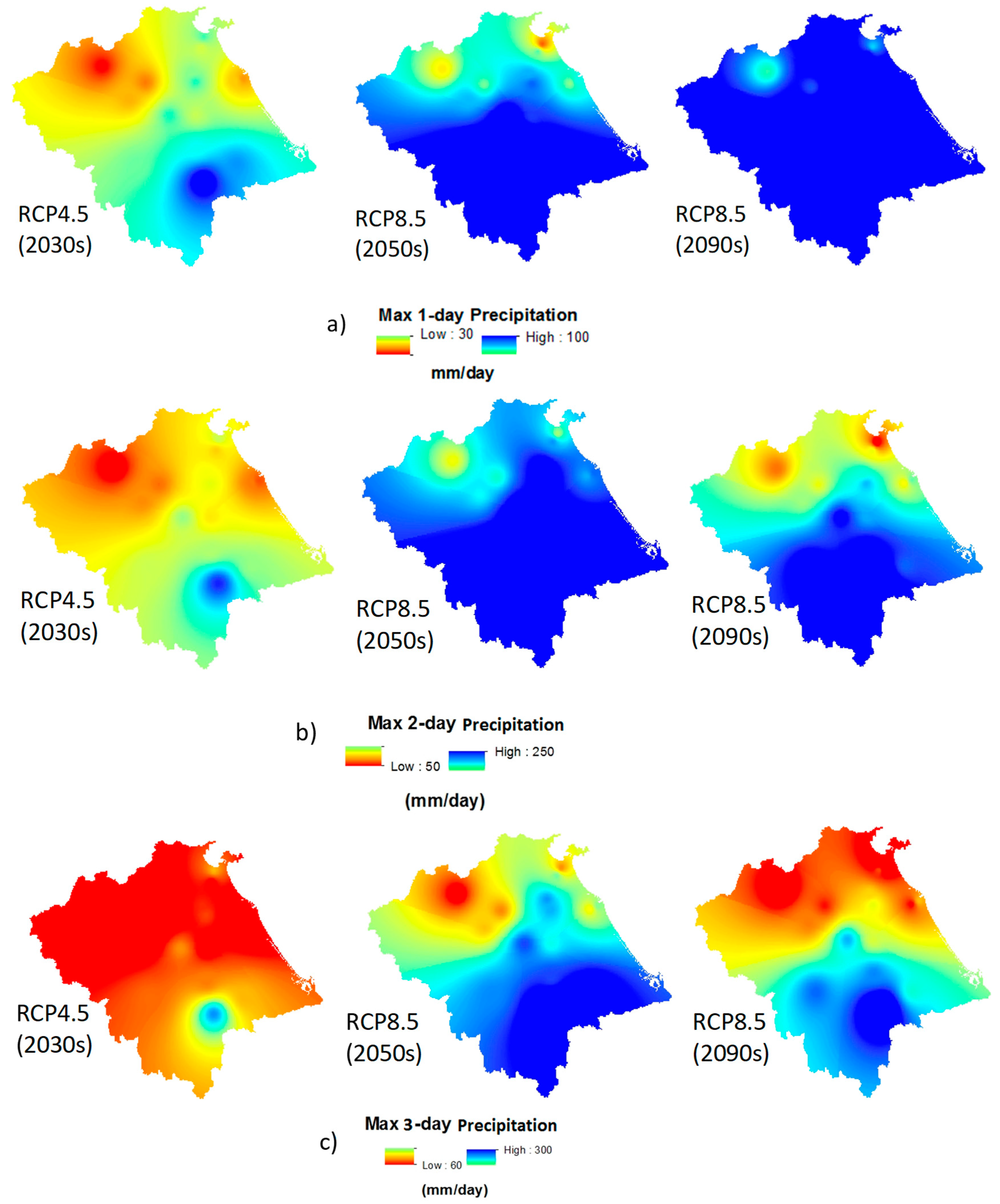
3.1. Projected Precipitation Changes

As is illustrated over the VG-TB basin, it can be concluded that the precipitation simulated by RCM/ICHEC is much higher than the observation precipitation, especially in the area of Tramy station (more than 230 mm/month) (Figure 2). The bias tends to enlarge towards the south of the basin. This likely deal with the complex orographic effects of mountain peaks. Meanwhile, along the east and northeast of the basin, there is a decrease in the bias of reproduced precipitation against the observation precipitation in comparison with other areas of basin. The bias ranges from about 35 mm/month to over100 mm/month. Additionally, a positive bias of the reproduced precipitation minus the observation data is found over land mask in case RCM/MPI; however, it is lower than reproduced precipitation in case RCM/ICHE. More importantly, a negative bias is mostly depicted over the whole VG-TB basin when the precipitation reproduced by RCM/IPSL. Indeed, the performance of regional climate models forced by different global climate models are affected by a wide range of factors (e.g., initial conditions, cloud parameterize schemes). This mainly causes the unexpected precipitation simulations. To eliminate uncertainty, however, an ensemble of RCM/ICHEC, RCM/MPI and RCM/IPSL is analyzed and shown. Furthermore, a bias correction is applied. Although this correction method is carried out for all stations in the VG-TB basin, in this part of the study, the results of the corrected daily precipitation are shown in Figure 3 for Tramy and Danang as typical examples.

Figure 3 depicts that the precipitation simulations fit better to the measured precipitation with bias correction than without in September, October and November for both Tramy and Danang stations. In May and June, the corrected precipitation amount fits well to the observed precipitation at Tramy and Danang station. The monthly biases fall down to 300 mm/month from 450 mm/month in May for Tramy station (Figure 3a) and to nearly 50 mm/month from over 300 mm/month in May and June for Danang station (Figure 3b). It is noteworthy that there is a sharp augment in the reproduced precipitation from about 450 mm/month climbing over 1050 mm/month during October and September for Tramy station (Figure 3a). It is seen that a precipitation amount of about 150 mm/month is additionally filled out in September and October for Danang station after bias correction (Figure 3b).

The probability density function graph shows the effects of bias correction on the distribution of precipitation simulations in January and in August for Tramy station as a typical example. It can be seen from the graph that the extreme and drizzle values of precipitation simulations in August (Figure 4b) and January (Figure 4a) are eliminated, respectively.

The box plot of the day of year of precipitation before and after bias correction against measured data shows in Figure 5. It is observed that results for the median for all stations with bias correction are much better than without. The values of extreme differences with bias correction and without are also improved (Figure 5). This is to be expected, because sophisticated interactions of weather patterns and orographic that cause extreme events during the rainy season over this basin (e.g., interactions of the Intertropical Convergence Zone and tropical cyclones in central Vietnam). Furthermore, the foundation and development of convective processes are vital for weather patterns in the tropical monsoon region, but are nearly unpredictable.

Table 3. Projected precipitation changes under RCP4.5 and RCP8.5 scenarios in comparison with baseline period for 15 stations over the VG-TB basin (%).

Stations	Under RCP4.5 Scenario	Under RCP8.5 Scenario
	2030s	2050s	2090s
Ainghia	18.8	28.7	20.8
Camle	29.3	26.5	31.6
Caulau	11.3	18.7	18.1
Giaothuy	18.1	19.6	19.8
Hien	13.3	19.3	16.5
Hiepduc	14.3	21.4	20.0
Hoian	19.8	26.2	23.6
Hoikhanh	15.3	21.9	17.7
Khamduc	11.4	17.1	18.7
Nongson	15.8	22.5	19.1
Queson	15.9	22.0	19.3
Thanhmy	14.3	20.2	16.9
Tienphuoc	14.2	23.3	20.6
Danang	14.0	24.2	19.9
Tramy	16.6	27.2	26.8

depicts information on the change signals of projected precipitation. Under the RCP4.5 scenario, projected precipitation changes amount to over 16% and 14% for Tramy and Danang station during the 2030s, respectively. Meanwhile, an increase in the projected precipitation to over 24% and 27% is illustrated during the 2050s under RCP8.5 for Danang and Tramy station, respectively. On a provincial scale, a negligible difference of projected precipitation changes is found in comparison with the report of MONRE (2016). For example, according to the report of MONRE (2016), the projected precipitation change is expected to increase by up to 16.2% and 22.0% in case of RCP4.5 and RCP8.5 for Danang province.

Under RCP4.5 Scenario during the 2030s, the highest increase in the projected precipitation changes was calculated for Camle (29.3%), whereas the lowest value was for Caulau (11.3%). It is noteworthy that location of these stations is quite close, but the projected precipitation is quite different. The reason for this is that precipitation strongly patterns in time and space, especially in central Vietnam. Precipitation regimes over this region are significantly controlled by the combination of a steep topography, tropical cyclones, monsoon systems and tropical disturbances in the Intertropical Convergence Zone. Importantly, in comparison with the 2050s, there is a small decrease in the projected precipitation during the 2090s under RCP8.5 scenarios for most considered stations. Namely, the percentage of precipitation change falls down to 20.8% (2090s) from 28.7% (2050s). As shown in Table 3, under the RCP8.5 scenario, three out of fifteen stations are expected to increase from 26.5%, 19.6% and 17.1% in 2050s and to 31.6%, 19.8% and 18.7% in 2090s for Camle, Giaothuy and Khamduc stations, respectively.

Under the considered climate change scenarios, the projected changes of a maximum of 1, 2 and 3 days precipitation are calculated. A significant increase in a maximum of 1-day precipitation is expected for the south of VG-TB basin (over 100 mm/day), especially in the 2090s (Figure 6). Contrary to this, in the north of VG-TB basin there is a light increase in maximum 1-day precipitation in the year 2030s under RCP4.5 scenario (about 30 mm/day) (Figure 6). In the south of VG-TB basin, the projected changes of a maximum of 2- and 3-days precipitation are expected to increase by about 300 mm/day under RCP8.5 scenario in the year 2090s.The projected precipitation over the north of VG-TB is lower than that over the south of VG-TB in both of RCP8.5 in the year 2050s and 2090s. It can be seen that an increase of about 30–300 mm/day in the projected changes of 1-, 2-, and 3-days precipitation is expected under the considered scenarios. All these are considered to project the IDF curves changes under climate change conditions.

In general, with the purpose of adjusting the statistics of climate simulations to better match observed statistics over present-day reference periods, bias correction gives added value with downscaled steps. It is noteworthy that the selection of regional climate models or global climate models is very important because the chosen climate model produces skillful input for a bias correction. Moreover, the features of physical processes from dynamical climate models are involved if the finest resolution of climate model is applied. The major sources of uncertainty in this study come from: (i) selection of parameterization schemes and resolution in the dynamical downscaling models; (ii) greenhouse gas concentration scenarios; and (iii) technique of bias correction.

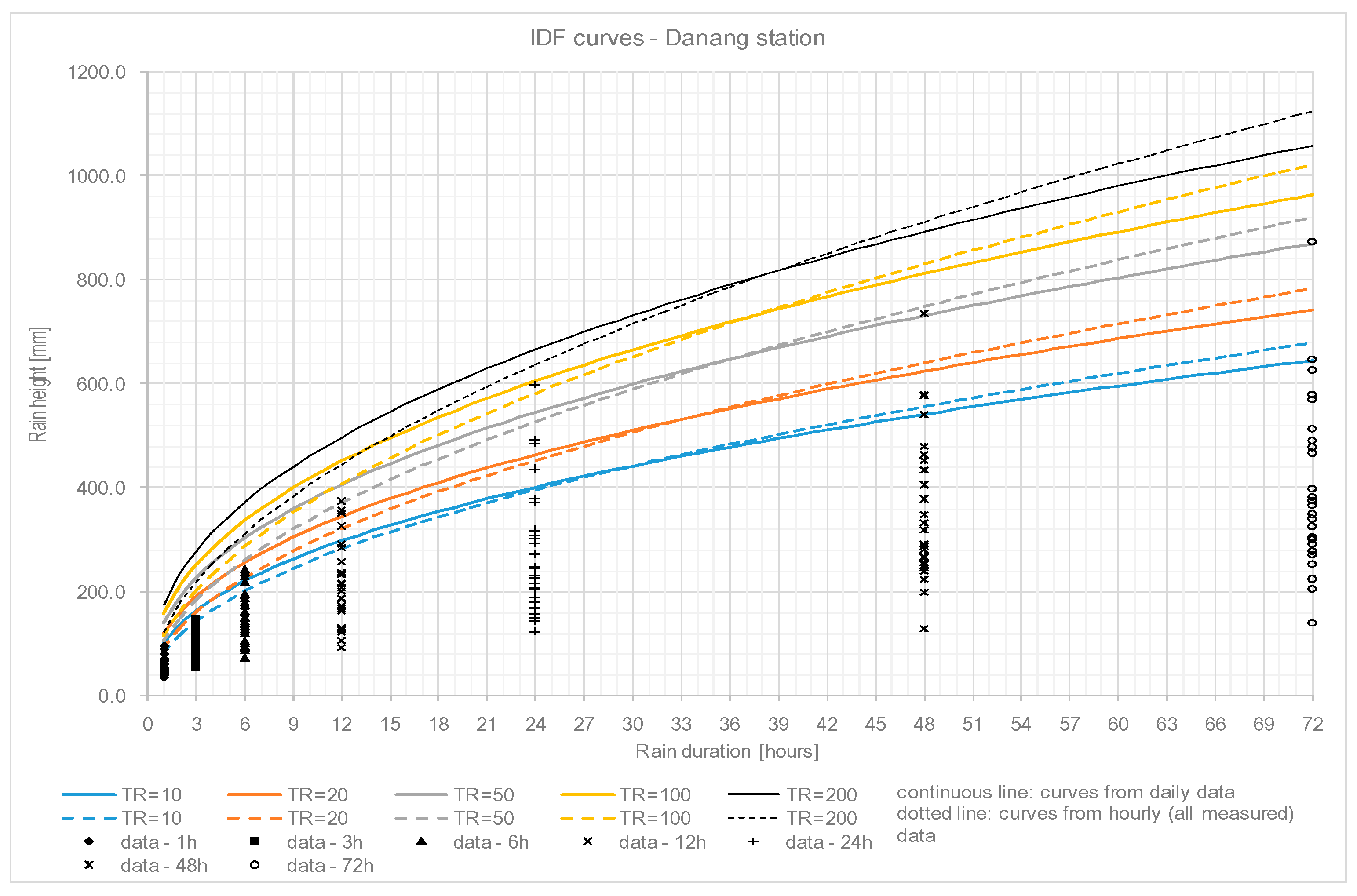
3.2. Construction of the IDF Curves

Using the hourly and daily precipitation data from 1990–2016 at Tramy and Danang stations, the IDF curves are evaluated by fitting a Gumbel probability distribution to the data series. This distribution, also known as the General Extreme Values distribution (GEV)–type I, is the asymptotic form of maximum values of all distribution probability with exponential decline (“tail” of the curve), including Gaussian, Lognormal, Pearson type III (which is a gamma distribution), etc. This distribution is thus very general and flexible and easy to apply as the parameters estimation using minimum-square method can be expressed with an explicit formula. Figure 7 and Figure 8 show the differences between IDF curves evaluated from hourly data series and with the estimation procedure based on daily data previously described.

Curves from daily data tend to be more conservative for short and medium precipitation durations and less conservative for very long durations. Around 36 h duration the values from the two kinds of curves are very similar. Thus, considering that concentration times for defined sub-basins in VG-TB are mostly in the range 12–36 h, the choice to rely on daily data is consistent, as it is not underestimating the risk levels (resulting precipitation heights will be the same or slightly increased than the ones that can be obtained by hourly data analysis–available only in very few stations). IDF curves are computed with this procedure for the case of different return periods (i.e., 10, 20, 50, 100 and 200 years) for each available station in the basin area. Results are presented in

Table 4. Parameters a and n for various return periods (years) for the gauging stations in VG-TB basin.

Parameter	a (10 years)	a (20 years)	a (50 years)	a (100 years)	a (200 years)	n (10 years)	n (20 years)	n (50 years)	n (100 years)	n (200 years)
Ainghia	71.78	81.83	94.84	104.59	114.30	0.53	0.54	0.54	0.54	0.54
Camle	80.51	94.55	112.75	126.39	139.98	0.50	0.49	0.49	0.49	0.49
Caulau	62.29	71.38	83.15	91.97	100.76	0.54	0.55	0.55	0.55	0.55
Giaothuy	68.30	77.59	89.62	98.64	107.63	0.54	0.54	0.54	0.54	0.54
Hien	65.01	76.08	90.42	101.17	111.89	0.53	0.52	0.52	0.52	0.52
Hiepduc	78.55	88.82	102.12	112.09	122.03	0.55	0.56	0.56	0.56	0.56
Hoian	73.40	86.37	103.16	115.75	128.29	0.52	0.52	0.52	0.52	0.52
Hoikhanh	59.93	69.00	80.74	89.54	98.30	0.55	0.55	0.56	0.56	0.56
Khamduc	72.60	82.99	96.43	106.51	116.55	0.55	0.54	0.54	0.54	0.54
Nongson	65.20	72.21	81.30	88.12	94.92	0.55	0.56	0.56	0.56	0.57
Queson	69.19	79.13	92.00	101.64	111.25	0.53	0.53	0.53	0.53	0.53
Thanhmy	71.78	81.83	94.84	104.59	114.30	0.53	0.54	0.54	0.54	0.54
Tienphuoc	80.56	91.06	104.65	114.83	124.97	0.54	0.54	0.54	0.54	0.54
Danang	77.84	90.97	107.96	120.70	133.39	0.51	0.51	0.51	0.50	0.50
Tramy	81.58	92.13	105.80	116.04	126.24	0.55	0.55	0.55	0.54	0.54

.

The selection of return periods are of practical relevance for design and operation of reservoirs, damps, dikes and drainage systems. Gumbel distribution was used to produce the IDF curves for the periods of 1986–2005, 2016–2035, 2046–2065 and 2080–2099 future under climate change scenarios. Analysis of median of projected precipitation intensity changes for durations from 1 to 72 h with return periods of 10-, 20-, 50-, 100- and 200-years for VG-TB basin depicted in Figure 9. Over the basin, generally, there is a slight increase in projected precipitation intensity changes with return periods of from 10 to 200 years for both the scenarios of RCP4.5 and RCP8.5. Under the scenario of RCP4.5 (2030s), the precipitation intensity changes are expected to increase between about 90% and 110% with a return period of 10-, 200-years, respectively. It is seen that the lowest and highest values of precipitation intensity changes are projected for a return period of 10 years (nearly 150%) and of 200 years (nearly 200%) under scenario of RCP8.5 (2090s). An increase in projected precipitation intensity changes is expected to reach 200% with a return period of about 200 years from about 160% with a return period of 10 years under scenario of RCP8.5 (2050s). This is consistent to the previous analysis of projected maximum 1 day precipitation changes.

4. Conclusions

This study presents the projected changes of precipitation events and constructs the intensity–duration–frequency curves for short durations of precipitation under the context of global warming on the basis of the combination of spatial dynamical downscaling, bias correction and terms of correlation factors. The work is implemented for the VuGia-ThuBon basin located in central Vietnam where the patterns of climate regime are complex.

The major findings of the present study can be exposed an impulse of the precipitation simulations after bias correction. With bias correction, an ensemble of precipitation simulations run from the regional climate model RegCM4 driven by three global models—MPI-ESM-MR, IPSL-CM5A-LR and ICHEC-EC-EARTH—at the finest resolution of a hydrostatic climate model were well fitted to the measured precipitation. Importantly, the level of accuracy precipitation simulations for extreme and drizzle events were also enhanced. Under the scenarios of RCP4.5 and RCP8.5, the possible precipitation changes were projected to increase by about 10 to 30% for all stations over the VuGia-ThuBon basin. To be more specific, a clear increase in projected precipitation changes is expected to range from 11.3% and 29.3% under the RCP4.5 scenario during the period 2030s. Under the RCP8.5 scenario, the projected precipitation changes are expected to increase between 17.1% and 28.7%, and 16.5% and 31.6% for the period 2050s and 2090s, respectively.

The precipitation IDF curves are well produced using terms of correlation factors before constructing these curves for corrected climate simulations. The present and future IDF curves are completely built for short durations of from 1 to 72 h with return periods of 10-, 20-, 50-, 100- and 200-years. There is an increased tendency of projected precipitation intensity changes between climate change scenarios of RCP4.5 (2030s), RCP8.5 (2050s) and RCP8.5 (2090s) with the same expected of return period. Compared to other considered scenarios, under the scenario of RCP4.5 (2050s), it is documented the highest values of projected precipitation intensity changes with return periods of 10 years (about 160%), 20 years (175%), 50 years (188%), 100 years (195% and 200 years (about 200%). With all considered return periods, in comparison with the baseline period (1986–2005) the intensities of extreme precipitation events are about 90% and 110% under the scenario of RCP4.5 (2030s), and nearly 150% and 200% under scenario of RCP8.5 (2090s). All these imply that intense precipitation events are likely to occur more frequently in the future under the context of global warming.

References

1. Solomon, S.; Qin, D.; Manning, M.; Averyt, K.; Marquis, M. Climate Change 2007—The Physical Science Basis: Working Group I Contribution to the Fourth Assessment Report of the IPCC; Cambridge University Press: Cambridge, UK, 2007; Volume 4. [Google Scholar]
2. Myhre, G.; Shindell, D.; Bréon, F.M.; Collins, W.; Fuglestvedt, J.; Huang, J.; Koch, D.; Lamarque, J.F.; Lee, D.; Mendoza, B.; et al. Climate Change 2013: The Physical Science Basis. Contribution of Working Group I to the Fifth Assessment Report of the Intergovernmental Panel on Climate Change; Cambridge University Press: Cambridge, UK; New York, NY, USA, 2013; p. 1535. [Google Scholar]
3. Amirabadizadeh, M.; Huang, Y.F.; Lee, T.S. Recent trends in temperature and precipitation in the Langat River basin, Malaysia. Adv. Meteorol. 2015, 2015, 579437. [Google Scholar] [CrossRef]
4. Donat, M.G.; Peterson, T.C.; Brunet, M.; King, A.D.; Almazroui, M.; Kolli, R.K.; Boucherf, D.; Al-Mulla, A.Y.; Nour, A.Y.; Aly, A.A.; et al. Changes in extreme temperature and precipitation in the Arab region: Long-term trends and variability related to ENSO and NAO. Int. J. Climatol. 2014, 34, 581–592. [Google Scholar] [CrossRef]
5. Kwarteng, A.Y.; Dorvlo, A.S.; Kumar, G.T.V. Analysis of a 27-year rainfall data (1977–2003) in the Sultanate of Oman. Int. J. Climatol. 2009, 29, 605–617. [Google Scholar] [CrossRef]
6. Lovino, M.; García, N.O.; Baethgen, W. Spatiotemporal analysis of extreme precipitation events in the Northeast region of Argentina (NEA). J. Hydrol. Reg. Stud. 2014, 2, 140–158. [Google Scholar] [CrossRef]
7. Dash, S.K.; Jenamani, R.K.; Kalsi, S.R.; Panda, S.K. Some evidence of climate change in twentieth-century India. Clim. Chang. 2007, 85, 299–321. [Google Scholar] [CrossRef]
8. Shrestha, A.B.; Wake, C.P.; Dibb, J.E.; Mayewski, P.A. Precipitation fluctuations in the Nepal Himalaya and its vicinity and relationship with some large scale climatological parameters. Int. J. Climatol. 2000, 20, 317–327. [Google Scholar] [CrossRef] [Green Version]
9. Liu, B.; Xu, M.; Henderson, M.; Qi, Y. Observed trends of precipitation amount, frequency, and intensity in China, 1960–2000. J. Geophys. Res. Atmos. 2005, 110. [Google Scholar] [CrossRef] [Green Version]
10. Limsakul, A.; Singhruck, P. Long-term trends and variability of total and extreme precipitation in Thailand. Atmos. Res. 2016, 169, 301–317. [Google Scholar] [CrossRef]
11. Phan, V.T. Non-Parametric Test for Trend of Change of Some Climate Variables During the Period 1961–2007; Vietnam National University: Hanoi, Vietnam, 2012; Volume 28, pp. 129–135. (In Vietnamese) [Google Scholar]
12. Nguyen, T.T. Fitting a Probability Distribution to Extreme Precipitation for a Limited Mountain Area in Vietnam. J. Geosci. Environ. Prot. 2017, 5, 92. [Google Scholar]
13. Akan, A.O.; Houghtalen, R.J. Urban Hydrology, Hydraulics, and Stormwater Quality: Engineering Applications and Computer Modeling; John Wiley & Sons: Hoboken, NJ, USA, 2003. [Google Scholar]
14. Koutsoyiannis, D.; Kozonis, D.; Manetas, A. A mathematical framework for studying rainfall intensity-duration-frequency relationships. J. Hydrol. 1998, 206, 118–135. [Google Scholar] [CrossRef]
15. Sivapalan, M.; Blöschl, G. Transformation of point rainfall to areal rainfall: Intensity-duration-frequency curves. J. Hydrol. 1998, 204, 150–167. [Google Scholar] [CrossRef]
16. Coulibaly, P.; Shi, X. Identification of the Effect of Climate Change on Future Design Standards of Drainage Infrastructure in Ontario; Report Prepared by McMaster University with Funding from the Ministry of Transportation of Ontario; McMaster University: Hamilton, ON, Canada, 2005. [Google Scholar]
17. KIm, T.W.; Wi, S.; Valdés-Pineda, R.; Valdés, J.B. Future Projection of Design Storms Using a GCM-Informed Weather Generator. In AGU Fall Meeting Abstracts; American Geophysical Union: Washington, DC, USA, 2017. [Google Scholar]
18. Mailhot, A.; Duchesne, S.; Caya, D.; Talbot, G. Assessment of future change in intensity–duration–frequency (IDF) curves for Southern Quebec using the Canadian Regional Climate Model (CRCM). J. Hydrol. 2007, 347, 197–210. [Google Scholar] [CrossRef]
19. Clarke, L.; Edmonds, J.; Jacoby, H.; Pitcher, H.; Reilly, J.; Richels, R. Scenarios of Greenhouse Gas Emissions and Atmospheric Concentrations; US Department of Energy Publications: Washington, DC, USA, 2007; p. 6. [Google Scholar]
20. Wise, M.; Calvin, K.; Thomson, A.; Clarke, L.; Bond-Lamberty, B.; Sands, R.; Smith, S.J.; Janetos, A.; Edmonds, J. Implications of limiting CO2 concentrations for land use and energy. Science 2009, 324, 1183–1186. [Google Scholar] [CrossRef] [PubMed]
21. Riahi, K.; Rao, S.; Krey, V.; Cho, C.; Chirkov, V.; Fischer, G.; Kindermann, G.; Nakicenovic, N.; Rafaj, P. RCP 8.5—A scenario of comparatively high greenhouse gas emissions. Clim. Chang. 2011, 109, 33. [Google Scholar] [CrossRef]
22. Yatagai, A.; Kamiguchi, K.; Arakawa, O.; Hamada, A.; Yasutomi, N.; Kitoh, A. APHRODITE: Constructing a long-term daily gridded precipitation dataset for Asia based on a dense network of rain gauges. Bull. Am. Meteorol. Soc. 2012, 93, 1401–1415. [Google Scholar] [CrossRef]
23. Harris, I.P.; Jones, P.D.; Osborn, T.J.; Lister, D.H. Updated high-resolution grids of monthly climatic observations–the CRU TS3. 10 Dataset. Int. J. Climatol. 2014, 34, 623–642. [Google Scholar] [CrossRef] [Green Version]
24. Nguyen, T.T. Improved Downscaling of Meteorological Data for Hydrological Modeling in the Tropics Under Climate Change. Ph.D. Thesis, Technische Universität Carolo-Wilhelmina zu Braunschweig, Braunschweig, Germany, 2016. [Google Scholar]
25. Giorgetta, M.A.; Jungclaus, J.; Reick, C.H.; Legutke, S.; Bader, J.; Böttinger, M.; Brovkin, V.; Crueger, T.; Esch, M.; Fieg, K.; et al. Climate and carbon cycle changes from 1850 to 2100 in MPI-ESM simulations for the Coupled Model Intercomparison Project phase 5. J. Adv. Model. Earth Syst. 2013, 5, 572–597. [Google Scholar] [CrossRef] [Green Version]
26. Stevens, B.; Giorgetta, M.; Esch, M.; Mauritsen, T.; Crueger, T.; Rast, S.; Salzmann, M.; Schmidt, H.; Bader, J.; Block, K.; et al. Atmospheric component of the MPI-M Earth System Model: ECHAM6. J. Adv. Model. Earth Syst. 2013, 5, 146–172. [Google Scholar] [CrossRef] [Green Version]
27. Dufresne, J.L.; Foujols, M.A.; Denvil, S.; Caubel, A.; Marti, O.; Aumont, O.; Balkanski, Y.; Bekki, S.; Bellenger, H.; Benshila, R.; et al. Climate change projections using the IPSL-CM5 Earth System Model: From CMIP3 to CMIP5. Clim. Dyn. 2013, 40, 2123–2165. [Google Scholar] [CrossRef] [Green Version]
28. Hazeleger, W.; Wang, X.; Severijns, C.; Ştefănescu, S.; Bintanja, R.; Sterl, A.; Wyser, K.; Semmler, T.; Yang, S.; Van den Hurk, B.; et al. EC-Earth V2.2: Description and validation of a new seamless earth system prediction model. Clim. Dyn. 2012, 39, 2611–2629. [Google Scholar] [CrossRef]
29. Hewitson, B.; Crane, R. Climate downscaling: Techniques and application. Clim. Res. 1996, 7, 85–95. [Google Scholar] [CrossRef]
30. Maraun, D.; Wetterhall, F.; Ireson, A.M.; Chandler, R.E.; Kendon, E.J.; Widmann, M.; Brienen, S.; Rust, H.W.; Sauter, T.; Themeßl, M.; et al. Precipitation downscaling under climate change: Recent developments to bridge the gap between dynamical models and the end user. Rev. Geophys. 2010, 48. [Google Scholar] [CrossRef] [Green Version]
31. Wilby, R.L.; Charles, S.P.; Zorita, E.; Timbal, B.; Whetton, P.; Mearns, L.O. Guidelines for Use of Climate Scenarios Developed from Statistical Downscaling Methods. In Supporting Material of the Intergovernmental Panel on Climate Change (IPCC); Prepared on Behalf of Task Group on Data and Scenario Support for Impacts and Climate Analysis (TGICA); 2004; 27p, Available online: www.ipcc-data.org (accessed on 10 July 2018).
32. Wilby, R.L.; Wigley, T.M.; Conway, D.; Jones, P.D.; Hewitson, B.C.; Main, J.; Wilks, D.S. Statistical downscaling of general circulation model output: A comparison of methods. Water Resour. Res. 1998, 34, 2995–3008. [Google Scholar] [CrossRef] [Green Version]
33. Dosio, A.; Paruolo, P.; Rojas, R. Bias correction of the ENSEMBLES high resolution climate change projections for use by impact models: Analysis of the climate change signal. J. Geophys. Res. Atmos. 2012, 117. [Google Scholar] [CrossRef] [Green Version]
34. Ines, A.V.; Hansen, J.W. Bias correction of daily GCM rainfall for crop simulation studies. Agric. For. Meteorol. 2006, 138, 44–53. [Google Scholar] [CrossRef]
35. Lafon, T.; Dadson, S.; Buys, G.; Prudhomme, C. Bias correction of daily precipitation simulated by a regional climate model: A comparison of methods. Int. J. Climatol. 2013, 33, 1367–1381. [Google Scholar] [CrossRef] [Green Version]
36. Maraun, D. Bias correcting climate change simulations—A critical review. Curr. Clim. Chang. Rep. 2016, 2, 211–220. [Google Scholar] [CrossRef]
37. Piani, C.; Haerter, J.; Coppola, E. Statistical bias correction for daily precipitation in regional climate models over Europe. Theor. Appl. Climatol. 2010, 99, 187–192. [Google Scholar] [CrossRef]
38. Piani, C.; Weedon, G.P.; Best, M.; Gomes, S.M.; Viterbo, P.; Hagemann, S.; Haerter, J.O. Statistical bias correction of global simulated daily precipitation and temperature for the application of hydrological models. J. Hydrol. 2010, 395, 199–215. [Google Scholar] [CrossRef]
39. Maraun, D. VALUE–Validating and Integrating Downscaling Methods for Climate Change Studies; European Science Foundation: Brussels, Belgium, 2011. [Google Scholar]
40. Teutschbein, C.; Seibert, J. Bias correction of regional climate model simulations for hydrological climate-change impact studies: Review and evaluation of different methods. J. Hydrol. 2012, 456, 12–29. [Google Scholar] [CrossRef]
41. Weibull, W. A statistical distribution function of wide applicability. J. Appl. Mech. 1951, 18, 293–297. [Google Scholar]
42. United Nations Educational, Scientific and Cultural Organization (UNESCO). Asian Pacific FRIEND—Intensity Frequency Duration and Flood Frequencies Determination Meeting—Flow regimes from International Experimental and Network Data; UNESCO: Paris, France, 2005. [Google Scholar]
43. Buonomo, E.; Jones, R.; Huntingford, C.; Hannaford, J. On the robustness of changes in extreme precipitation over Europe from two high resolution climate change simulations. Q. J. R. Meteorol. Soc. 2007, 133, 65–81. [Google Scholar] [CrossRef] [Green Version]
44. Christensen, J.H.; Christensen, O.B. Climate modelling: Severe summertime flooding in Europe. Nature 2003, 421, 805. [Google Scholar] [CrossRef] [PubMed]
45. Rodríguez, R.; Navarro, X.; Casas, M.C.; Ribalaygua, J.; Russo, B.; Pouget, L.; Redaño, A. Influence of climate change on IDF curves for the metropolitan area of Barcelona (Spain). Int. J. Climatol. 2014, 34, 643–654. [Google Scholar] [CrossRef] [Green Version]
Figure 1. Network of hydro-meteorological stations at VG-TB basin.
Hydrology 05 00033 g001
Figure 2. Spatial distribution bias of the precipitation simulations minus observations during 1986–2005 (mm/month).
Hydrology 05 00033 g002
Figure 3. Before and after corrected precipitation in comparison with measured data for (a) Tramy station and (b) Danang station.
Hydrology 05 00033 g003
Figure 4. Before and after corrected precipitation in comparison with measured data for Tramy station in January (a) and August (b).
Hydrology 05 00033 g004
Figure 5. Box plot of the day of year of precipitation before (top) and after (bottom) bias correction minus measured data for 15 stations in VG-TB basin during 1986–2005 (mm/day).
Hydrology 05 00033 g005
Figure 6. Projected changes of maximum 1- (a), 2- (b) and 3- (c) days under climate change scenarios.
Hydrology 05 00033 g006
Figure 7. Confrontation between curves obtained from hourly and daily data at Danang station.
Hydrology 05 00033 g007
Figure 8. Confrontation between curves obtained from hourly and daily data at Tramy station.
Hydrology 05 00033 g008
Figure 9. Median of projected precipitation intensity changes for durations from 1 to 72 h with different return periods (TR) under scenarios of RCP4.5 (2030s), RCP8.5 (2050s) and RCP8.5 (2090s).
Hydrology 05 00033 g009