Changes in Temperature and Rainfall as a Result of Local Climate Change in Pasadena, California
Abstract
:1. Introduction
2. Pasadena and Its Environment
3. Study Design
3.1. Hypothesis
3.2. Study Design
- Organization: There are three parts to this study. The first two parts involves air temperatures in the City of Pasadena for evidence of local climate change. The third part examined changes in rainfall in Pasadena.
- Periods:
- The Study Period covered the 1880s to 2016 depending on the location.
- The Base Period covered the years 1910–2000 and was used a baseline for changes in temperature.
- The Control Period covered all years prior to 1950.
- The Test Period covered 1950 and all subsequent years.
- These Control and Test Periods were selected to divide the rainfall data into two equal halves and the air temperatures into two approximately equal populations.
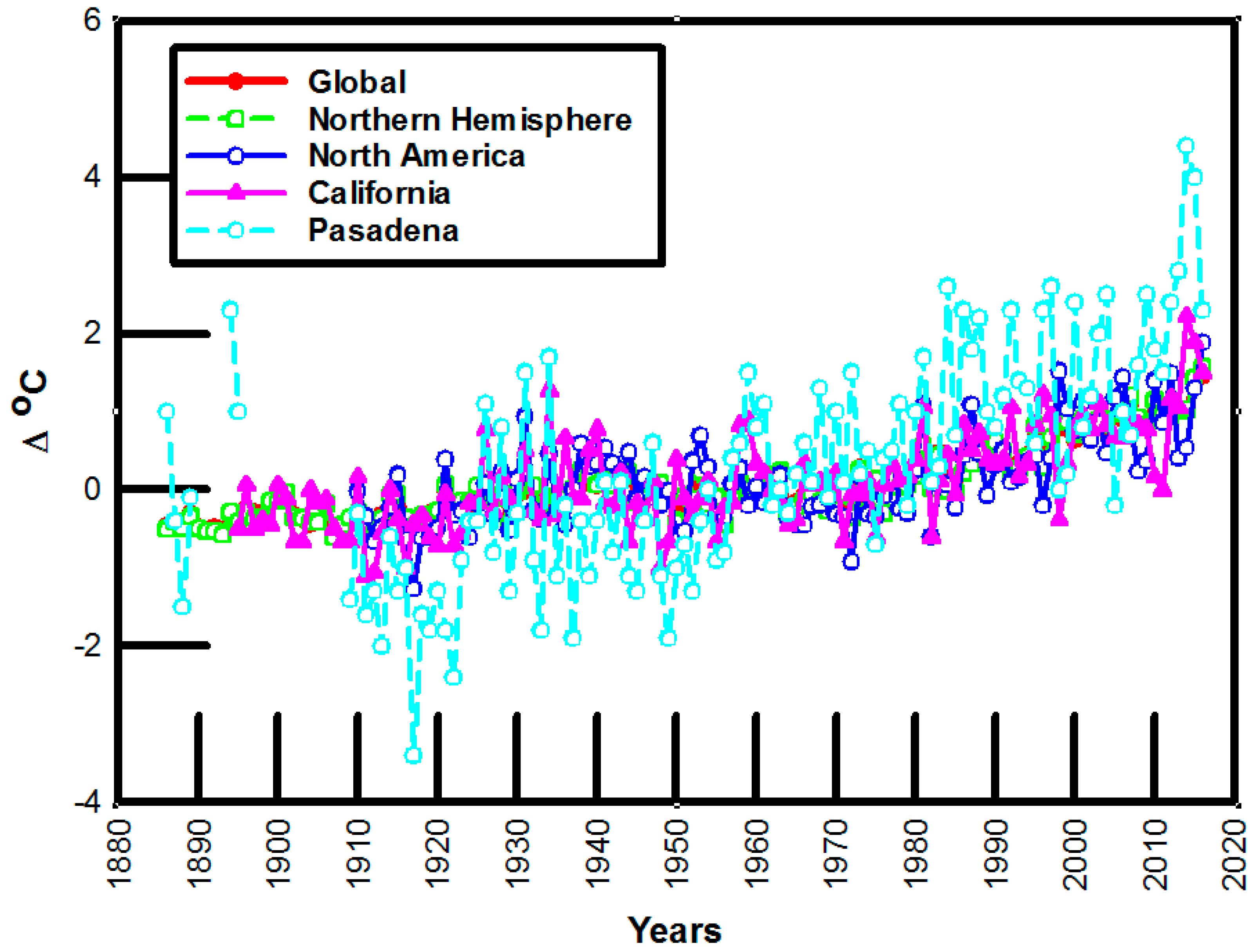
- Part 1: The average annual surface temperatures differences from the long term mean temperature were determined for each year between the Study Period. Then, the annual average temperature for each was compared to the average temperature of the Base Period. The difference between the annual average temperature of each year and the Base Period was calculated. This was done for the surface temperatures for the entire globe, the Northern Hemisphere, North America, California, and Pasadena. If the average annual temperature difference increased in parallel to changes seen in the broader data sets, there would be evidence for local climate change.
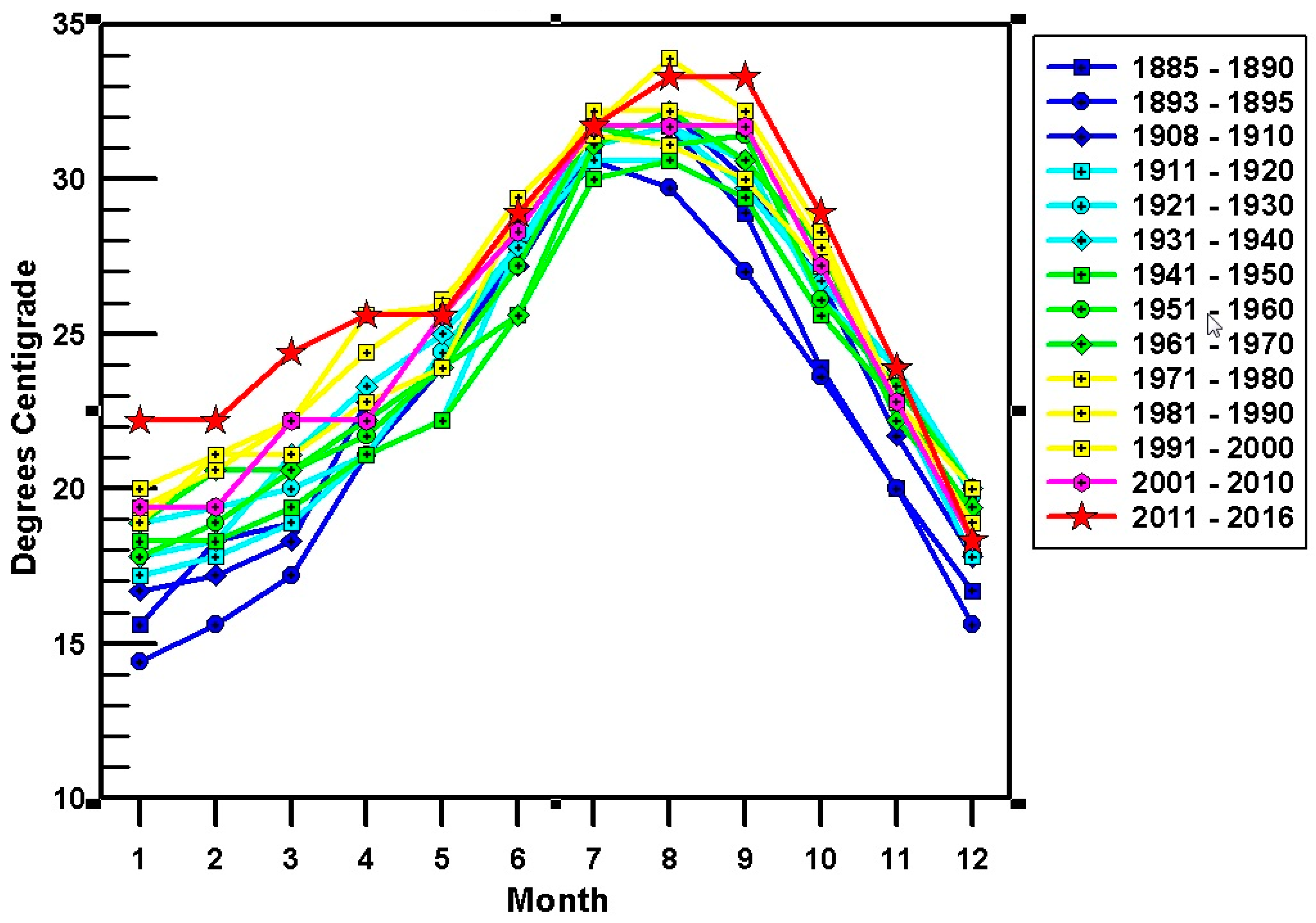
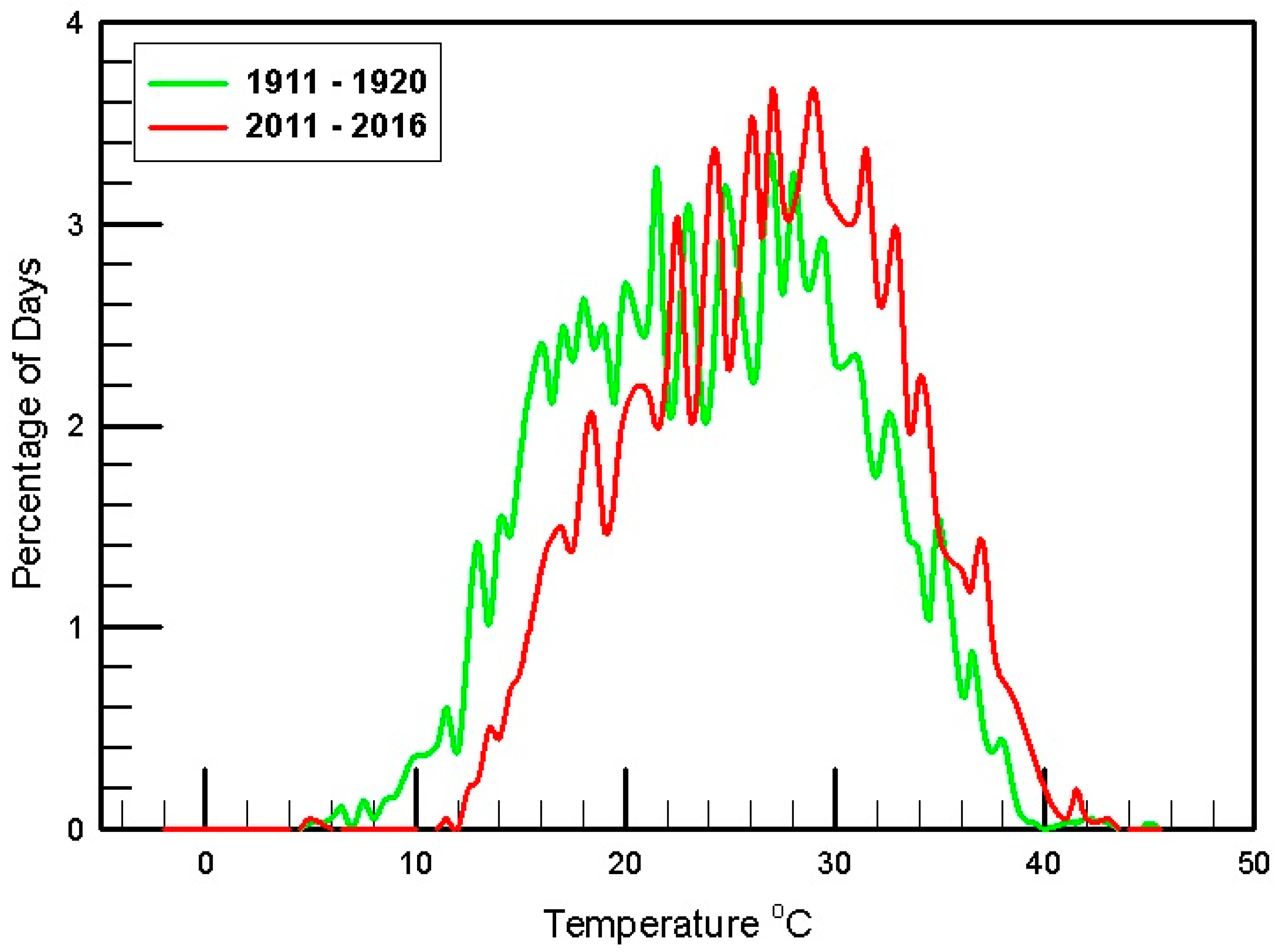
- Part 2: The daytime and nighttime temperatures for Pasadena were analyzed separately. If the daytime or nighttime temperatures increase or decrease significantly between 1885 and 2016, that would be an indication that climate change has been occurring. The record for 1885 was incomplete so it was not used in Part 1, but it would be useful for Part 2 for some months.
- Part 3: The second component involves measuring rainfall in the Pasadena area between 1883 and 2016 to determine if there has been a significant change in rainfall.
3.3. Statistical Procedures
- Normality. The normality of each data set was assessed using the Kolmogorov–Smirnov test. Air temperatures and rainfall in all study periods were non-normally distributed (p < 0.001); the results were strongly skewed and kurtotic. This means that rather than being distributed in a normal bell-shaped curve with data evenly balanced on both sides of the mean, more data was on one side than the other and the shape of the curve was wider than expected. Almost all of the data in this paper was non-normally distributed.
- Comparisons of Two Groups. When the rainfall and air temperature data were compared pairwise, the Mann–Whitney Rank Sum Test (MWRST) was used. This is the nonparametric equivalent to the Student’s t-test. The U values are calculated and the probability (p) that these represent significant differences was determined.
- Comparisons of More than Two Groups. The air temperature data was grouped based on decade and were compared to the most recent decade, the Kruskal–Wallis One-Way Analysis of Variance on Ranks (KW) was used. If a significant difference was determined to be present, i.e., if the Kruskal–Wallis Statistic (H) is above the critical value, then each group was compared against a control group using Dunn’s Test. Dunn’s Test produces a Studentized Range value, q, which is assessed in the same fashion as the Student’s t-test critical values with probabilities and critical values corresponding to levels of probability, α, of incorrectly rejecting the null hypothesis.
- Correlations. When temperature data from different locations was compared to determine if they tend to track each other, the Spearman Rank Order Correlation (SPOC) was used. The SPOC is the nonparametric equivalent to the Pearson Product Moment Correlation. The greater the correlation coefficient (R), the more the two sets of data track each other.
- Extreme Values. The rainfall data was also assessed for extremes. The number of driest and wettest months were calculated for each period using the Fisher Exact (FE) Test.
3.4. Data Acquisition and Assessment
- Air-PWP has extensive written records of atmospheric temperatures in Pasadena dating back to the 1880s, collected mostly by the employees of the City of Pasadena, but the records from 1882 to 1890 were collected by a private resident of Pasadena, Dr. Thomas Rigg. However, there are two significant gaps in the temperature records, one between 1890 and 1893 and the other between 1895 and 1908. The first gap is the time between when Dr. Rigg stopped collecting data and when the City started collecting data. The second gap was caused in part by the loss of paper records stored by the Department of Commerce in San Francisco following the earthquake and fire of 1906. The records were supplemented by and checked against records from the National Oceanic and Atmospheric Administration’s National Climatic Data Center (NOAA-NCDC). A database of the daily maximum temperature (all maximum temperatures occurred during the daylight hours are referred as “daytime temperatures”), minimum temperatures (all minimum temperatures occurred during the nighttime hours are referred as “nighttime temperatures”), and precipitation were created and checked for accuracy (paper records vs. electronic, missing data, and obvious outliers). A database of air temperatures was created with both the daytime (n = 41,201) and nighttime temperatures (n = 45,964) for Pasadena (most of the data was collected at City Hall, +34.15, −118.14 while other data were all collected within a kilometer of it). The temperature differences between the base period and each individual year was downloaded from the National Centers for Environmental information, Climate at a Glance: Global Time Series [8].
- Rainfall—The City of Pasadena began officially collecting rainfall data with its own staff in 1883 near the same location used for measuring temperature. Later, this site was coordinated with NOAA. Rainfall data was downloaded from the same webpage as the temperature data and the two databases were crosschecked.
4. Results
4.1. Part 1
4.2. Part 2
4.3. Rainfall
5. Discussion
6. Conclusions
Acknowledgments
Conflicts of Interest
References
- Kimbrough, D.E. Local Climate Change in Pasadena California and the Impact on Stream Flow. J. Am. Water W. Assoc. 2017, 109, E416–E425. [Google Scholar] [CrossRef]
- Los Angeles Basin Stormwater Conservation Study. Available online: https://www.usbr.gov/lc/socal/basinstudies/LABasin.html (accessed on 12 April 2018).
- Barsugli, J.J.; Guentchev, G.; Horton, R.M.; Wood, A.; Mearns, L.O.; Liang, X.-Z.; Winkler, J.A.; Dixon, K.; Hayhoe, K.; Rood, R.B.; et al. The Practitioner’s Dilemma: How to Assess the Credibility of Downscaled Climate Projections. Eos, Trans. Am. Geophys. Union 2013, 94, 424–425. [Google Scholar] [CrossRef]
- Sun, F.; Walton, D.; Hall, A. A hybrid dynamical–statistical downscaling technique, part II: End-of-century warming projections predict a new climate state in the Los Angeles region. J. Clim. 2015, 28, 4618–4636. [Google Scholar] [CrossRef]
- Hall, A. Projecting regional change. Science 2014, 346, 1461–1462. [Google Scholar] [CrossRef] [PubMed]
- Napton, D.E. Southern and Central California Chaparral and Oak Woodlands Ecoregion. In Status and Trends of Land Change in the Western United States—1973 to 2000; Benjamin, M.S., Tamara, S.W., William, A., Eds.; U.S. Geological Survey: Reston, VA, USA, 2012. [Google Scholar]
- De Muth, J.E. Basic Statistics and Pharmaceutical Statistical Applications, 3rd ed.; CRC Press: Boca Raton, FL, USA, 2014; pp. 242–244. ISBN 9781466596733. [Google Scholar]
- National Oceanic and Atmospheric Administration. Climate at a Glance: Global Time Series. Available online: https://www.ncdc.noaa.gov/cag/ (accessed on 10 April 2018).
- Edinger, J.G. Modication of Marine Layer over Southern California. J. Appl. Meteorol. 1963, 2, 706–712. [Google Scholar] [CrossRef]
- Terjung, W.H.; O’Rourke, P.A. Influences of Physical Structures on Urban Energy Budgets. Bound. Layer Meteorol. 1980, 19, 421–439. [Google Scholar] [CrossRef]
- Hatzianastassiou, N.; Fotiadi, A.; Matsoukas, C.; Pavlakis, K.G.; Drakakis, E.; Hatzidimitriou, D.; Vardavas, I. Long-term global distribution of Earth’s shortwave radiation, budget at the top of atmosphere. Atmos. Chem. Phys. 2004, 4, 1217–1235. [Google Scholar] [CrossRef]


| Location | Period | n | Mean | 50th | 25th | 75th | MWRST | ||
|---|---|---|---|---|---|---|---|---|---|
| Percentile | U | T | p | ||||||
| Global | 1886–2016 | 131 | 0.08 | −0.03 | −0.26 | 0.27 | |||
| 1886–1949 | 64 | −0.21 | −0.21 | −0.38 | −0.03 | ||||
| 1950–2016 | 67 | 0.35 | 0.23 | −0.05 | 0.80 | 567 | 2647 | <0.001 | |
| Norther Hemisphere | 1886–2016 | 131 | 0.08 | −0.03 | −0.29 | 0.26 | |||
| 1886–1949 | 64 | −0.20 | −0.19 | −0.39 | 0.01 | ||||
| 1950–2016 | 67 | 0.35 | 0.23 | −0.05 | 0.84 | 428 | 2808 | <0.001 | |
| North America | 1910–2016 | 107 | 0.14 | 0.080 | −0.31 | 0.46 | |||
| 1886–1949 | 40 | −0.20 | −0.19 | −0.39 | 0.01 | ||||
| 1950–2016 | 67 | 0.28 | 0.24 | −0.21 | 0.64 | 871 | 1691 | 0.003 | |
| California | 1895–2016 | 122 | 0.10 | 0.03 | −0.39 | 0.50 | |||
| 1886–1949 | 55 | −0.24 | −0.28 | −0.56 | 0.00 | ||||
| 1950–2016 | 67 | 0.35 | 0.33 | 0.00 | 0.83 | 704 | 2244 | <0.001 | |
| Pasadena | 1886–2016 * | 114 | 0.29 | 0.15 | −0.80 | 1.23 | |||
| 1886–1949 * | 47 | −0.68 | −0.90 | −1.40 | 0.20 | ||||
| 1950–2016 | 67 | 0.98 | 0.80 | 0.10 | 1.80 | 457 | 1585 | <0.001 | |
| Norther Hemisphere | North America | California | Pasadena | ||||||
| Global | R | 0.99 | 0.81 | 0.69 | 0.64 | ||||
| p | <0.0001 | <0.0001 | <0.0001 | <0.0001 | |||||
| Norther Hemisphere | R | 0.84 | 0.67 | 0.59 | |||||
| p | <0.0001 | <0.0001 | <0.0001 | ||||||
| North America | R | 0.60 | 0.54 | ||||||
| p | <0.0001 | <0.0001 | |||||||
| California | R | 0.79 | |||||||
| p | <0.0001 | ||||||||
| Months | Period | n | Mean | 50th | 25th | 75th | % Change in Median | MWRSTU Value | Probability |
|---|---|---|---|---|---|---|---|---|---|
| All | Study | 41,890 | 25.0 | 25.0 | 20.0 | 30.0 | |||
| Control | 17,590 | 24.2 | 24.4 | 19.4 | 29.4 | ||||
| Test | 24,299 | 25.5 | 25.6 | 20.6 | 30.6 | 5 | 190,921,246 | <0.001 | |
| January | Study | 3580 | 19.1 | 18.9 | 15.6 | 22.8 | |||
| Control | 1505 | 18.1 | 17.8 | 14.4 | 22.2 | ||||
| Test | 2075 | 25.5 | 19.4 | 16.1 | 23.3 | 9 | 1,258,874 | <0.001 | |
| February | Study | 3213 | 20.0 | 19.4 | 16.1 | 23.3 | |||
| Control | 1320 | 18.6 | 18.3 | 15.0 | 21.7 | ||||
| Test | 1893 | 20.9 | 20.6 | 17.2 | 24.4 | 13 | 919,116 | <0.001 | |
| March | Study | 3225 | 21.2 | 20.6 | 17.8 | 24.4 | |||
| Control | 1458 | 20.1 | 19.4 | 16.7 | 23.3 | ||||
| Test | 2067 | 21.9 | 21.7 | 18.3 | 25.0 | 5 | 2,245,290 | <0.001 | |
| April | Study | 3377 | 23.0 | 22.8 | 19.4 | 26.7 | |||
| Control | 1380 | 22.0 | 21.7 | 18.3 | 25.6 | ||||
| Test | 1997 | 23.8 | 23.3 | 20.0 | 27.2 | 7 | 1,107,918 | <0.001 | |
| May | Study | 3514 | 24.7 | 24.4 | 21.7 | 27.8 | |||
| Control | 1452 | 23.9 | 23.3 | 20.6 | 26.7 | ||||
| Test | 2052 | 25.3 | 25.0 | 22.2 | 28.3 | 7 | 1,239,675 | <0.001 | |
| June | Study | 3378 | 27.7 | 27.8 | 25.0 | 30.6 | |||
| Control | 1410 | 27.2 | 27.2 | 24.4 | 30.0 | ||||
| Test | 1968 | 28.2 | 28.3 | 25.0 | 31.1 | 4 | 1,209,085 | <0.001 | |
| July | Study | 3558 | 31.4 | 31.1 | 29.4 | 33.3 | |||
| Control | 1492 | 31.0 | 31.1 | 28.9 | 32.8 | ||||
| Test | 2066 | 31.6 | 31.7 | 29.4 | 33.3 | 2 | 1,348,717 | <0.001 | |
| August | Study | 3612 | 31.8 | 31.7 | 29.4 | 33.9 | |||
| Control | 1549 | 31.3 | 31.1 | 28.9 | 33.9 | ||||
| Test | 2063 | 32.2 | 32.2 | 30.0 | 34.4 | 4 | 1,358,929 | <0.001 | |
| September | Study | 3500 | 30.7 | 30.6 | 27.2 | 33.9 | |||
| Control | 1500 | 29.7 | 29.4 | 26.7 | 32.8 | ||||
| Test | 2000 | 31.4 | 31.7 | 27.8 | 34.4 | 8 | 1,189,293 | <0.001 | |
| October | Study | 3587 | 27.0 | 26.7 | 23.3 | 30.6 | |||
| Control | 1519 | 25.9 | 25.6 | 22.2 | 29.4 | ||||
| Test | 2068 | 27.8 | 27.2 | 23.9 | 31.1 | 6 | 1,255,054 | <0.001 | |
| November | Study | 3387 | 23.1 | 22.8 | 19.4 | 26.7 | |||
| Control | 1525 | 23.0 | 22.8 | 19.4 | 26.7 | ||||
| Test | 1982 | 23.2 | 22.8 | 20.0 | 26.7 | 0 | 1,483,766 | 0.35 | |
| December | Study | 3563 | 19.5 | 18.9 | 16.1 | 22.8 | |||
| Control | 1519 | 19.1 | 18.9 | 15.6 | 22.8 | ||||
| Test | 2044 | 19.8 | 19.4 | 16.7 | 22.8 | 2 | 1,409,343 | <0.001 |
| Months | Period | n | Mean | 50th | 25th | 75th | % Change in Median | MWRSTU Value | Probability |
|---|---|---|---|---|---|---|---|---|---|
| All | Study | 41,856 | 10.7 | 10.6 | 10.6 | 7.20 | |||
| Control | 17,588 | 9.4 | 9.4 | 6.1 | 12.8 | ||||
| Test | 24,268 | 11.6 | 11.7 | 8.3 | 15.0 | 24 | 58,789,490 | <0.001 | |
| January | Study | 3579 | 6.0 | 6.1 | 3.9 | 8.3 | |||
| Control | 1505 | 4.6 | 4.4 | 2.2 | 6.7 | ||||
| Test | 2074 | 7.0 | 7.2 | 5.0 | 9.4 | 64 | 917,958 | <0.001 | |
| February | Study | 3213 | 6.8 | 6.7 | 4.4 | 8.9 | |||
| Control | 1320 | 5.5 | 5.6 | 3.3 | 7.8 | ||||
| Test | 1893 | 7.8 | 7.8 | 5.6 | 10.0 | 39 | 748,569 | <0.001 | |
| March | Study | 3525 | 7.9 | 7.8 | 5.6 | 10.0 | |||
| Control | 1458 | 6.8 | 6.7 | 4.4 | 8.9 | ||||
| Test | 2067 | 8.6 | 8.9 | 6.7 | 10.6 | 33 | 953,700 | <0.001 | |
| April | Study | 3372 | 9.5 | 9.4 | 7.8 | 11.7 | |||
| Control | 1380 | 8.5 | 8.9 | 6.7 | 10.6 | ||||
| Test | 1998 | 10.1 | 10.0 | 8.3 | 12.2 | 12 | 953,700 | <0.001 | |
| May | Study | 3513 | 11.4 | 11.7 | 9.4 | 13.3 | |||
| Control | 1452 | 10.3 | 10.6 | 8.3 | 12.2 | ||||
| Test | 2061 | 12.2 | 12.2 | 10.6 | 13.9 | 15 | 931,875 | <0.001 | |
| June | Study | 3377 | 13.3 | 13.3 | 11.7 | 15.0 | |||
| Control | 1410 | 12.0 | 12.2 | 10.6 | 13.9 | ||||
| Test | 1977 | 14.3 | 14.4 | 12.8 | 15.6 | 18 | 700,701 | <0.001 | |
| July | Study | 3553 | 15.6 | 15.6 | 13.9 | 17.2 | |||
| Control | 1492 | 14.3 | 14.4 | 12.8 | 16.1 | ||||
| Test | 2064 | 16.6 | 16.7 | 15.0 | 18.3 | 16 | 779,121 | <0.001 | |
| August | Study | 3598 | 15.8 | 15.6 | 13.9 | 17.8 | |||
| Control | 1549 | 14.4 | 14.4 | 12.2 | 16.1 | ||||
| Test | 2047 | 16.9 | 16.7 | 15.0 | 18.3 | 16 | 780,254 | <0.001 | |
| September | Study | 3499 | 15.0 | 14.4 | 12.5 | 16.7 | |||
| Control | 1500 | 13.1 | 12.8 | 11.1 | 15.0 | ||||
| Test | 1999 | 16.1 | 16.1 | 13.9 | 17.8 | 26 | 729,880 | <0.001 | |
| October | Study | 3584 | 12.0 | 12.2 | 10.0 | 14.4 | |||
| Control | 1519 | 10.4 | 12.2 | 10.0 | 14.4 | ||||
| Test | 2065 | 13.2 | 13.3 | 11.1 | 15.0 | 9 | 808,120 | <0.001 | |
| November | Study | 3388 | 8.54 | 8.3 | 6.1 | 11.1 | |||
| Control | 1525 | 7.48 | 7.2 | 5.0 | 9.4 | ||||
| Test | 1983 | 9.45 | 9.4 | 7.2 | 11.7 | 31 | 988,824 | <0.001 | |
| December | Study | 3561 | 6.4 | 6.1 | 4.4 | 8.3 | |||
| Control | 1519 | 5.5 | 5.6 | 3.3 | 7.8 | ||||
| Test | 2042 | 7.0 | 7.2 | 5.0 | 8.9 | 29 | 1,131,512 | <0.001 |
| Months | Period | Years | n | Mean | 50th | 25th | 75th | Driest Months | Wettest Months | Median MWRST | Driest FE | Wettest FE | |
|---|---|---|---|---|---|---|---|---|---|---|---|---|---|
| U | P | P | P | ||||||||||
| All | Study | 1883–2016 | 134 | 508 | 456 | 334 | 648 | 395 | 100 | ||||
| Control | 1883–1949 | 67 | 523 | 462 | 361 | 657 | 194 | 53 | |||||
| Test | 1950–2016 | 67 | 491 | 411 | 289 | 628 | 201 | 47 | 1957 | 0.202 | |||
| October | Study | 1883–2016 | 134 | 19.4 | 11.4 | 1.0 | 24.6 | 23 | 10 | ||||
| Control | 1883–1949 | 67 | 22.0 | 12.4 | 2.3 | 25.4 | 8 | 8 | |||||
| Test | 1950–2016 | 67 | 16.8 | 8.9 | 0.3 | 23.4 | 15 | 2 | 1944 | 0.181 | 0.20 | 0.20 | |
| November | Study | 1883–2016 | 134 | 43.1 | 25.5 | 4.0 | 61.6 | 14 | 10 | ||||
| Control | 1883–1949 | 67 | 38.8 | 18.5 | 3.8 | 53.1 | 8 | 6 | |||||
| Test | 1950–2016 | 67 | 47.3 | 33.8 | 4.3 | 64.8 | 6 | 4 | 1945 | 0.182 | 0.6 | 0.75 | |
| December | Study | 1883–2016 | 134 | 80.1 | 51.3 | 19.1 | 122 | 10 | 10 | ||||
| Control | 1883–1949 | 67 | 91.2 | 68.6 | 24.1 | 126 | 5 | 8 | |||||
| Test | 1950–2016 | 67 | 69.1 | 40.4 | 16.8 | 112 | 5 | 2 | 1957 | 0.201 | 1.0 | 0.18 | |
| January | Study | 1883–2016 | 134 | 105 | 73.7 | 25.0 | 156 | 10 | 10 | ||||
| Control | 1883–1949 | 67 | 101 | 75.2 | 23.6 | 159 | 5 | 5 | |||||
| Test | 1950–2016 | 67 | 110 | 72.1 | 25.7 | 152 | 5 | 5 | 2174 | 0.757 | 1.0 | 1.0 | |
| February | Study | 1883–2016 | 134 | 110 | 68.7 | 27.8 | 162 | 10 | 10 | ||||
| Control | 1883–1949 | 67 | 110 | 76.5 | 27.9 | 162 | 6 | 4 | |||||
| Test | 1950–2016 | 67 | 111 | 62.2 | 25.9 | 163 | 4 | 6 | 2162 | 0.717 | 0.75 | 0.75 | |
| March | Study | 1883–2016 | 134 | 88.1 | 60.7 | 25.3 | 122 | 10 | 10 | ||||
| Control | 1883–1949 | 67 | 96.0 | 73.9 | 24.4 | 133 | 4 | 8 | |||||
| Test | 1950–2016 | 67 | 80.6 | 55.6 | 25.9 | 112 | 6 | 2 | 2028 | 0.338 | 0.75 | 0.20 | |
| April | Study | 1883–2016 | 134 | 36.1 | 18.0 | 8.3 | 52.5 | 13 | 10 | ||||
| Control | 1883–1949 | 67 | 36.4 | 18.8 | 9.7 | 52.3 | 1 | 4 | |||||
| Test | 1950–2016 | 67 | 35.8 | 17.5 | 3.8 | 52.8 | 12 * | 6 | 2095 | 0.509 | 0.003 | 0.75 | |
© 2018 by the author. Licensee MDPI, Basel, Switzerland. This article is an open access article distributed under the terms and conditions of the Creative Commons Attribution (CC BY) license (http://creativecommons.org/licenses/by/4.0/).
Share and Cite
Kimbrough, D.E. Changes in Temperature and Rainfall as a Result of Local Climate Change in Pasadena, California. Hydrology 2018, 5, 25. https://doi.org/10.3390/hydrology5020025
Kimbrough DE. Changes in Temperature and Rainfall as a Result of Local Climate Change in Pasadena, California. Hydrology. 2018; 5(2):25. https://doi.org/10.3390/hydrology5020025
Chicago/Turabian StyleKimbrough, David Eugene. 2018. "Changes in Temperature and Rainfall as a Result of Local Climate Change in Pasadena, California" Hydrology 5, no. 2: 25. https://doi.org/10.3390/hydrology5020025
APA StyleKimbrough, D. E. (2018). Changes in Temperature and Rainfall as a Result of Local Climate Change in Pasadena, California. Hydrology, 5(2), 25. https://doi.org/10.3390/hydrology5020025


