Assessment of Future Water Resources Availability under Climate Change Scenarios in the Mékrou Basin, Benin

Abstract
1. Introduction
2. Data and Methods
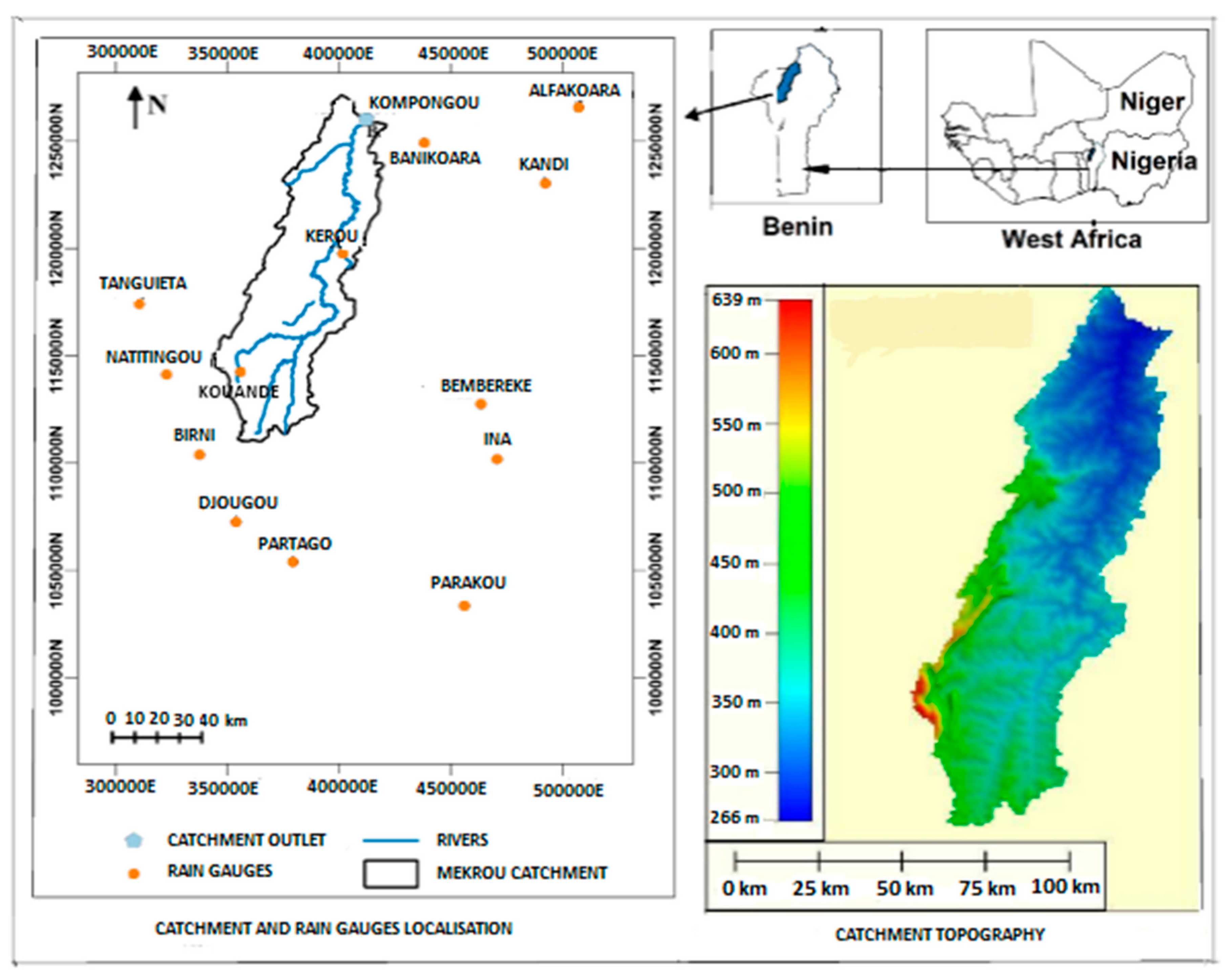
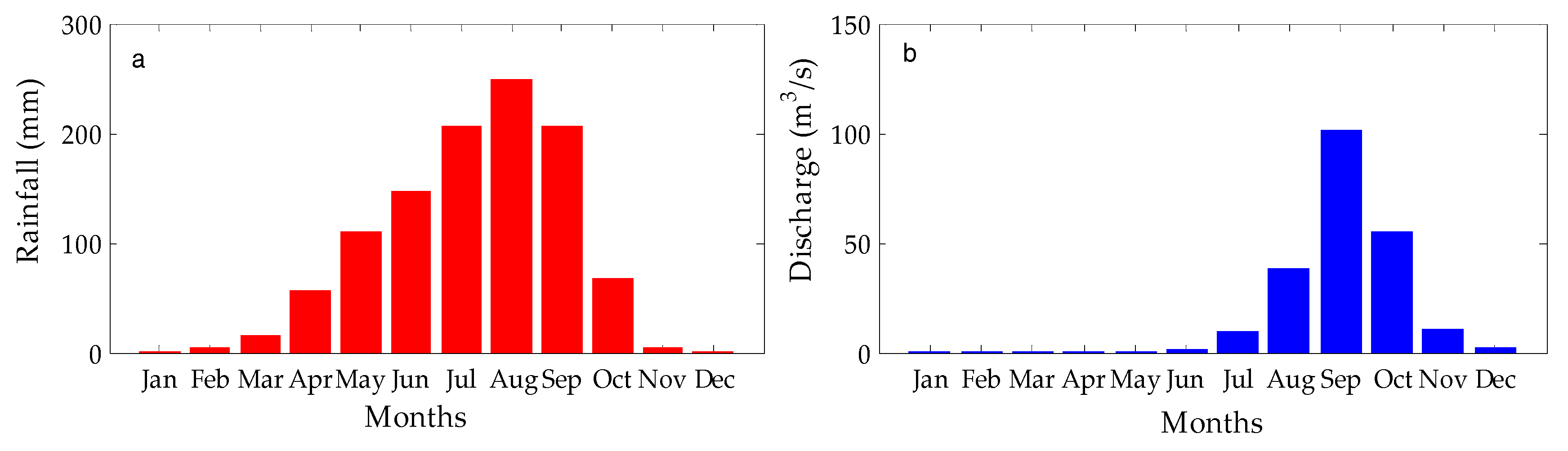
2.1. Study Area
2.2. Data
2.3. Methodology
2.3.1. Bias Corrected Method
2.3.2. Rainfall Interpolation Method
2.3.3. Potential Evapotranspiration (PET) Estimation Method
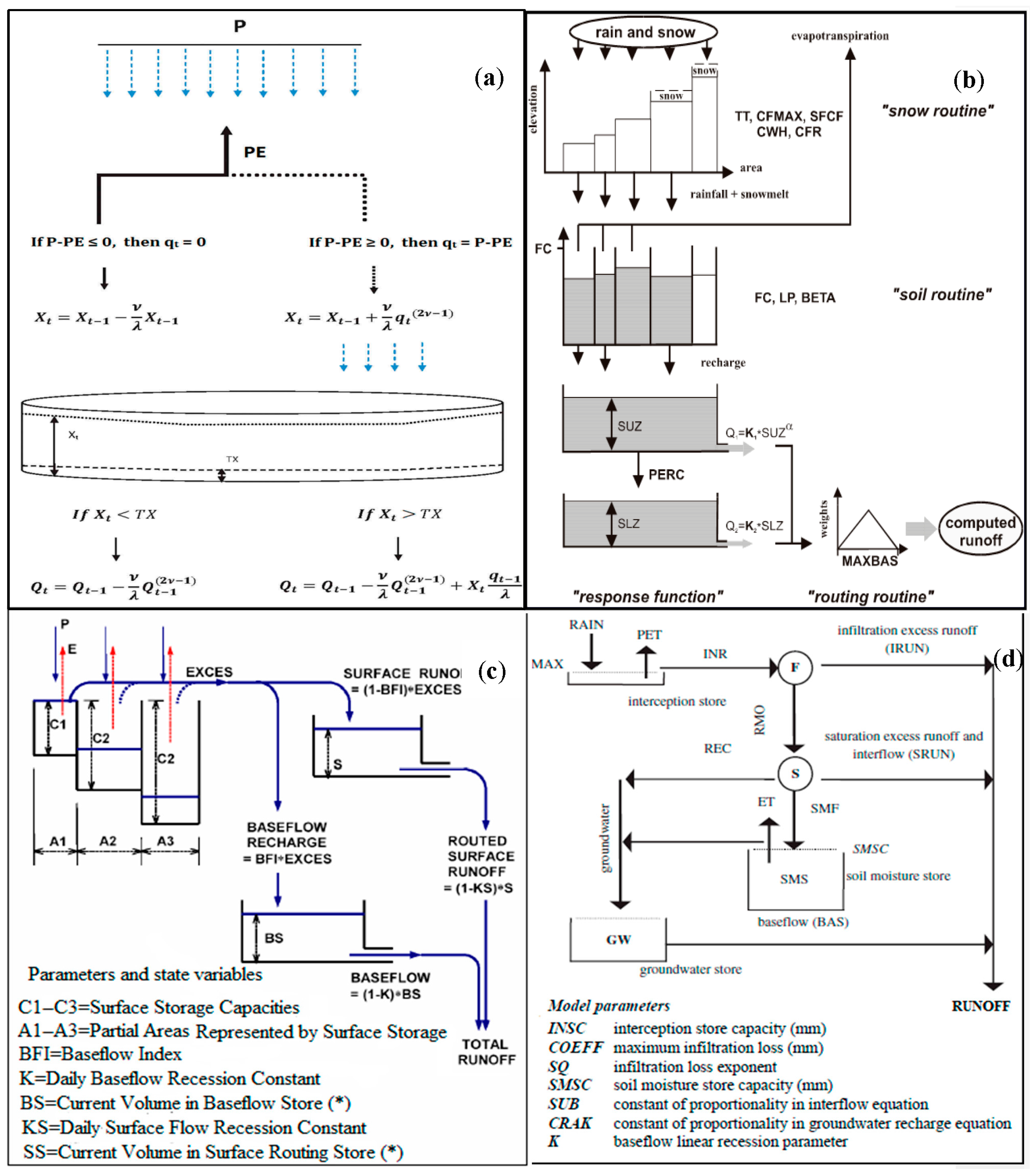
2.3.4. Hydrological Models
- (a)
- From day t − 1 to day t, the state X of the soil changes and Xt depends on Xt−1 .
- (b)
- The state of the soil is modified by the occurrence of precipitation: Xt is a function of Xt−1 and qt.
- (c)
- The state of the soil Xt does not contribute to the discharge of day t as long as it is smaller than a threshold value TX.
2.3.5. Calibration Procedure
2.3.6. Change Rates
2.3.7. Student’s t-Test
3. Results
3.1. Change in Rainfall
3.1.1. Annual Change
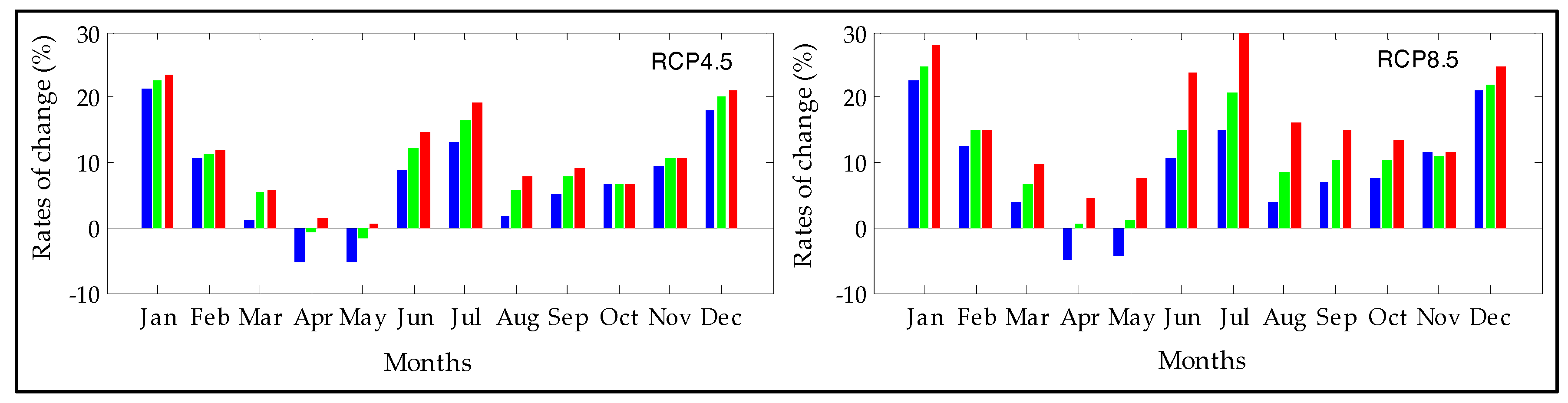
3.1.2. Monthly Change
3.2. Potential Evapotranspiration Change
3.2.1. Annual Change
3.2.2. Monthly Change
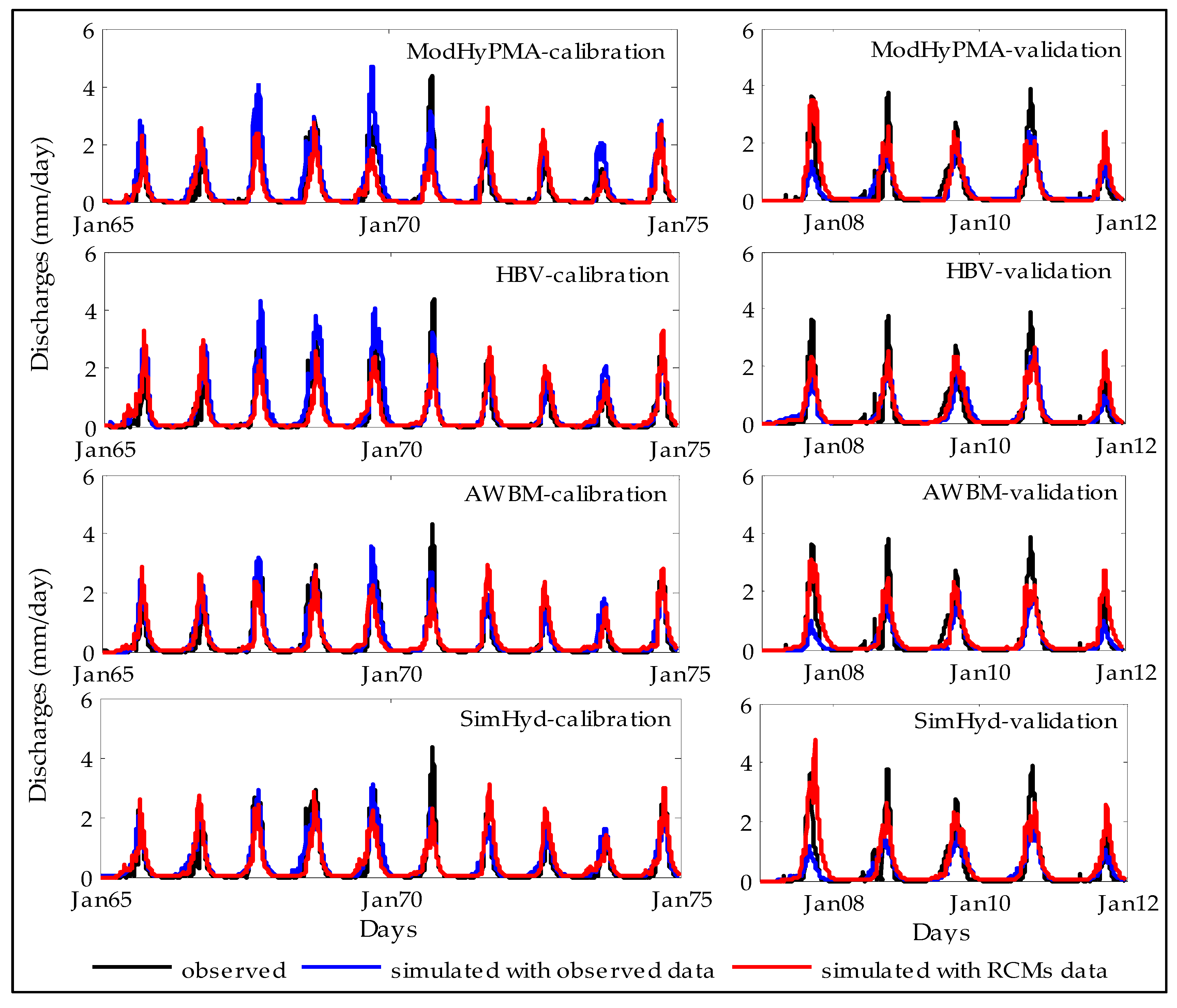
3.3. Discharges Simulation
Performances of Hydrological Models
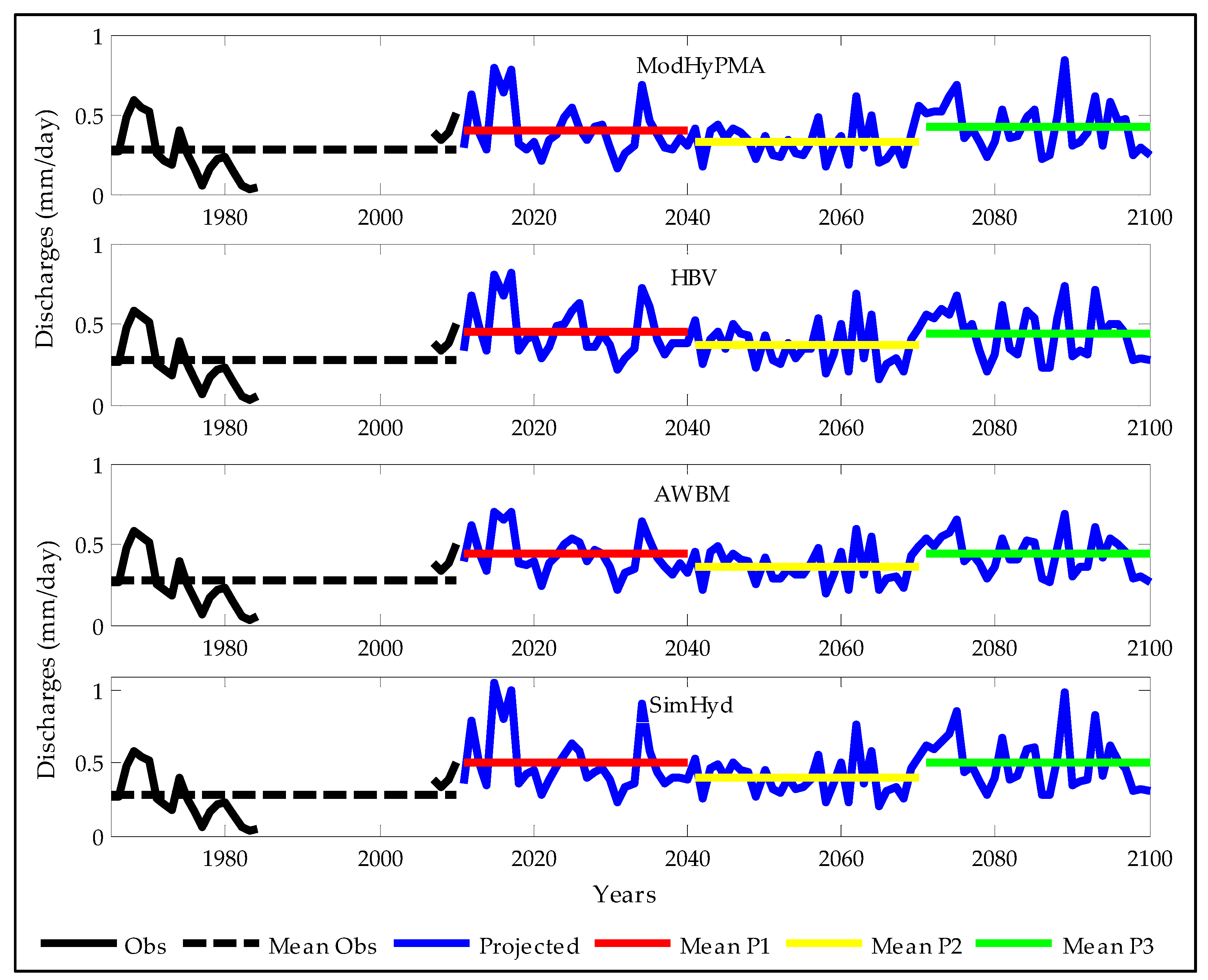
3.4. Change in Runoff
3.4.1. Annual Change
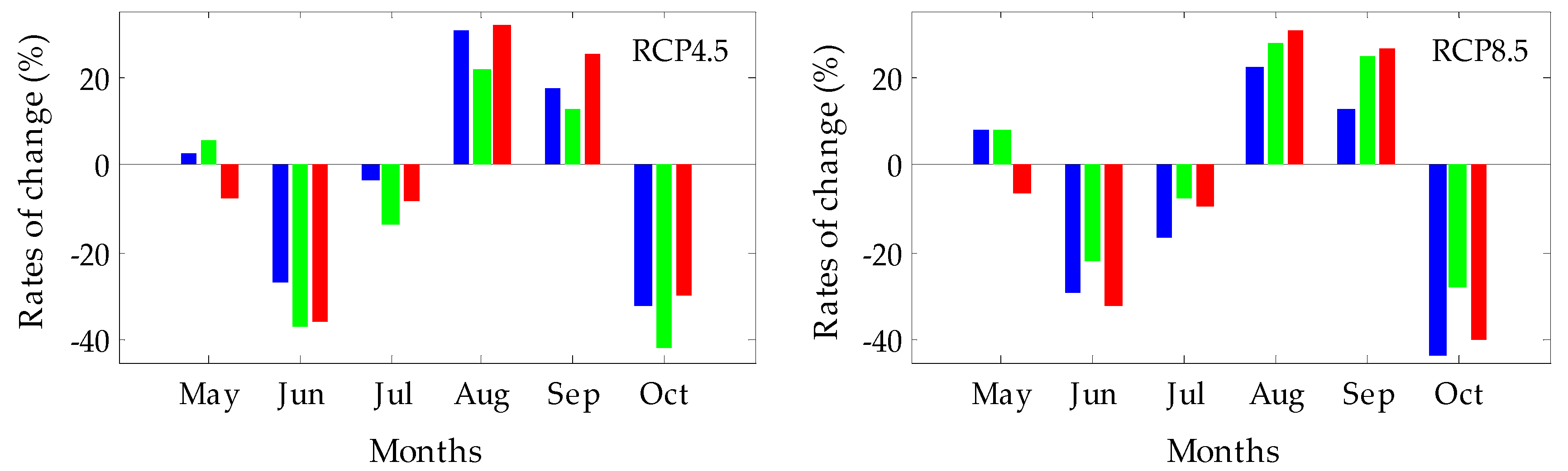
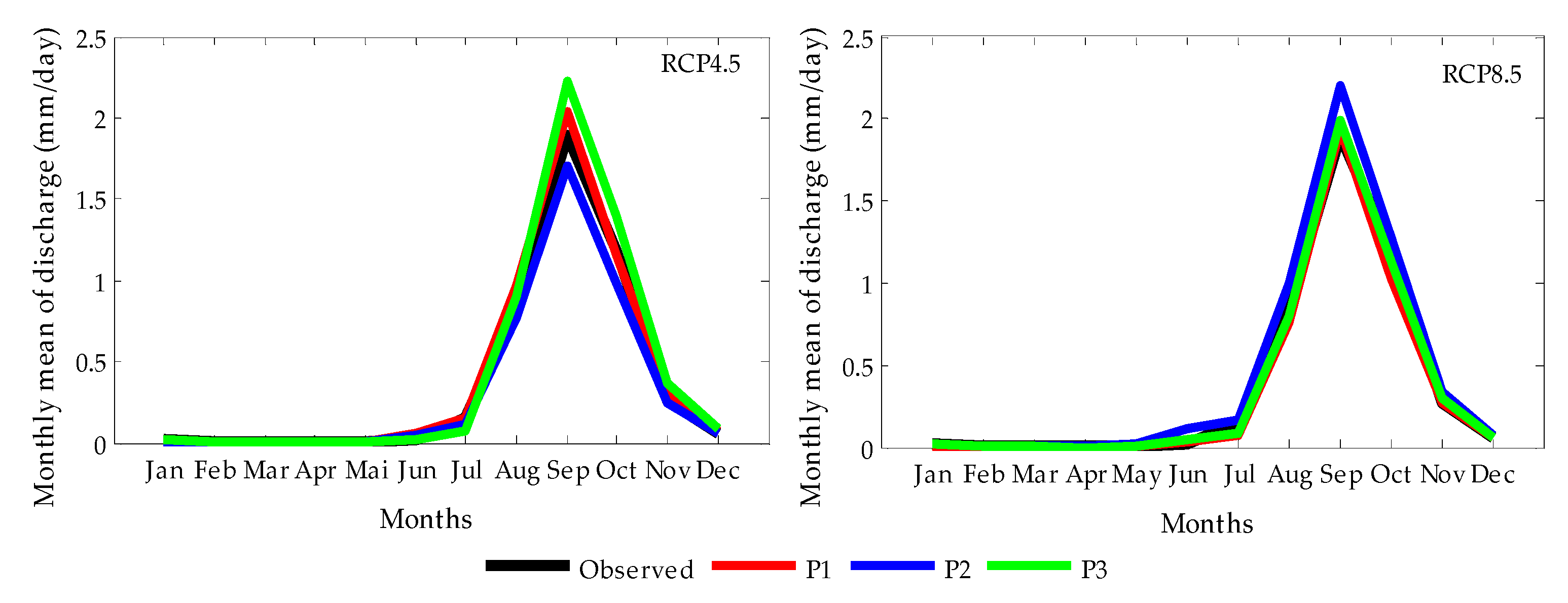
3.4.2. Monthly Change
4. Discussion
5. Conclusions
Acknowledgments
Author Contributions
Conflicts of Interest
References
- Intergovernmental Panel on Climate Change (IPCC). Summary for Policymakers. In Climate Change 2014: Impacts, Adaptation, and Vulnerability; Contribution of Working Group II to the Fifth Assessment Report of the Intergovernmental Panel on Climate Change; Cambridge University Press: Cambridge, UK; New York, NY, USA, 2014. [Google Scholar]
- Barrios, S.; Ouattara, B.; Strobl, E. The impact of climatic change on agricultural production: Is it different for Africa? Food Policy 2008, 33, 287–298. [Google Scholar] [CrossRef]
- Giorgi, F.; Coppola, E.; Raffaele, F. A consistent picture of the hydroclimatic response to global warming from multiple indices: Models and observations. J. Geophys. Res. Atmos. 2014, 119. [Google Scholar] [CrossRef]
- Zwiers, F.W.; Alexander, L.V.; Hegerl, G.C.; Knutson, T.R.; Kossin, J.; Naveau, P.; Nicholls, N.; Schär, C.; Seneviratne, S.I.; Zhang, X. Challenges in estimating and understanding recent changes in the frequency and intensity of extreme climate and weather events. In Climate Science for Serving Society: Research, Modeling and Prediction Priorities; Springer: Berlin, Germany, 2013. [Google Scholar]
- Intergovernmental Panel on Climate Change (IPCC). Climate Change 2007—Synthesis Report; Cambridge University Press: Cambridge, UK, 2007. [Google Scholar]
- Sylla, M.B.; Nikiema, P.M.; Gibba, P.; Kebe, I.; Klutse, N.A.B. Climate change over West Africa: Recent trends and future projections. In Adaptation to Climate Change and Variability in Rural West Africa; Springer: Basel, Switzerland, 2016. [Google Scholar]
- Sylla, M.B.; Elguindi, N.; Giorgi, F.; Wisser, D. Projected robust shift of climate zones over West Africa in response to anthropogenic climate change for the late 21st century. Clim. Chang. 2016, 134, 241–253. [Google Scholar] [CrossRef]
- Tall, M.; Sylla, M.B.; Diallo, I.; Pal, J.S.; Faye, A.; Mbaye, M.L.; Gaye, A.T. Projected impact of climate change in the hydroclimatology of Senegal with a focus over the Lake of Guiers for the twenty-first century. Theor. Appl. Climatol. 2017, 129, 655–665. [Google Scholar] [CrossRef]
- Obada, E.; Alamou, E.A.; Zandagba, E.J.; Chabi, A.; Afouda, A. Change in future rainfall characteristics in the Mekrou Catchment (Benin), from an ensemble of 3 RCMs (MPI-REMO, DMI-HIRHAM5 and SMHI-RCA4). Hydrology 2017, 4, 14. [Google Scholar] [CrossRef]
- Ibrahim, B.; Karambiri, H.; Polcher, J.; Yacouba, H.; Ribstein, P. Changes in rainfall regime over Burkina Faso under the climate change conditions simulated by 5 regional climate models. Clim. Dyn. 2014, 42, 1363–1381. [Google Scholar] [CrossRef]
- Cook, K.H.; Vizy, E.K. Impact of climate change on mid-twenty-first century growing seasons in Africa. Clim. Dyn. 2012, 39, 2937–2955. [Google Scholar] [CrossRef]
- Elguindi, N.; Grundstein, A.; Bernardes, S.; Turuncoglu, U.; Feddema, J. Assessment of CMIP5 global model simulations and climate change projections for the 21st Century using a modified Thornthwaite climate classification. Clim. Chang. 2014, 122, 523–538. [Google Scholar] [CrossRef]
- Akinsanola, A.A.; Ogunjobi, K.O.; Gbode, I.E.; Ajayi, V.O. Assessing the capabilities of three regional climate models over CORDEX Africa in simulating West African summer monsoon precipitation. Adv. Meteorol. 2015, 2015, 935431. [Google Scholar] [CrossRef]
- Yira, Y.; Diekkrüger, B.; Steup, G.; Bossa, A.Y. Impact of climate change on hydrological conditions in a tropical West African catchment using an ensemble of climate simulations. Hydrol. Earth Syst. Sci. 2017, 21, 2143–2161. [Google Scholar] [CrossRef]
- Sarr, A.B.; Camara, M.; Diba, I. Spatial distribution of cordex regional climate models biases over West Africa. Int. J. Geosci. 2015, 6, 1018–1031. [Google Scholar] [CrossRef]
- GLEauBe. Etude Portant État Des Lieux et Gestion de L’information sur les Ressources en eau Dans le Bassin de la Mékrou; Rapport Technique: Cotonou, Benin, 2012; p. 104. [Google Scholar]
- Benoit, M. Statut et Usages du sol en Périphérie du Parc National du “w ” du Niger. Tome 1 Contribution à L’étude du Milieu Naturel et des Ressources Végétales du Canton de Tamou et du Parc du ”W ”; ORSTOM: Bondy, France, 1998. [Google Scholar]
- Christensen, O.B.; Drews, M.; Christensen, J.H. The HIRHAM Regional Climate Model Version 5. Available online: http://orbit.dtu.dk/fedora/objects/orbit:118724/datastreams/file_8c69af6e-acfb-4d1aaa53-73188c001d36/content (accessed on 15 February 2017).
- Jacob, D.; Bärring, L.; Christensen, O.B.; Christensen, J.H.; Hagemann, S.; Hirschi, M.; Kjellström, E.; Lenderink, G.; Rockel, B.; Schär, C.; et al. An inter-comparison of regional climate models for Europe: Design of the experiments and model performance. Clim. Chang. 2007, 81, 31–52. [Google Scholar] [CrossRef]
- Samuelsson, P.; Jones, C.G.; Willén, U.; Ullerstig, A.; Gollvik, S.; Hansson, U.; Kjellström, E.; Nikulin, G.; Wyser, K. The Rossby Centre regional climate model RCA3: Model description and performance. Tellus A 2011, 63, 4–23. [Google Scholar] [CrossRef]
- Obada, E.; Alamou, A.E.; Zandagba, E.J.; Biao, I.E.; Chabi, A.; Afouda, A. Comparative study of seven bias correction methods applied to three Regional Climate Models in Mekrou Catchment (Benin, West Africa). IJCET 2016, 6, 1831–1840. [Google Scholar]
- Déqué, M. Frequency of precipitation and temperature extremes over France in an anthropogenic scenario: Model results and statistical correction according to observed values. Glob. Planet. Chang. 2007, 57, 16–26. [Google Scholar] [CrossRef]
- Arnaud, M.; Emery, X. Estimation and Spatial Interpolation: Deterministic Methods and Geostatistics Methods; Hermès: Paris, France, 2000; p. 221. [Google Scholar]
- Cressie, N. Statistics for Spatial Data; Wiley: New York, NY, USA, 1992; pp. 613–617. [Google Scholar]
- Matheron, G. Regionalized variables theory and its applications. In Note Book of Mathematical Morphology Centre; Fasc. 5 EMP: Paris, France, 1971; p. 212. [Google Scholar]
- Allen, R.; Periera, L.; Raes, D.; Smith, M. FAO Irrigation and Drainage: Crop Evapotranspiration (Guidelines for Computing Crop Water Requirements); Paper No. 56; FAO: Rome, Italy, 1996. [Google Scholar]
- Afouda, A.; Alamou, A.E. Modèle hydrologique basé sur le Principe de Moindre Action (ModHyPMA). Ann. Sci. Agron. 2010, 13, 23–45. [Google Scholar] [CrossRef]
- Bergström, S.; Forsman, A. Development of a conceptual deterministic rainfall runoff model. Nord. Hydrol. 1973, 14, 147–170. [Google Scholar]
- Boughton, W.C. An Australian water balance model for semiarid watersheds. J. Soil Water Conserv. 1995, 50, 454–457. [Google Scholar]
- Boughton, W. The Australian water balance model. Environ. Model. Softw. 2004, 19, 943–956. [Google Scholar] [CrossRef]
- Chiew, F.H.S.; Siriwardena, L. Estimation of SIMHYD parameter values for application in ungauged catchments. In Proceedings of the MOD-SIM 2005 International Congress on Modelling and Simulation. Modelling and Simulation Society of Australia and New Zealand, Melbourne, Australia, December 2005; pp. 2883–2889. [Google Scholar]
- Alamou, A.E. Application du Principe de Moindre Action à la Modélisation Pluie-Débit. Ph.D. Thesis, Université d’Abomey Calavi, Abomey Calavi, Benin, 2011; p. 231. [Google Scholar]
- Gaba, C.; Alamou, E.; Afouda, A.; Diekkrüger, B. Improvement and comparative assessment of a hydrological modelling approach on 20 catchments of various sizes under different climate conditions. Hydrol. Sci. J. 2017, 62, 1499–1516. [Google Scholar] [CrossRef]
- Gaba, O.U.C.; Biao, I.E.; Alamou, A.E.; Afouda, A. An ensemble approach modelling to assess water resources in the Mékrou Basin, Benin. IJCET 2015, 3, 22–32. [Google Scholar]
- Obada, E.; Alamou, A.E.; Afouda, A. Evaluation des Performances de Neuf (09) Modèles Hydrologiques Pluie-débit Globaux sur le Bassin de la Mékrou à L’exutoire de Kompongou (Bénin). Eur. J. Sci. Res. 2016, 140, 411–424. [Google Scholar]
- Seibert, J. HBV Light, version 2; User’s Manual; Department of Physical Geography and Quaternary Geology, Stockholm University: Stockholm, Sweden, 2005; p. 32. [Google Scholar]
- Podger, G.M. Rainfall-Runoff Library User Guide; Cooperative Research Centre for Catchment Hydrology: Canberra, Australia, 2003; p. 100. Available online: www.toolkit.net.au/rrl (accessed on 20 September 2015).
- Seibert, J. Multi-criteria calibration of a conceptual runoff model using a genetic algorithm. Hydrol. Earth Syst. Sci. 2000, 4, 215–224. [Google Scholar] [CrossRef]
- Zhang, X.; Water, D.; Ellis, R. Evaluation of Simhyd, Sacramento and GR4J rainfall runoff models in two contrasting Great Barrier Reef catchments. In Proceedings of the 20th International Congress on Modelling and Simulation, Adelaide, Australia, 1–6 December 2013. [Google Scholar]
- McCloskey, G.L.; Ellis, R.J.; Waters, D.K.; Stewart, J. PEST hydrology calibration process for source catchments–applied to the Great Barrier Reef, Queensland. In Proceedings of the 19th International Congress on Modelling and Simulation, Perth, Australia, 12–16 December 2011; pp. 2359–2366. [Google Scholar]
- Moriasi, D.N.; Arnold, J.G.; Van Liew, M.W.; Bingner, R.L.; Harmel, R.D.; Veith, T.L. Model evaluation; guidelines for systematic quantification of accuracy in watershed simulations. Am. Soc. Agric. Biol. Eng. 2007, 50, 885–900. [Google Scholar]
- Beven, K. A manifesto for the equifinality thesis. J. Hydrol. 2006, 320, 18–36. [Google Scholar] [CrossRef]
- Foughali, A.; Tramblay, Y.; Bargaoui, Z.; Carreau, J.; Ruelland, D. Hydrological modeling in Northern Tunisia with regional climate model outputs: Performance evaluation and bias-correction in present climate conditions. Climate 2015, 3, 459–473. [Google Scholar] [CrossRef]
- Abebe, E.; Kebede, A. Assessment of climate change impacts on the water resources of megech river catchment, Abbay Basin, Ethiopia. Open J. Mod. Hydrol. 2017, 7, 141–152. [Google Scholar] [CrossRef]
- Tian, Y.; Booij, M.J.; Xu, Y.P. Uncertainty in high and low flows due to model structure and parameter errors. Stoch. Environ. Res. Risk Assess. 2014, 28, 319–332. [Google Scholar] [CrossRef]
- Akhtar, M.; Ahmad, N.; Booij, M.J. Use of regional climate model simulations as input for hydrological models for the Hindukush–Karakorum-Himalaya region. Hydrol. Earth Syst. Sci. 2009, 13, 1075–1089. [Google Scholar] [CrossRef]
- Adler, R.F.; Huffman, G.J.; Charney, J.G.; Chang, A.; Ferraro, R.; Xie, P.P.; Janowiak, J.; Rudolf, B.; Schneider, U.; Curtis, S.; et al. The version-2 global precipitation climatology project (GPCP) monthly precipitation analysis (1979–Present). J. Hydrometeorol. 2003, 4, 1147–1167. [Google Scholar] [CrossRef]
- Huffman, G.J.; Bolvin, D.T.; Nelkin, E.J.; Wolff, D.B.; Adler, R.F.; Gu, G.; Hong, Y.; Bowman, K.P.; Stocker, E.F. The TRMM Multisatellite Precipitation Analysis (TMPA): Quasi-global, multiyear, combined-sensor precipitation estimates at fine scales. J. Hydrometeorol. 2007, 8, 38–55. [Google Scholar] [CrossRef]
- Rudolf, B.; Becker, A.; Schneider, U.; Meyer-Christoffer, A.; Ziese, M. The New “GPCC Full Data Reanalysis Version 5” Providing High-Quality Gridded Monthly Precipitation Data for the Global Land-Surface Is Public Available since December 2010. In GPCC Status Report; GPCC: Offenbach, Germany, 2010; p. 7. [Google Scholar]
- Servat, E.; Paturel, J.E.; Lubès-Niel, H.; Kouamé, B.; Masson, J.M.; Travaglio, M.; Marieu, B. De différents aspects de la variabilité de la pluviométrie en Afrique de l’ouest et centrale non sahélienne. J. Water Sci. 1999, 12, 363–387. [Google Scholar] [CrossRef]
- Paeth, H.; Hall, N.M.; Gaertner, M.A.; Alonso, M.D.; Moumouni, S.; Polcher, J.; Ruti, P.M.; Fink, A.H.; Gosset, M.; Lebel, T. Progress in regional downscaling of West African precipitation. Atmos. Sci. Lett. 2011, 12, 75–82. [Google Scholar] [CrossRef]
- Ali, S.; Li, D.; Congbin, F.; Khan, F. Twenty first century climatic and hydrological changes over Upper Indus Basin of Himalayan region of Pakistan. Environ. Res. Lett. 2015, 10, 014007. [Google Scholar] [CrossRef]
- Khan, F.; Pilz, J.; Amjad, M.; Wiberg, D.A. Climate variability and its impacts on water resources in the Upper Indus Basin under IPCC climate change scenarios. Int. J. Glob. Warm. 2015, 8, 46–69. [Google Scholar] [CrossRef]
- Hasson, S. Future water availability from Hindukush-Karakoram-Himalaya upper indus basin under conflicting climate change scenarios. Climate 2016, 4, 40. [Google Scholar] [CrossRef]


| Model (RCM) | Institution | Driving GCM | Horizontal Resolution | No. of Vertical Levels | Simulation Period | Reference |
|---|---|---|---|---|---|---|
| HIRHAM5 | DMI | GFDL-ESM2M | 50 km | 31 | 1951–2100 | [18] |
| REMO | CSC | MPI-ESM-LR | 50 km | 27 | 1951–2100 | [19] |
| RCA4 | SMHI | EC-EARTH | 50 km | 40 | 1951–2100 | [20] |
| Baseline | Projections | ||
|---|---|---|---|
| Periods | RCP4.5 | RCP8.5 | |
| P1 | 1054.79 ± 133.28 | 993.63 ± 134.48 | |
| 1048.86 ± 145.70 | P1 | 982.86 ± 131.42 | 1067.14 ± 150.19 |
| P3 | 1035.38 ± 143.44 | 1038.28 ± 110.65 | |
| Periods | May | June | July | August | September | October | Yearly |
|---|---|---|---|---|---|---|---|
| RCP4.5 | |||||||
| P1 | 0.55 | −3.72 * | −0.33 | 4.14 * | 2.62 * | −2.40 * | 0.16 |
| P2 | 0.07 | −4.95 * | −3.12 * | 3.38 * | 1.90 | −2.41 * | −1.84 |
| P3 | −0.60 | −7.12 * | −1.45 | 5.71 * | 4.05 * | −2.74 * | −0.36 |
| RCP8.5 | |||||||
| P1 | 0.78 | −4.23 * | −3.31 * | 3.45 * | 2.81 * | −3.28 * | −1.53 |
| P2 | 0.42 | −2.17 * | −1.50 | 5.01 * | 3.82 * | −1.54 | 0.48 |
| P3 | 0.03 | −4.83 * | −2.24 * | 4.54 * | 4.41 * | −3.14 * | −0.32 |
| Baseline | Projections | ||
|---|---|---|---|
| Periods | RCP4.5 | RCP8.5 | |
| P1 | 1626.50 ±18.04 | 1652.99 ± 26.57 | |
| 1587.27 ± 98.21 | P2 | 1666.14 ±20.51 | 1701.98 ± 24.19 |
| P3 | 1685.56 ± 25.55 | 1766.63 ± 31.57 | |
| Periods | January | February | March | April | May | June | July | August | September | October | November | December | Yearly |
|---|---|---|---|---|---|---|---|---|---|---|---|---|---|
| RCP4.5 | |||||||||||||
| P1 | 9.82 * | 7.16 * | 2.50 * | −2.00 * | −1.85 | 9.47 * | 14.49 * | 3.59 * | 5.52 * | 6.03 * | 6.10 * | 9.83 * | 9.26 * |
| P2 | 10.54 * | 8.04 * | 5.06 * | 1.68 | 0.15 | 12.10 * | 14.59 * | 6.31 * | 8.27 * | 6.83 * | 7.08 * | 11.18 * | 12.10 * |
| P3 | 11.61 * | 8.49 * | 4.93 * | 2.98 * | 2.66 * | 15.34 * | 19.01 * | 8.45 * | 9.68 * | 6.96 * | 8.50 * | 12.22 * | 14.02 * |
| RCP8.5 | |||||||||||||
| P1 | 10.51 * | 8.48 * | 3.57 * | −1.00 | −1.35 | 11.02 * | 16.17 * | 6.04 * | 9.19 * | 7.55 * | 7.20 * | 11.55 * | 11.20 * |
| P2 | 11.78 * | 10.18 * | 5.73 * | 2.30 * | 1.69 | 14.50 * | 18.13 * | 8.28 * | 11.55 * | 9.29 * | 7.74 * | 12.39 * | 14.44 * |
| P3 | 13.86 * | 11.41 * | 9.82 * | 6.91 * | 6.67 * | 21.50 * | 24.48 * | 12.63 * | 15.28 * | 11.77 * | 8.40 * | 14.25 * | 19.26 * |
| Criterion | Calibration | Validation | ||||||
|---|---|---|---|---|---|---|---|---|
| NSE | R2 | NSE | R2 | |||||
| Input data | Observed | RCM | Observed | RCM | Observed | RCM | Observed | RCM |
| ModHyPMA | 0.77 | 0.70 | 0.87 | 0.71 | 0.74 | 0.75 | 0.69 | 0.71 |
| HBV | 0.73 | 0.71 | 0.86 | 0.71 | 0.71 | 0.74 | 0.71 | 0.75 |
| AWBM | 0.87 | 0.70 | 0.88 | 0.7 | 0.63 | 0.68 | 0.68 | 0.71 |
| SimHyd | 0.85 | 0.71 | 0.86 | 0.71 | 0.61 | 0.58 | 0.70 | 0.66 |
| Period | RCP4.5 | RCP8.5 | ||||||||||
|---|---|---|---|---|---|---|---|---|---|---|---|---|
| July | August | September | October | November | Yearly | July | August | September | October | November | Yearly | |
| ModHyPMA | ||||||||||||
| P1 | 0.18 | 3.23 * | 2.24 * | 2.11 * | 3.06 * | 2.78 * | −1.51 | 1.44 | 1.63 | 1.21 | 2.14 * | 1.56 |
| P2 | −0.54 | 1.44 | 0.86 | 1.01 | 2.12 * | 1.35 | 0.52 | 3.16 * | 3.01 * | 2.83 * | 3.63 * | 3.46 * |
| P3 | −1.46 | 2.98 * | 3.37 * | 3.04 * | 3.63 * | 3.47 * | −1.09 | 1.85 | 2.32 * | 2.11 * | 2.92 * | 2.42 * |
| AWBM | ||||||||||||
| P1 | 0.86 | 3.42 * | 2.64 * | 2.56 * | 5.71 * | 4.09 * | −0.33 | 1.37 | 1.64 | 1.27 | 4.41 * | 2.43 * |
| P2 | 0.20 | 1.36 | 1.14 | 1.32 | 4.53 * | 2.31 * | 1.00 | 3.29 * | 3.00 * | 2.79 * | 5.87 * | 4.25 * |
| P3 | −0.20 | 2.60 * | 3.27 * | 3.21 * | 5.94 * | 4.26 * | −0.23 | 1.15 | 2.12 * | 2.05 * | 5.15 * | 3.00 * |
| HBV | ||||||||||||
| P1 | 2.14 * | 3.78 * | 3.06 * | 3.61 * | 3.78 * | 4.14 * | 1.33 | 2.07 * | 1.26 | 1.44 | 2.29 * | 2.19 * |
| P2 | 0.68 | 1.67 | 1.26 | 2.29 * | 2.95 * | 2.23 * | 2.07 * | 3.08 * | 2.42 * | 3.01 * | 3.40 * | 3.44 * |
| P3 | 0.58 | 2.59 * | 3.27 * | 3.85 * | 4.02 * | 3.86 * | 0.80 | 1.27 | 1.12 | 1.80 | 2.37 * | 1.95 |
| SimHyd | ||||||||||||
| P1 | 3.09 * | 4.73 * | 2.97 * | 3.42 * | 4.88 * | 4.43 * | 1.91 | 3.16 * | 2.11 * | 2.39 * | 4.19 * | 3.43 * |
| P2 | 1.63 | 2.73 * | 1.48 | 2.37 * | 4.31 * | 3.08 * | 2.97 * | 4.39 * | 3.41 * | 3.83 * | 5.13 * | 4.67 * |
| P3 | 1.63 | 4.22 * | 3.68 * | 3.87 * | 4.93 * | 4.76 * | 1.63 | 2.94 * | 2.62 * | 3.07 * | 4.75 * | 3.90 * |
© 2017 by the authors. Licensee MDPI, Basel, Switzerland. This article is an open access article distributed under the terms and conditions of the Creative Commons Attribution (CC BY) license (http://creativecommons.org/licenses/by/4.0/).
Share and Cite
Alamou, E.A.; Obada, E.; Afouda, A. Assessment of Future Water Resources Availability under Climate Change Scenarios in the Mékrou Basin, Benin. Hydrology 2017, 4, 51. https://doi.org/10.3390/hydrology4040051
Alamou EA, Obada E, Afouda A. Assessment of Future Water Resources Availability under Climate Change Scenarios in the Mékrou Basin, Benin. Hydrology. 2017; 4(4):51. https://doi.org/10.3390/hydrology4040051
Chicago/Turabian StyleAlamou, Eric Adéchina, Ezéchiel Obada, and Abel Afouda. 2017. "Assessment of Future Water Resources Availability under Climate Change Scenarios in the Mékrou Basin, Benin" Hydrology 4, no. 4: 51. https://doi.org/10.3390/hydrology4040051
APA StyleAlamou, E. A., Obada, E., & Afouda, A. (2017). Assessment of Future Water Resources Availability under Climate Change Scenarios in the Mékrou Basin, Benin. Hydrology, 4(4), 51. https://doi.org/10.3390/hydrology4040051