Is Catchment Classification Possible by Means of Multiple Model Structures? A Case Study Based on 99 Catchments in Germany

Abstract

This study investigates how the performance of a set of models depends on the catchments to which these models are applied. It examines (i) whether it is possible to identify a single best model for each of the catchments, or whether results are dominated by equifinality; and (ii) whether the ranking of model performance can be related to a set of predictors, such as climate and catchment characteristics. In order to explore these questions, we applied 12 model structures to 99 catchments in Germany, ranging in size from 10 km² to 1826 km². We examined model performance in terms of streamflow predictions, based on various indices. Our results indicate that for some catchments many structures perform equally well, whereas for other catchments a single structure clearly outperforms the others. We could not identify clear relationships between relative model performance and catchment characteristics. This result led us to conclude that for the spatial scales considered, it is difficult to base the selection of a lumped conceptual model based on a priori assessment, and we recommend a posteriori selection based on model comparisons.

1. Introduction

Understanding the key factors that control similarities and differences in catchment response behavior is an important objective of hydrological science. This objective underlies, for example, the research initiative of “catchment classification,” which aims to develop the theoretical framework to sort the variability in “space, time, and process” of catchment systems [1]. Advancing catchment classification cannot be achieved only through detailed studies at individual catchments, but requires a “large catchment sample” approach. It is therefore necessary to assemble data from a large number of catchments, and try to identify and explain emerging spatial and temporal patterns [2].

Conceptual models are important tools for understanding and predicting the hydrologic behavior of meso-scale catchments [3] and the identification of an appropriate model structure is often seen as a means to characterize catchment functioning, e.g., [4,5,6]. Different authors have criticized the use of off-the-shelf models in favor of “flexible” approaches that can be adapted to the dominant processes of the catchments [7,8,9,10]. “Since dominant runoff processes are expected to vary between catchments of different substrate, climate, and land use, it would be anticipated that different model structures may perform better in different catchments” [11].

Whereas the majority of conceptual modeling studies is limited to individual catchments [2], recently an increasing focus has been placed on model and catchment inter-comparison studies. Model comparisons have been performed using two distinct approaches: use different structures from different model concepts [6,12,13], or use different structures within a modeling framework [14,15,16,17]. Model structure selection, development, and comparison are a great advantage of flexible model frameworks. For example, various models generated using the SUPERFLEX framework [10] were applied to 237 French catchments, and these models provided better average results than the fixed model GR4H [16].

A wide range of previous studies analyzed the performance of various models in different catchments [12,15,16]. Some studies showed no relationships between catchment types and suitable model structures, e.g., [12,14]. Instead, they reported similar model performance for a variety of model structures, supporting the notion of “equifinality” of model structures [12]. Beven [18] introduced model equifinality as the expectation that “acceptable model predictions might be achieved in many different ways, i.e., different model structures or parameter sets” and “should not be a surprising concept” [19].

In contrast, other studies reported that different catchments are represented best by distinct model structures, and that differences in model performance can help to interpret catchment processes. For example, Buytaert and Beven [20] showed that model comparisons helped to interpret the dominant processes of an upland catchment in the Ecuadorian Andes. Fenicia et al. [17] showed that the difference in performance of various models on three headwater catchments in Luxembourg could be interpreted based on geology-controlled dominant processes.

Perhaps the different conclusions of those studies are due to how models are constructed and evaluated. In order to take advantage of model comparisons, multi-model experiments need to be constructed in a meaningful way, so that models cover the space of plausible hypotheses while differing from each other in some controlled aspects [21]. Furthermore, model evaluation needs diagnostic power in order to represent model performance meaningfully [22]. The identification of a suitable model structure for a catchment is usually based on the choice of an appropriate performance measure [6]. Ley et al. [23] demonstrate that the selection of suitable performance measures increases the quality of the selection of acceptable model structures. They propose the use of signature indices derived from the flow duration curve as performance measures for model comparison.

On the other hand, the application of multiple conceptual model structures to a single catchment is a popular and constructive approach to understand and identify hydrological processes and recognize differences in process catchment behavior [15,16,20]. In this respect Savenije [8] describes “one-size-fits-all” models as useless for the purpose of hydrological research and calls for tailor-made and site-specific models because of heterogeneity at all scales in hydrology. Clark et al. [21] and Fenicia et al. [17] characterize catchments in New Zealand [21] and in Luxembourg [17] with distinct hydrological dynamics using different lumped models. Wagener and McIntyre [15] describe the suitability of single model structures for particular regions in the eastern half of the United States, reflecting the influences of catchment properties. Likewise, van Esse et al. [16] refer to connections between model structures and catchment size, climate, and a runoff descriptor for French catchments. Coxon et al. [6] underline the importance of varying the model structure for a set of 24 UK catchments with wide climatic and hydrologic diversity and insist that model structures need to be tailored to each catchment.

In this study, we applied 12 model structures of diverse complexities, formulated within the modeling framework SUPERFLEX [10], to 99, mostly meso-sized, often neighbored or nested catchments situated in western Germany. Each of the 12 models was calibrated on each of the catchments, and the differences in model performance were analyzed.

This study has the following objectives: to analyze (i) whether the ranking of the performance of the selected model changes depending on the catchment; and (ii) whether such ranking can be indicative of the different behavior of the catchments, and related to its characteristics.

The article is structured as follows: After a description of the analyzed catchments, the calibration, the performance measures and the selection and analysis of acceptable models is described. The results portray the behavior of the different model structures for the 99 catchments, which are analyzed in the discussion and summarized in the conclusion at the end of this paper.

2. Materials and Methods

2.1. Study Area

The study area consists of 99 small to medium size gauged catchments in the low mountain ranges of southwest Germany (Figure 1). Catchment sizes vary from 10 km² to 1826 km²; 62 catchments are smaller than 200 km² and seven catchments are larger than 1000 km². Several catchments are neighbored or nested. The catchments are situated in a comparatively small area with the maximum distance between two points of the study area being about 325 km. Geology is very variable. In the north of the study area, it consists of greywacke, quartzite, and sedimentary rock with tertiary and quaternary volcanism. In the south of the study area, it consists of sandstone, marl, and limestone. There is no considerable presence of karst.

Figure 1. Catchments (black lines) of the study area in western Germany (red lines: federal states of Rhineland-Palatinate and Baden-Württemberg). Nested basins are sorted by size: smaller catchments are plotted on top of larger ones so that only headwater basins are displayed completely.

All catchments within the study area belong to the same climatic region (temperate humid), but show climatic peculiarities depending on the altitude and location. Precipitation ranges from 542 mm/year in the Rhine valley up to 1730 mm/year for the Black Forest. Two thirds of the catchments have mean annual precipitation between 700 mm/year and 1000 mm/year, 11 catchments have a mean annual precipitation larger than 1200 mm/year, and four catchments have less than 600 mm/year. Aridity indices (precipitation/potential evaporation) vary between 0.8 in the Rhine valley and about 2.5 in the Black Forest. Annual runoff coefficients vary between 0.1 in the Rhine valley and 0.8 in the northern Black Forest.

Elevation ranges from about 85 m above sea level (a.s.l.) to 1000 m a.s.l., whereas the largest part of the area is situated between 300 m a.s.l. and 500 m a.s.l. Most of the catchments are rural with little urbanization (less than 10%). The proportion of forest varies between 14% and 95%, except for two catchments in the Rhine Valley that are characterized by viticulture without forests. For 11 catchments, over 70% of the surface area is forested. 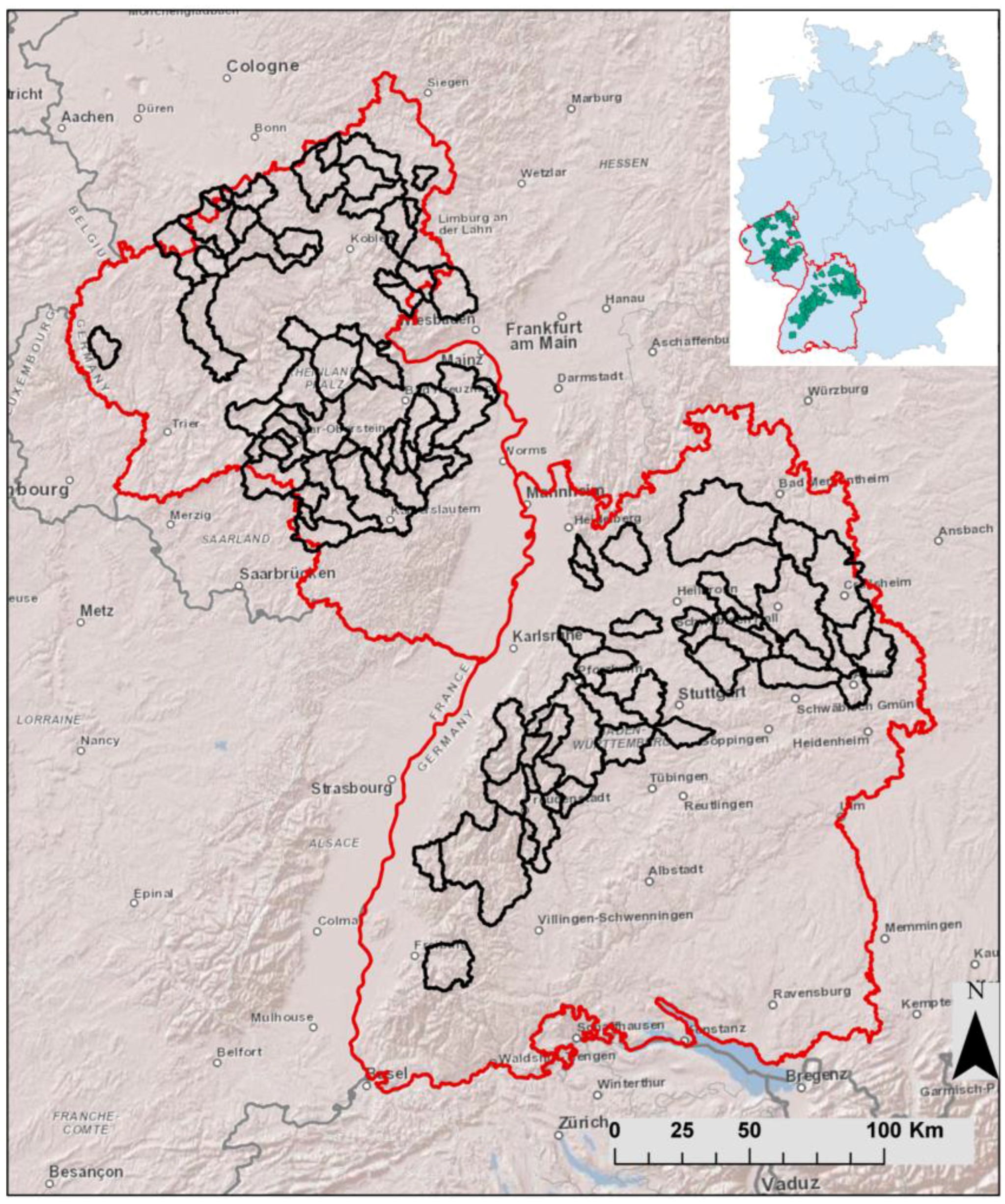Table A1 lists important characteristics of all catchments in the study area.

2.2. Data

For the model application, hourly runoff, areal precipitation, and temperature data for the period from January 1996 or January 1997 to December 2003 were used. These time series cover a wide range of diverse annual or seasonal precipitation and runoff events.

Areal precipitation and air temperature was calculated for catchments in Rhineland-Palatinate with “InterMet” [24], which interpolates meteorological data using the kriging technique. InterMet takes into account data from about 200 rain gauges, along with meteorological data, prevailing atmospheric conditions, orography, and satellite and radar data. For catchments in Baden-Württemberg areal precipitation and air temperature were calculated with the interpolation routine of the water balance model LARSIM (Large Area Runoff Simulation Model [25]). The conversion of measurements to subareas is done by a modified inverse distance method with consideration of altitude’s dependency of the temperature. The two interpolation methods for areal precipitation may have marginal effects on the calibration and therefore on the results. However, in our study, no effects were visible. Potential evaporation was calculated with Hamon’s equation [26].

The typical spatial extent of rainfall fields is in the range of most of the catchments. However, in summer, convective rainfall events may affect only parts of the catchments. Snow events occur in the study area. However, they are of minor importance since they are limited in amount, not prolonged, and irregular. Snow processes are thus not considered in the modeling exercise.

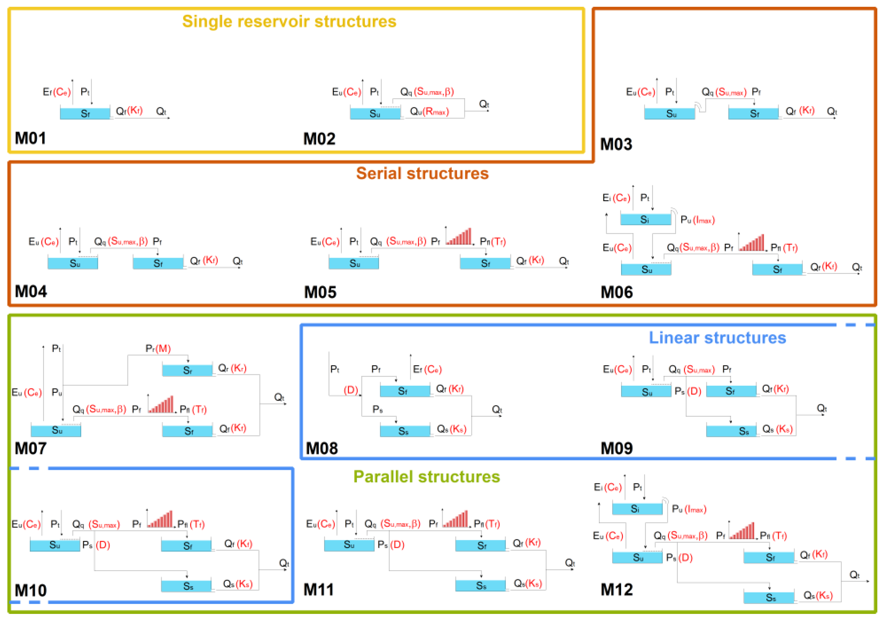
2.3. Methods

2.3.1. Calibration

For all catchments, we use eight years of hourly rainfall and runoff data. The warm-up period of the calibration consists of the first year of the data period (1996). Following a split-sample approach [27], the remaining range (1997–2003) is subdivided into a calibration period and a validation period of equal length.

We use 12 lumped conceptual model structures constructed within the SUPERFLEX modeling framework [10]. The structures are proposed by Fenicia et al. [17] for catchments in Luxemburg, and they are also used by van Esse et al. [16] for French catchments. Since all model structures are lumped, they provide physically plausible descriptions of the catchment-scale response, but the behavior of different runoff mechanisms cannot be allocated to different areas within the catchment [17].

The model structures include serial, linear, and parallel model structures with different numbers of reservoirs and parameters, thus covering a broad range of conceptual model complexities (Figure 2). M01 represents the simplest hydrological model with one nonlinear reservoir and M02 an extended single reservoir with a power function. M03 to M05 comprise two reservoirs as serial structures, representing an unsaturated and a storage reservoir. Differences are in the connection of the reservoirs: as an overflow (M03) or as a power function of the storage (M04 and M05) and including a transfer function between the reservoirs of M05. M06 is similar to M05 but with an additional interception reservoir before the unsaturated reservoir. M07 to M12 comprise two to four reservoirs in parallel arrangements. M07 has a riparian zone reservoir, which receives a constant fraction of precipitation. M08 is a simple parallel structure where precipitation is partitioned between two linear reservoirs (slow and fast). M09 is extended by an unsaturated reservoir partitioning precipitation and M10 includes an unsaturated reservoir and a transfer function. M11 is based on M10 but with an additional power function splitting the outflow of the unsaturated reservoir. For M12 is like M11 with the inclusion of an interception reservoir [17]. The number of parameters varies between two for the simplest model structure M01 to eight for model structure M12 (Figure 2). Please note that there is no linear increase in complexity from structure M01 to structure M12. Table 1 lists the ranges of all parameters.

Figure 2. Model structures, adapted from Fenicia et al. [17]. D: partition between fast and slow reservoir; E_f (Ce): actual evaporation; E_u (Ce): unsaturated evaporation; I = interception; K: storage coefficient; P: precipitation; Q: discharge; S: storage; Su_max: storage; β: power function; f = fast; r = riparian; s = slow; t = total; u = unsaturated.

Table 1. Parameter ranges of the 12 model structures. All parameters, except D and M, are converted to a logarithmic value for calibration.

Parameter	Minimum	Maximum
Ce (-)	0.01	30
D (-)	0	1
Imax (mm)	0.000001	20
Kf (1/d)	0.0000001	1
Kr (1/d)	0.00001	1
Ks (1/d)	0.0000001	1
M (-)	0	0.3
Rmax (mm/day)	0.001	30
Sumax (mm)	0.1	0.000001
Tf (d)	1	500
β (-)	0.001	50

The calibration was similar in van Esse et al. [16], except for the fact that the parameter α at the outflow of the fast reservoir of models 1, 3, 4, 5, 6, and 7 was set to 2, corresponding to a “Dupuit–Boussinesq aquifer” [28]. Van Esse et al. [16] describe this parameter as far less effective than parameter β. Parameter α showed only a marginal effect for catchments in our study area as well. With a constant parameter α, we achieve better simulations with a reduced number of calibrated parameters.

The objective function for calibration is based on a weighted least squares approach, assuming independent Gaussian error with zero mean and standard deviation linearly proportional to the modeled discharge [29]. Optimization was carried out through a quasi-Newton method with 30 multi-starts randomly selected across the parameter space.

We calibrated 12 model structures for each of the 99 catchments. Each of these 1188 models consists of a specific structure combined with a parameter set and catchment information.

2.3.2. Model Evaluation: Identification of Acceptable Models

The large scatter of signature indices for several models requires the identification of acceptable models for further analysis. The identification of acceptable models is based on thresholds of two performance measures: a combination of four signature indices derived from the Flow Duration Curve (FDC) [23] and the Nash–Sutcliffe Efficiency (NSE) [30].

The FDC represents the relationship between magnitude and exceedance probability of runoff for a single catchment. Therefore, it is a key signature of runoff variability and can be used for model evaluation and comparison [31,32,33]. Yilmaz et al. [32] developed so-called signature indices, which represent specific parts of an FDC and express the percentage biases between observed values and simulated values proportional to the observed FDC. Ley et al. [23] proposed four signature indices to examine the influence of specific aspects of the hydrograph on model performance: extreme high runoff (FHV), medium runoff (FMV), mid-slope (FMS), and low flow (FLV) (Figure 3). These four signature indices take into account the whole FDC and therefore the entire hydrograph.

Figure 3. Meaning and position of the four signature indices derived from the FDC [23]. (Copyright permission from IWA Publishing: Ley, R.; Hellebrand, H.; Casper, M.C.; Fenicia, F. Comparing classical performance measures with signature indices derived from flow duration curves to asses model structures as tools for catchment classification. Hydrol. Res. 2016, 47, 1–14.)

To evaluate model performance based on the values of the four signature indices, the absolute values of these indices are summed into one value: S_SI (Equation (1)). Because the sum of percentages as absolute values of biases can lead to misunderstandings, we set S_SI as dimensionless:

$${\mathrm{S}}_{\text{SI}}= \left|FHV\right|+\left|FMV\right|+\left|FMS\right|+\left|FLV\right|.$$

(1)

The addition of the absolute values of the signature indices considers all parts of the FDC equally. The absolute values indicate that whether the FDC is over- or underestimated is irrelevant. The values of S_SI range between zero (perfect fit) and infinity (no fit).

As the FDC does not reflect information on timing of the flow, we use the NSE (Equation (2)) to avoid recognizing models with large timing errors but an acceptable FDC by chance.

$$\text{NSE}= 1-\frac{{{\displaystyle \sum }}_{i=1}^n {\left( q_{obs}\left(i\right)-q_{sim}\left(i\right) \right)}^2}{{{\displaystyle \sum }}_{i=1}^n {\left( q_{obs}\left(i\right)-\overline{q_{obs}} \right)}^2},$$

(2)

where q_obs represents observed runoff, q_sim represents simulated runoff, the overbar denotes the mean, and n is the length of the time series. The NSE is a common normalized measure to evaluate the performance of hydrologic models and compares the mean square error of the simulated runoff to the variance of the observed runoff (Equation (2)). It ranges from minus infinity to 1, where 1 indicates a perfect fit. For characterizing streamflow performance, it is typically considered that NSE is overly sensitive to large values [34] and that the NSE is not always expedient for model evaluation and comparison [23,35].

Models are considered acceptable if S_SI is less than 70 and NSE is larger than 0.65. Models that do not fulfill these two criteria are no longer incorporated in the subsequent stages of the analysis.

The threshold values for S_SI and NSE are selected based on experience. For the NSE, the selected threshold corresponds to adequate or very good reported performance ratings for NSE according to Moriasi et al. [36], whereas Oudin et al. [37] refer to a poorly modeled catchment when the NSE is less than 0.7. The threshold of 70 for S_SI is based on visual inspections of suitable FDCs.

2.3.3. Comparing Model Performances

To separate similar from dissimilar runoff simulations, we grouped model performances by a cluster analysis with a Self-Organizing Map (SOM). Input data for the analysis are the four signature indices of each acceptable model. For catchments with more than one acceptable model, all acceptable models are included.

An SOM is an automatic data-analysis method widely applied to clustering problems and data exploration [38]. Kohonen [39] provides a detailed description of the algorithm and its properties. A SOM produces a semantic map of units, called neurons, which represent the input datasets (i.e., signature indices of models). On the map similar units are mapped closer together and dissimilar units are further apart. The semantic map also quantifies distances between units that are interpreted as borders of clusters. These groups of similar units and distances constitute clusters of models with similar signature indices. The use of SOM for cluster analysis is described in detail by Ley et al. [40,41]. For the training and visualization of the SOM we use the “SOM-Toolbox for Matlab 5” [42].

The cluster analysis groups models with similar sets of signature indices into homogenous clusters of models and therefore quantifies similarity. For each catchment we analyzed in which cluster the acceptable model results are listed. Acceptable models of one catchment in different clusters indicate discriminating results by different model structures. Multiple models of one catchment in a cluster highlight multiple model structures simulating the catchment similarly. We use the results of the cluster analysis to group the catchments:

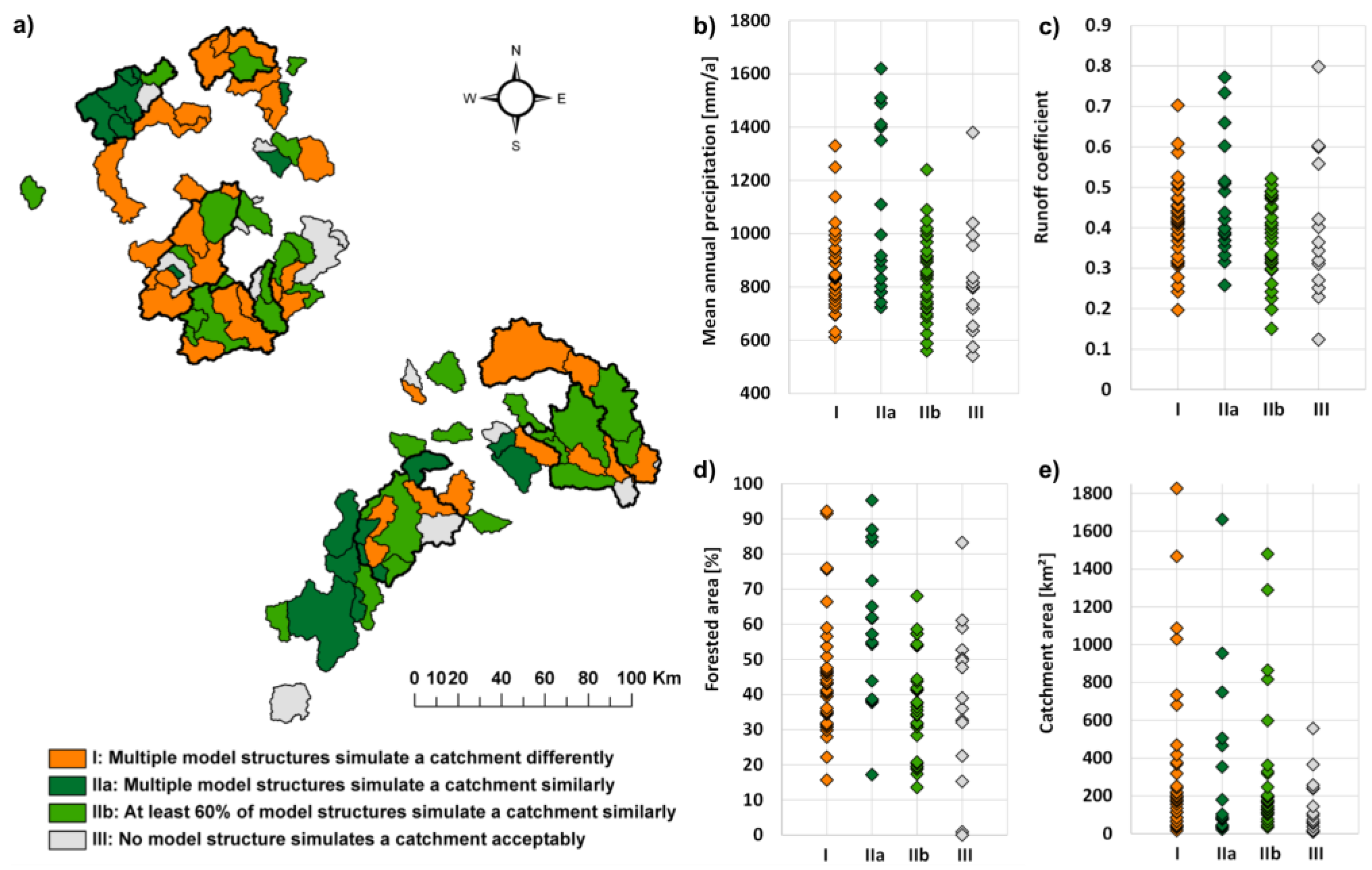
• Multiple model structures simulate a catchment differently. The identification of a best performing model is possible. The model structure can be tentatively connected to the catchment behavior. If there are catchments with only one acceptable model, they belong to this group too.
• Multiple model structures simulate the catchment similarly. Model equifinality [12,18,43] makes it difficult to connect model structure and catchment structure or behavior. Catchments of this group are further divided into:

  • catchments where all acceptable models simulate the runoff similarly; and
  • catchments where at least 60% but not all acceptable models simulate runoff similarly.
  Catchments without an acceptable model result constitute an additional group:
• No model structure simulates the catchment acceptably. All structures fail to capture catchment behavior.

2.3.4. Identification of Best Performing Models

For each catchment with acceptable models, the model with the lowest S_SI (Equation (1)) is the best performing model for this catchment. For catchments with only one acceptable model, this model is assigned as the best performing.

If models show minimal differences, an identification based on the lowest S_SI is often possible, but not very reliable. For catchments with differences of S_SI < 2.0 between models, we identify more than one best performing model.

The suitability of best performing models to represent catchment characteristics is tested by correlating them with catchment properties and catchment location.

2.3.5. Correlation with Catchment Properties

To find a link between catchment properties and model behavior, we compare catchments with the same best performing models and catchments of groups I to III with their catchment properties, neighborhoods, and nesting.

3. Results

3.1. Calibration

The calibrated models show only minor differences with reference to their performance when compared to the validation period. The mean difference between the NSE of calibrated and validated models is 0.07, with a median of 0.05. Models based on structure M03 show the highest differences, up to 0.66; most of the models show differences with a maximum of 0.2. For acceptable models, the mean difference between the NSE for the calibration and the validation period is 0.05, with a median of 0.04 and a maximum of 0.24. The highest mean differences are observed for models based on structures M01 and M08. Therefore, the analysis uses the simulated results of the calibrated models.

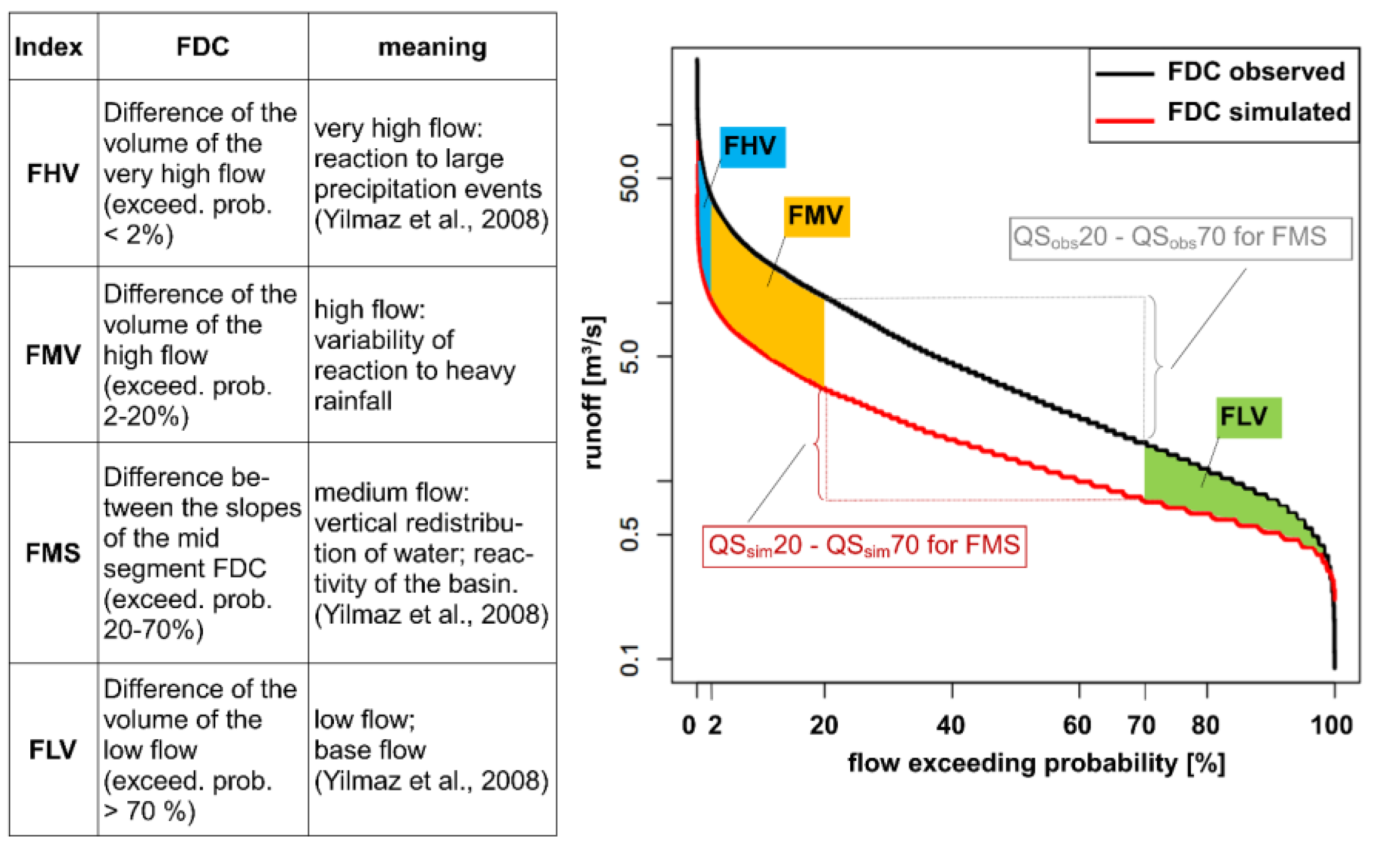
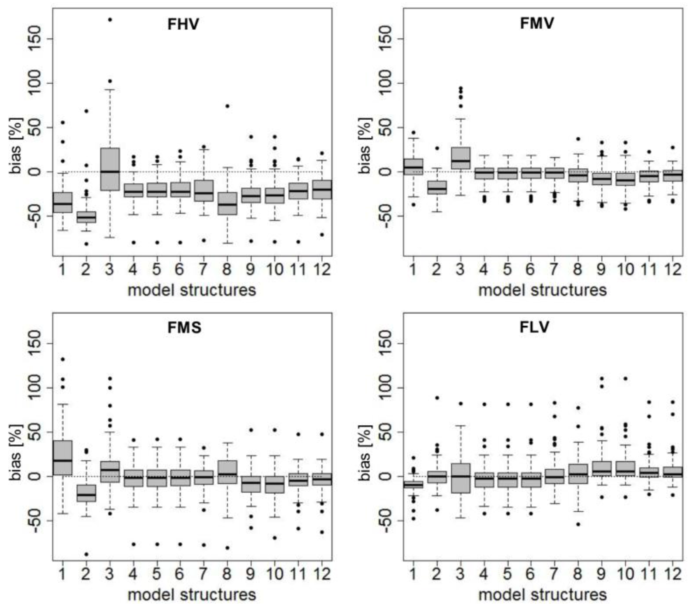
3.2. Signature Indices

The signature indices for each calibrated model show no unique model structure that represents all parts of the FDC best (Figure 4). Large biases (high values of signature indices) are predominantly found for model structures M01 to M03 and to a lesser extent for model structure M08. The biases of FHV (peak flow) show predominantly underestimations for most of the model structures. Here, only model structure M03 shows a median bias of zero, but a very high uncertainty range.

Figure 4. Box and whisker plots of the four signature indices of all models and 12 model structures. The boxplots show the interquartile ranges as boxes and the median by a black line in the middle of the box; the whiskers show the minimum and the maximum up to the 1.5 interquartile range and outliers outside the 1.5 interquartile range.

Most of the models show for the three remaining signatures a median close to zero. This indicates well performing models, except for the highest peaks. Nevertheless, from this analysis, it is not possible to clearly detect which model structure performs best.

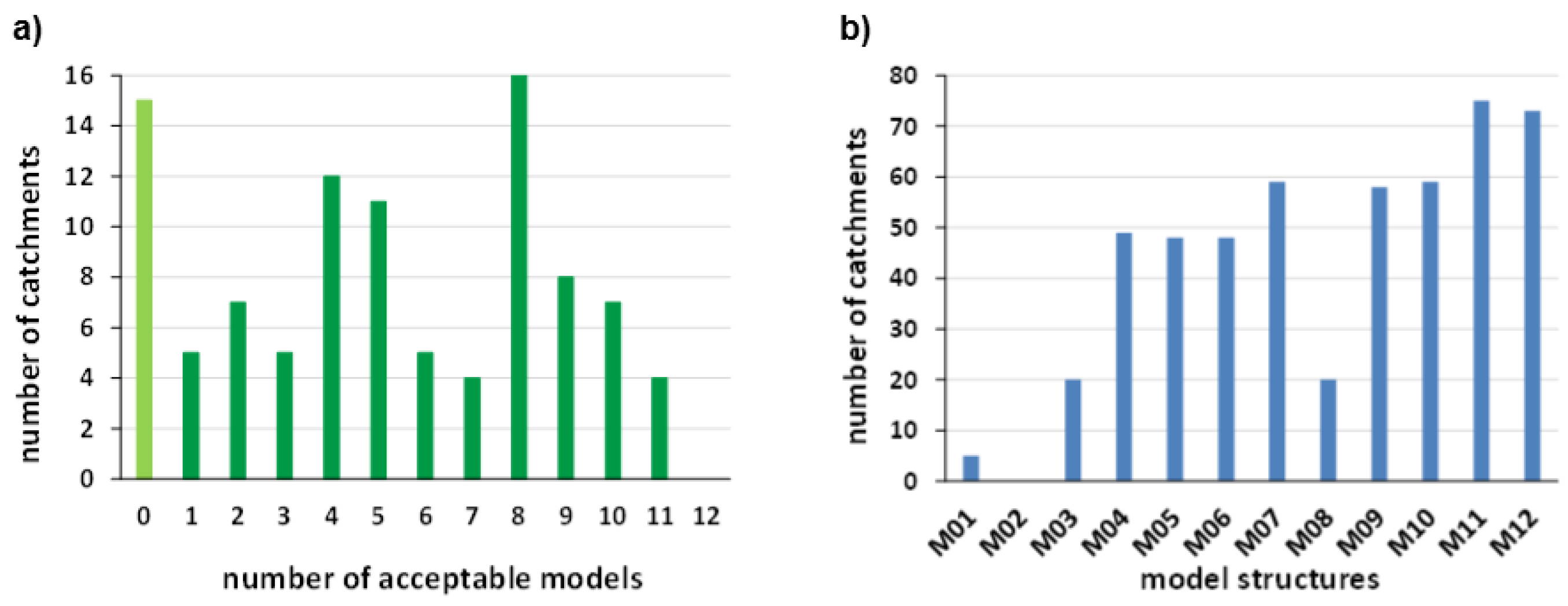
3.3. Acceptable Models

For the 99 catchments, we identified different numbers of acceptable models per catchment (Figure 5a): in total, we determined 511 acceptable models. For 15 catchments, there is no acceptable model. In addition, different model structures lead to acceptable models for a different number of catchments (Figure 5b). Model structure M02 generates no acceptable model. This indicates that model structure M02 is not suited for simulating catchments of the study area.

Figure 5. Numbers of acceptable models per catchment (a) and number of catchments where model structures M01 to M12 produce acceptable models (b).

No model structure is capable of producing an acceptable model for all catchments (Figure 5b). This shows that model structures differentiate between catchments.

3.4. Comparing Model Performances

The cluster analysis of acceptable models by their signature indices shows 14 homogenous clusters containing 13 to 78 models with similar signature indices. The analysis of models per cluster indicates that for some catchments several models have similar signature indices. Other catchments exhibit different signature indices per model. Figure 6 displays the four FDC-based signature indices of acceptable models for some catchments: the x-axis presents the signature indices; the y-axis shows the value of the indices.

Figure 6. Different sensitivities of simulated runoff to model structures for single catchments. The signature indices of a catchment are displayed and connected by a line creating a performance pattern for this model. Model structures are indicated by colors and named in the legend with the number of the model structure. (I) displays examples of catchments with differentiated patterns of signature indices; (II) performance pattern of catchments with all (a) or most (b) acceptable models with similar patterns of signature indices; and (III) catchments without an acceptable model. (I, II) show only acceptable models for these catchments; (III) shows all models of a catchment.

Based on the clusters of models with similar signature indices, we identified four groups of catchments, including a group of catchments without any acceptable model:

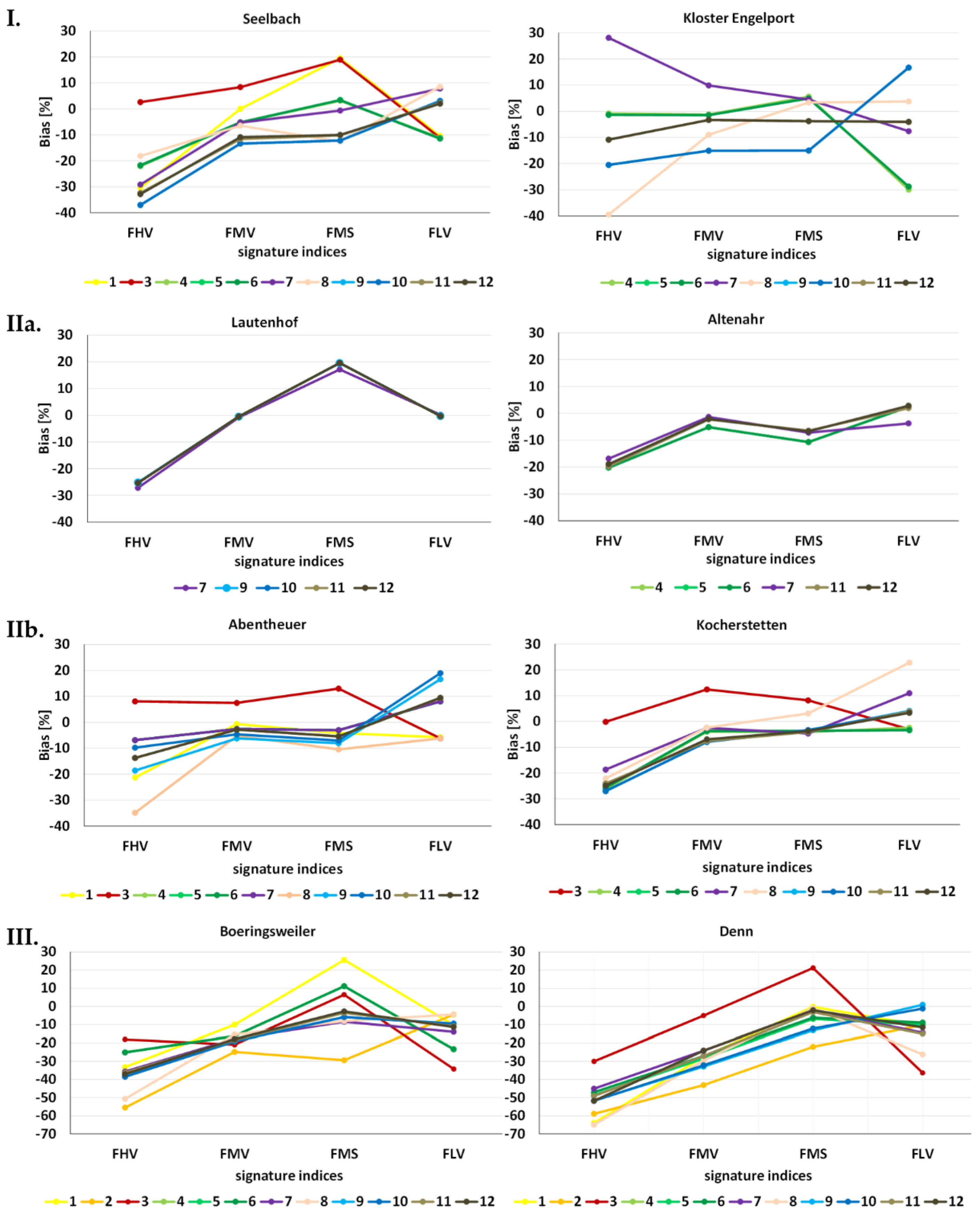
I

Multiple model structures simulate a catchment differently. The two example catchments (Figure 6I) show different patterns of signature indices.

For 30 catchments of the study area (Table A1), multiple model structures produce different simulations, even though few models show related patterns of signature indices.

Additionally, we include in this group the five catchments with only one acceptable model because of differentiated simulation results (Table A1).

IIa

All acceptable models of a catchment simulate the catchment similarly and display model equifinality [43]. This occurs for 17 catchments (Table A1); two examples are displayed in Figure 6IIa.

IIb

At least 60% of acceptable models simulate the catchment similarly (Figure 6IIb). The best performing model must not be part of the models with similar performances. This group includes 32 catchments of the study area (Table A1).

III

No model structure simulates a catchment acceptably (Figure 6III). Fifteen catchments of the study area belong to this category (Table A1), indicating conceptual, structural, or data errors [43].

Similarly performing models of a catchment (group IIa and IIb) are based on different model structures. Nearly all possible compositions of model structures occur as similarly performing models of a catchment. No model structure shows similar performance in all cases of acceptability.

Model structures with relatively seldom accepted models (i.e., model structures M01, M03, and M08) often show different patterns of signature indices than the other model structures, e.g., models M01 and M03 for catchment “Seelbach” (Figure 6I), “Abentheuer” and “Kocherstetten” (both Figure 6IIb). Model structures M01 and M08 are the only structures without a separate unsaturated reservoir and model structure M03 is the only structure in this study with a threshold function rather than a power function as outflow from the unsaturated reservoir. The remaining structures result in many acceptable models. These structures include serial, linear, and parallel structures with two to four reservoirs and four to eight parameters.

The spatial distribution of the catchments of categories I to III show no spatial correlation, neither for neighbored nor for nested catchments (Figure 7a). Furthermore, no clear correlation can be identified between these groups of catchments and catchment properties (Figure 7b–e). Only catchments with similar patterns of signature indices for acceptable models (Figure 7b, c, dark green) seem to have mean annual precipitation more than 700 mm/year and high runoff coefficients. However, there are many catchments with these properties in all groups, too.

Figure 7. Spatial distribution of catchments with similar or different patterns of signature indices (a). Borders of large catchments with several upstream catchments are marked with a bold line. Please note, nested catchments are sorted by size: only the headwater catchments are displayed completely. (b–e) display catchment properties of catchments in categories I to III.

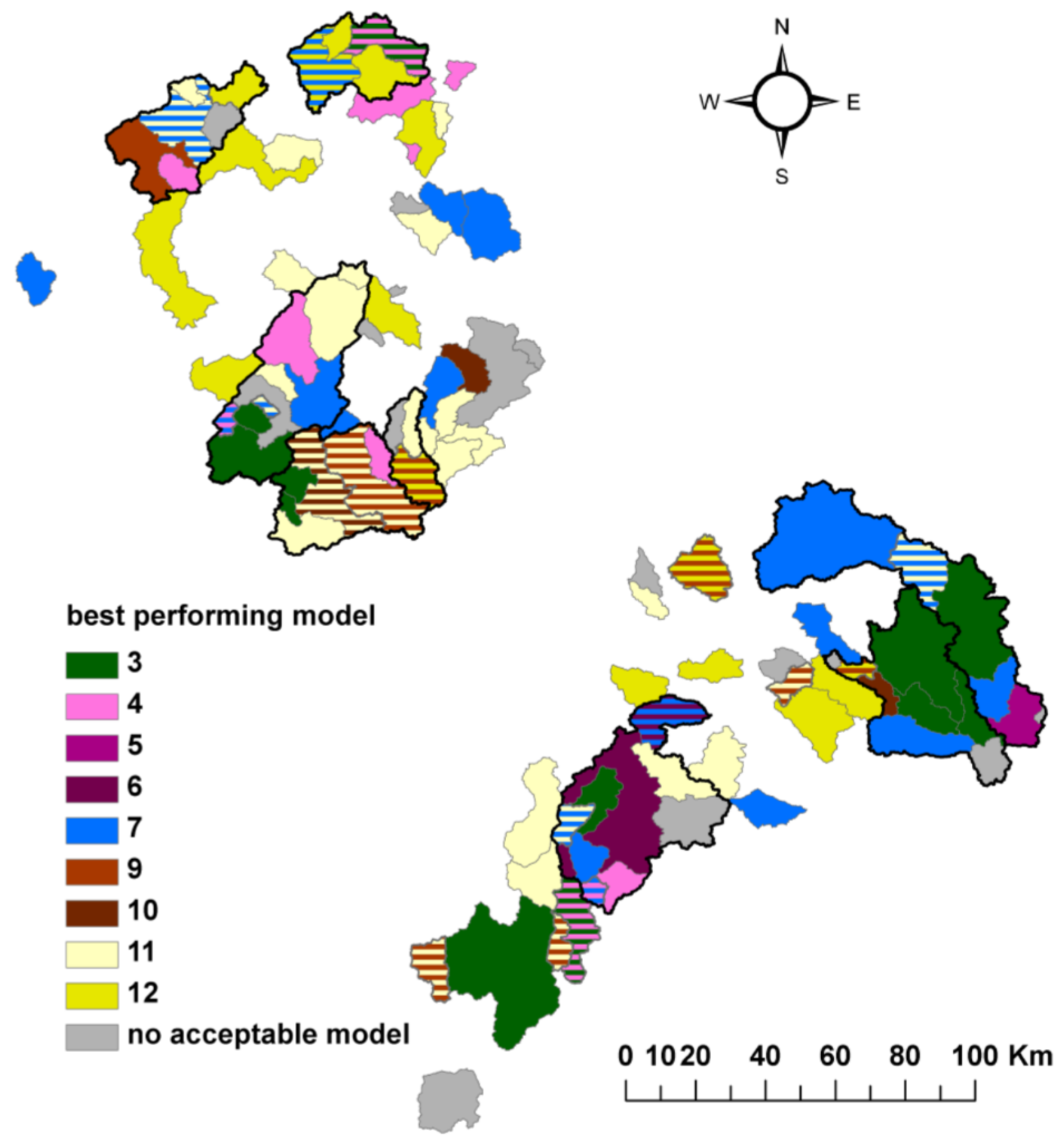
3.5. Best Performing Models

For several catchments with similar signature indices for different models, an identification based on the lowest S_SI is possible but not reliable. Therefore, all models with only minor differences of performance to the lowest S_SI (differences < 2.0) are regarded as best performing. Hence, we identify more than one best performing model for 18 catchments (Table A1). Most of these 18 catchments belong to categories IIa and IIb. Five catchments of category I show similar signature indices. Models with similar patterns of signature indices are not necessarily the best performing models of the catchment. For example, for catchment “Kocherstetten” (Figure 6IIb, on the right), the model based on structure M03 is the best performing model with an S_SI of 24 while the S_SI of other similar models are about 36.

3.6. Correlations with Catchment Properties

Figure 8 shows the spatial distribution of catchments with equal best performing models (Table A1). Catchments with more than one best performing model are striped in the color of their two best performing models. Spatial proximity is not a good predictor of the best performing model. Catchments with a best performing model are distributed throughout the study area. Even neighbored or nested catchments often have different best performing models.

Figure 8. Spatial distribution of catchments with equal best performing models. Catchments with two best performing models are striped in the color of both model structures. Please note that nested catchments are sorted by size: only the headwater catchments are displayed completely. Borders of large catchments with several upstream catchments are marked with a bold line.

Figure 9 illustrates the relationship between best performing models and mean annual precipitation, mean runoff coefficient, land use as a percentage of forested area, and catchment size. Only a few correspondences between groups of similar best performing models can be found: Model structure M03 seems to perform less well for catchments with a mean annual precipitation below 800 mm/year and low runoff coefficients, and model structure M04 seems to work well for small catchments with an area below 300 km². However, there are no clear correlations between best performing models and catchment properties like runoff characteristics, climate, land use, or catchment size.

Figure 9. Catchment characteristics of catchments sorted by the best performing model structures M01 to M12 and catchments without an acceptable model (“Model structure” 0): (a) mean annual precipitation; (b) mean runoff coefficient; (c) percentage of forested area; and (d) catchment size.

4. Discussion

The evaluation of 12 model structures on 99 catchments in Germany indicated that catchments can be classified into three categories: (I) catchments where several model structures perform differently and a best performing model structure can be identified; (II) catchments where several model structures perform similarly; and (III) catchments without well performing models. The first two classes reflect the different points of view on the general applicability of hydrological models, where the first class represents the perception that different models are appropriate in different regions, as shown in some studies e.g., [15,16]. The second class represents the perception of “equifinality” of model structures [18], which was documented in several applications too [12,14]. In our study, groups of similar performing models are made up of different combinations of model structures and nearly every possible combination of model structures does occur. The most complex models (M07, M11, or M12) do not contribute to all groups of models with similar performance. Our results reconcile these two perspectives, showing that, depending on the catchment, different results may be obtained.

We then attempted to explain why the relative ranking of various models depends on the catchment, based on proximity or catchment and climate characteristics. We found that model structure M03 seems to perform less well for catchments with a mean annual precipitation below 800 mm/year and low runoff coefficients. This model, in fact, is characterized by a threshold reservoir, and has a runoff coefficient either of 0 or of 2. We also found that model structure M04 seems to work well for small catchments with an area less than 300 km². These catchments will be on average more homogeneous than larger catchments, and can therefore be well represented by a simple structure. Models based on these structures (M03 and M04, Figure 2) are best performing for about 20% of the catchments in this study.

Apart from these conclusions, we did not find a strong correlation between best performing models and predictors such as mean annual precipitation, runoff coefficient, forested area, and catchment area. It may be that other variables not considered here, such as snow, topography, or geology, might lead to better correlations. More plausibly, there is no simple correlation between model structure and mean catchment properties at the meso-scale. Indeed, Merz and Blöschl [44], in a study on the regionalization of the HBV model parameters, did not identify a strong pattern between model parameters and various predictors.

In order to find some correlations, it may be necessary to zoom to smaller scales, such as grid elements or hydrologic response units (HRUs). Other studies have shown that these scales may be appropriate for finding suitable correlations between model structure and parameters to catchment properties [45,46].

The 12 model structures of this study do not cover all possible model structures, but a relatively broad range of complexities and a priori model hypotheses [17]. Van Esse et al. [16] showed their applicability to a wide range of catchments in France. In our study, except for structure M02, all model structures are able to simulate runoff acceptably and are able to differentiate between catchments. Additional model structures may change the division of catchments between the described groups. Therefore, the findings of this study are valid only for the used model structures and catchments. Besides these limitations, the study illustrates the different catchment characteristics in relation to conceptual models.

Dependent on the aim of model usage, differentiating catchments with or without acceptable models or equifinality may be a crucial factor. The comparison of different models remains advantageous if the objective is to improve model predictions. Lumped conceptual models are able to produce a good runoff prediction. If the modeling objective is merely the simulation of streamflow, and model realism is not an objective, the presence of model equifinality is irrelevant. If, however, model realism is an important objective, model equifinality would ideally be avoided. The identification of reasons for model equifinality of single catchments would be a step towards a better understanding of model and catchment functioning.

The connection between lumped models and real processes becomes more difficult as the scale of application increases. Large-scale processes represented in lumped models lose a direct correspondence with observations, which are usually available only at small scales. Therefore, it becomes difficult to determine a clear correspondence between processes and lumped conceptual model structures.

5. Conclusions

In this study, we calibrated 12 conceptual models on 99 catchments in Germany. The calibration was based on weighed least squares, and model performance was assessed based on the Nash–Sutcliffe efficiency and signature indices based on FDC.

Our results indicate that a classification of catchments by model structures is possible:

• For about 15% of the catchments, no model had a suitable performance, which indicates model structural errors or data errors.
• For about 50% of the catchments, large parts of the models display a similar performance and thus demonstrate strong equifinality. About 35% of the catchments show no strong equifinality.
• Most of the catchments can be classified by a clear best performing model, which indicates that models may perform differently in different regions.

We did not find significant correlations between groups of same best performing models or catchments with/without model equifinality and predictors such as mean annual precipitation, runoff coefficient, forested area, and catchment area. It might be possible that other catchment or climate characteristics would have led to better correlations. Nevertheless, we support the hypothesis that at this scale of application, it may be difficult to find relationships between model structure and parameters of lumped models and climate or catchment characteristics.

The fact that there are no predictable patterns of well performing models indicates that a priori model selection cannot be easily justified. Thus, our results support the conclusion that model selection should be done a posteriori, based on comparisons between models.

References

- McDonnell, J.J.; Woods, R. On the need for catchment classification. J. Hydrol. 2004, 299, 2–3. [Google Scholar] [CrossRef]
- Gupta, H.V.; Perrin, C.; Blöschl, G.; Montanari, A.; Kumar, R.; Clark, M.; Andreassian, V. Large-sample hydrology: A need to balance depth with breadth. Hydrol. Earth Syst. Sci. 2014, 18, 463–477. [Google Scholar] [CrossRef]
- Bárdossy, A. Calibration of hydrological model parameters for ungauged catchments. Hydrol. Earth Syst. Sci. 2007, 11, 703–710. [Google Scholar] [CrossRef]
- Clark, M.P.; Slater, A.G.; Rupp, D.E.; Woods, R.A.; Jasper, A.V.; Gupta, H.V.; Wagener, T.; Hay, L.E. Framework for Understanding Structural Errors (FUSE): A modular framework to diagnose differences between hydrological models. Water Resour. Res. 2008. [Google Scholar] [CrossRef]
- Hrachowitz, M.; Savenije, H.H.G.; Blöschl, G.; McDonnell, J.J.; Sivapalan, M.; Pomeroy, J.W.; Arheimer, B.; Blume, T.; Clark, M.P.; Ehret, U.; et al. A decade of Predictions in Ungauged Basins (PUB)–A review. Hydrol. Sci. J. 2013, 58, 1–58. [Google Scholar] [CrossRef]
- Coxon, G.; Freer, J.; Wagener, T.; Odoni, N.A.; Clark, M. Diagnostic evaluation of multiple hypotheses of hydrological behaviour in a limits-of-acceptability framework for 24 UK catchments. Hydrol. Process. 2014, 28, 6135–6150. [Google Scholar] [CrossRef]
- McDonnell, J.J. Where does water go when it rains? Moving beyond the variable source area concept of rain fall-runoff response. Hydrol. Process. 2003, 17, 1869–1875. [Google Scholar] [CrossRef]
- Savenije, H.H.G. HESS opinions “The art of hydrology”. Hydrol. Earth Syst. Sci. 2009, 13, 157–161. [Google Scholar] [CrossRef]
- Fenicia, F.; McDonnell, J.J.; Savenije, H.H.G. Learning from model improvement: On the contribution of complementary data to process understanding. Water Resour. Res. 2008. [Google Scholar] [CrossRef]
- Fenicia, F.; Kavetski, D.; Savenije, H.H.G. Elements of a flexible approach for conceptual hydrological modeling: 1. Motivation and theoretical development. Water Resour. Res. 2011. [Google Scholar] [CrossRef]
- Van Dijk, A.I.J.M. Selection of an appropriately simple storm runoff model. Hydrol. Earth Syst. Sci. 2010, 14, 447–458. [Google Scholar] [CrossRef]
- Perrin, C.; Michel, C.; Anréassian, V. Does a large number of parameters enhance model performance? Comparative assessment of common catchment model structures on 429 catchments. J. Hydrol. 2001, 242, 275–301. [Google Scholar] [CrossRef]
- Staudinger, M.; Stahl, K.; Seibert, J.; Clark, M.P.; Tallaksen, L.M. Comparison of hydrological model structures based on recession an low flow simulations. Hydrol. Earth Syst. Sci. 2011, 15, 3447–3459. [Google Scholar] [CrossRef]
- Lee, H.; McIntyre, N.; Wheater, H.; Young, A. Selection of conceptual models for regionalisation of the rainfall-runoff relationship. J. Hydrol. 2005, 312, 125–147. [Google Scholar] [CrossRef]
- Wagener, T.; McIntyre, N. Hydrological catchment classification using a data-based mechanistic strategy. In System Identification, Environmental Modelling, and Control System Design; Springer: London, UK, 2012. [Google Scholar]
- Van Esse, W.R.; Perrin, C.; Booij, M.J.; Augutsijen, D.C.M.; Fenicia, F.; Lobligeois, F. The influence of conceptual model structure on model performance: A comparative study for 237 French catchments. Hydrol. Earth Syst. Sci. 2013, 17, 4227–4239. [Google Scholar] [CrossRef]
- Fenicia, F.; Kavetski, D.; Savenije, H.H.G.; Clark, M.P.; Schoups, G.; Pfister, L.; Freer, J. Catchment properties, function, and conceptual model representation: Is there a correspondence? Hydrol. Process. 2014, 28, 2451–2467. [Google Scholar] [CrossRef]
- Beven, K. Prophecy, reality and uncertainty in distributed hydrological modelling. Adv. Water Resour. 1993, 16, 41–51. [Google Scholar] [CrossRef]
- Beven, K.; Freer, J. Equifinality, data assimilation and uncertainty estimation in mechanistic modelling of complex environmental systems using the GLUE methodology. J. Hydrol. 2001, 249, 11–29. [Google Scholar] [CrossRef]
- Buytaert, W.; Beven, K. Models as multiple working hypotheses: Hydrological simulation of tropical alpine wetlands. Hydrol. Process. 2011, 25, 1784–1799. [Google Scholar] [CrossRef]
- Clark, M.P.; Kavetski, D.; Fenicia, F. Pursuing the method of multiple working hypotheses for hydrological modeling. Water Resour. Res. 2011. [Google Scholar] [CrossRef]
- Gupta, H.V.; Wagener, T.; Liu, Y. Reconciling theory with observations: Elements of a diagnostic approach to model evaluation. Hydrol. Process. 2008, 22, 3802–3813. [Google Scholar] [CrossRef]
- Ley, R.; Hellebrand, H.; Casper, M.C.; Fenicia, F. Comparing classical performance measures with signature indices derived from flow duration curves to asses model structures as tools for catchment classification. Hydrol. Res. 2016, 47, 1–14. [Google Scholar]
- Gerlach, N. Intermet interpolation meteorologischer grössen. In Niederschlag-Abfluss-Modellierung zur Verlängerung des Vorhersagezeitraumes Operationeller Wasserstands-Und Abflussvorhersagen, Kolloquium am 27. September 2005 in Koblenz; Bundesanstalt für Gewässerkunde: Koblenz, Germany, 2006; p. 98. [Google Scholar]
- Ludwig, K.; Bremicker, M. The Water Balance Model LARSIM—Design, Content and Applications; Freiburger Schriften zur Hydrologie; Institut für Hydrologie, Universität Freiburg i. Br.: Freiburg, Germany, 2006. [Google Scholar]
- Hamon, W.R. Estimating potential evapotranspiration. J. Hydraul. Div. ASCE 1961, 87, 107–120. [Google Scholar]
- Klemeš, V. Operational testing of hydrological simulation-models. Hydrol. Sci. J. 1986, 13, 13–24. [Google Scholar] [CrossRef]
- Brutsaert, W.; Nieber, J.L. Regionalized drought flow hydrographs from a mature glaciated plateau. Water Resour. Res. 1977, 13, 637–643. [Google Scholar] [CrossRef]
- Kavetski, D.; Fenicia, F. Elements of a flexible approach for conceptual hydrological modeling: 2. Application and experimental insights. Water Resour. Res. 2011. [Google Scholar] [CrossRef]
- Nash, J.E.; Sutcliffe, J.V. River flow forecasting through conceptual models part I: A discussion of principles. J. Hydrol. 1970, 10, 282–290. [Google Scholar] [CrossRef]
- Vogel, R.M.; Fennessey, N.M. Flow-duration curves. I: New interpretation and confidence intervals. J. Water Resour. Plan. Manag. 1994, 120, 485–504. [Google Scholar] [CrossRef]
- Yilmaz, K.K.; Gupta, H.V.; Wagener, T. A process-based diagnostic approach to model evaluation: Application to the NWS distributed hydrologic model. Water Resour. Res. 2008. [Google Scholar] [CrossRef]
- Westerberg, I.K.; Guerro, J.-L.; Younger, P.M.; Beven, K.J.; Seibert, J.; Halldin, S.; Freer, J.E.; Xu, C.Y. Calibration of hydrological models using flow-duration curves. Hydrol. Earth Syst. Sci. 2011, 15, 2205–2227. [Google Scholar] [CrossRef]
- Legates, D.R.; McCabe, G.J., Jr. Evaluating the use of “goodness-of-fit” measures in hydrologic and hydroclimatic model validation. Water Resour. Res. 1999, 35, 233–241. [Google Scholar] [CrossRef]
- Schaefli, B.; Gupta, H.V. Do Nash values have value? Hydrol. Process. 2007, 21, 2075–2080. [Google Scholar] [CrossRef]
- Moriasi, D.N.; Arnold, J.G.; van Liew, M.W.; Bingner, R.L.; Harmel, R.D.; Veith, T.L. Model evaluation guidelines for systematic quantification of accuracy in watershed simulations. Am. Soc. Agric. Biol. Eng. 2007, 50, 885–900. [Google Scholar]
- Oudin, L.; Andréassian, V.; Perrin, C.; Michel, C.; Moine, N.L. Spatial proximity, physical similarity, regression and ungaged catchments: A comparison of regionalization approaches based on 913 French catchments. Water Resour. Res. 2008. [Google Scholar] [CrossRef]
- Kohonen, T. Essentials of the self-organizing map. Neural Netw. 2013, 37, 52–65. [Google Scholar] [CrossRef]
- Kohonen, T. Self-Organizing Maps, 3rd ed.; Springer Series in Information Sciences; Springer-Verlag: Berlin, Germany, 2001. [Google Scholar]
- Ley, R.; Casper, M.C.; Hellebrand, H.; Merz, R. Catchment classification by runoff behaviour with self-organizing maps (SOM). Hydrol. Earth Syst. Sci. 2011, 115, 2947–2962. [Google Scholar] [CrossRef]
- Ley, R. Klassifikation von Pegel-Einzugsgebieten und Regionalisierung von Abfluss-Und Modell-Parametern unter Berücksichtigung des Abflussverhaltens, Hydroklimatischer und Physiogeografischer Gebietsmerkmale. Ph.D. Thesis, Universität Trier, Trier, Germany, 2014. [Google Scholar]
- Vesanto, J.; Alhoniemi, E. Clustering of the self-organizing map. IEEE Trans. Neural Netw. 2000, 11, 586–600. [Google Scholar] [CrossRef]
- Beven, K.J. Uncertainty in Environmental Modelling: A Manifesto for the Equifinality Thesis. In Proceedings of the international workshop on uncertainty, sensitivity and parameter estimation for multimedia environmental modelling, Rockville, MD, USA, 19–21 August 2003; pp. 103–105.
- Merz, R.; Blöschl, G. Regionalisation of catchment model parameters. J. Hydrol. 2004, 287, 95–123. [Google Scholar] [CrossRef]
- Samaniego, L.; Kumar, R.; Attinger, S. Multiscale parameter regionalization of a grid-based hydrologic model at the mesoscale. Water Resour. Res. 2010. [Google Scholar] [CrossRef]
- Fenicia, F.; Kavetski, D.; Savenije, H.H.G.; Pfister, L. From spatially variable streamflow to distributed hydrological models: Analysis of key modeling decisions. Water Resour. Res. 2016, 52, 1–36. [Google Scholar] [CrossRef]