Abstract
A hydrological ensemble prediction system is running operationally at the Royal Meteorological Institute of Belgium (RMI) for ten catchments in the Meuse basin. It makes use of the conceptual semi-distributed hydrological model SCHEME and the European Centre for Medium Range Weather Forecasts (ECMWF) ensemble prediction system (ENS). An ensemble of 51 discharge forecasts is generated daily. We investigate the improvements attained through postprocessing the discharge forecasts, using the archived ECMWF reforecasts for precipitation and other necessary meteorological variables. We use the 5-member reforecasts that have been produced since 2012, when the horizontal resolution of ENS was increased to the N320 resolution (≈30 km over Belgium). The reforecasts were issued weekly, going back 20 years, and we use a calibration window of five weeks. We use these as input to create a set of hydrological reforecasts. The implemented calibration method is an adaption of the variance inflation method. The parameters of the calibration are estimated based on the hydrological reforecasts and the observed discharge. The postprocessed forecasts are verified based on a two-and-a-half year period of data, using archived 51 member ENS forecasts. The skill is evaluated using summary scores of the ensemble mean and probabilistic scores: the Brier Score and the Continuous Ranked Probability Score (CRPS). We find that the variance inflation method gives a significant improvement in probabilistic discharge forecasts. The Brier score, which measures probabilistic skill for forecasts of discharge threshold exceedance, is improved for the entire forecast range during the hydrological summer period, and the first three days during hydrological winter. The CRPS is also significantly improved during summer, but not during winter. We conclude that it is valuable to apply the postprocessing method during hydrological summer. During winter, the method is also useful for forecasting exceedance probabilities of higher thresholds, but not for lead times beyond five days. Finally, we also note the presence of some large outliers in the postprocessed discharge forecasts, arising from the fact that the postprocessing is performed on the logarithmically transformed discharges. We suggest some ways to deal with this in the future for our operational setting.
1. Introduction
The benefit of using the results of meteorological ensemble prediction systems for hydrological purposes has been well established by now (see e.g., [1] for an extensive review). A large number of experimental and operational hydrological ensemble prediction systems (HEPS) have already been developed and tested (e.g., [2,3,4,5]). Typically, precipitation forecasts, and also forecasts of other meteorological fields, are used as input for a hydrological model to obtain hydrological ensemble predictions.
Ensemble precipitation forecasts help to take into account uncertainties in future rainfall, but the uncertainty is certainly not fully captured. The use of raw precipitation ensembles induces biases and inaccuracies to the input of a hydrological model (errors in the forcing). The initial conditions are imperfectly known or modeled. The hydrological model itself induces further model errors. These errors can be reduced by statistical postprocessing methods [4,6,7]. Such methods make use of (preferably long) sets of training data of both model forecasts and corresponding observations. This explains the need for reforecasts.
The use of postprocessed precipitation as input for hydrological ensemble forecasts has been tested [8,9]. The results show that the errors linked to hydrological modelling remain a key component to the total predictive uncertainty. Fundel and Zappa [4] have demonstrated that hydrological reforecasts allow for more skillful forecasts by compensating for forecast error induced by less accurate initializations. For a good overview and further references of postprocessing hydrological ensemble forecasts, we refer to the postprocessing intercomparison of [10]. The authors conclude that postprocessing is an important step to achieve forecasts that are unbiased, reliable, have the highest skill and accuracy possible, and that are coherent with the climatology.
Some recent work has focused on postprocessing, making use of European Centre for Medium Range Weather Forecasts (ECMWF) reforecasts [7,11]. Up to recently, these were produced on a weekly basis (Thursdays), and consisted of 5-member ensembles. Currently, ECMWF produces reforecasts on a bi-weekly basis, with 11-member ensembles.
In a recent study, Roulin and Vannitsem [7] investigated the use of various postprocessing methods based on reforecasts—both on the precipitation input ensembles and discharge forecasts produced with a simple conceptual hydrological model. The authors show that postprocessing precipitation forecasts alone does not improve the resolution of the resulting hydrological ensemble predictions. This indicates the usefulness of was postprocessing directly the hydrological ensemble predictions and the development of hydrological reforecasts.
In the present study, we build further on the work of Roulin and Vannitsem [7]. We apply a postprocessing method on our operational HEPS, which we describe further below. We apply the variance inflation method [12,13], estimating the calibration parameters using 5-member hydrological reforecasts over 20 years, and validate the method by applying the calibration to our archived 51-member hydrological discharge forecasts from 2012 to 2015.
In Section 2, we give a brief overview of the hydrological model, our hydrological ensemble prediction system, and the basin used in this study. We discuss the applied postprocessing method in Section 3, and the verification methodology in Section 4. In Section 5, we present and discuss the most important results. Finally, we present our conclusions in Section 6.
2. The Hydrological Ensemble Prediction System
2.1. The Hydrological Model
The SCHEME hydrological model was developed to simulate the water balance in the Scheldt and Meuse river basins. This model has been used in various studies, such as the impact of climate change and hydrological ensemble predictions [2].
The SCHEME model comprises a conceptual semi-distributed hydrological model, adapted from the IRMB water balance model [14] on 7 km grid cells, and a routing procedure based on the width function. The model can be considered as a transfer function for precipitation, with various conceptual reservoirs lumped over grid cells. It includes a snow layer, nine land covers with an interception layer and two soil layers per vegetation cover, two underground reservoirs (simulating aquifer and alluvial water), and a unit hydrograph for simulating surface runoff. There are ten adjustable model parameters. The routing of the flow from the grid cells to the outlet requires two further parameters.
The main input information for SCHEME is daily precipitation data; other meteorological data are used as well (temperature, air humidity, wind speed, surface solar radiation, and solar duration) to account for snow melt and evapotranspiration (Penman formulation).
Real-time precipitation data is taken from the weather radars at Wideumont and Avesnois, and automatic raingauges from the Royal Meteorological Institute of Belgium (RMI) and the Service Public de Wallonie (SPW). An update is performed once per month, when quality-controlled precipitation data from the RMI climatological network becomes available. Other meteorological data are collected from the RMI synoptic and automatic weather stations.
SCHEME gives daily river discharge output for catchments in the Meuse and Scheldt river basins. In this work, we focus on the Ourthe catchment at Tabreux, a tributary of the Meuse.
2.2. Study Basin
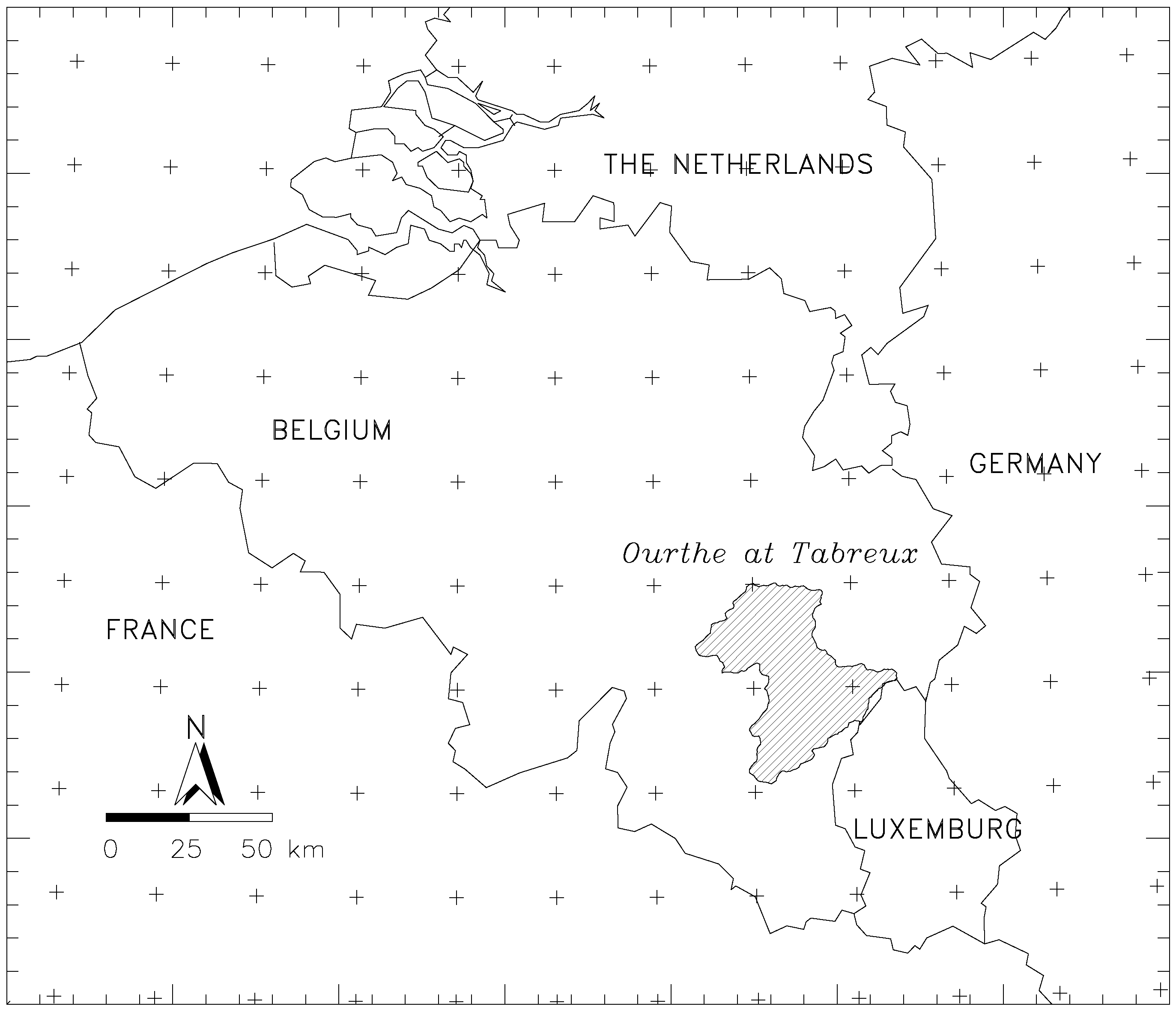
The test basin is the Ourthe basin at Tabreux, with upper part in the Ardennes region in Belgium (area 616 km, elevation 117–650 m, and mean annual rainfall 980 mm). The topography is hilly (see Figure 1), and the hydrology is dominated by surface runoff.
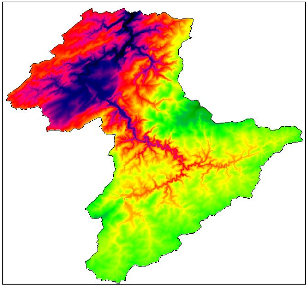
Figure 1.
Topography of the Ourthe catchment, 117–650 m.
Data from January 1990 to March 2015 are used in this study. Daily discharge data were measured at the stream gauge of Tabreux, after undergoing quality control by SPW. Precipitation data from daily pluviometric observations were interpolated to the SCHEME model grid, averaged using the method of Thiessen polygons.
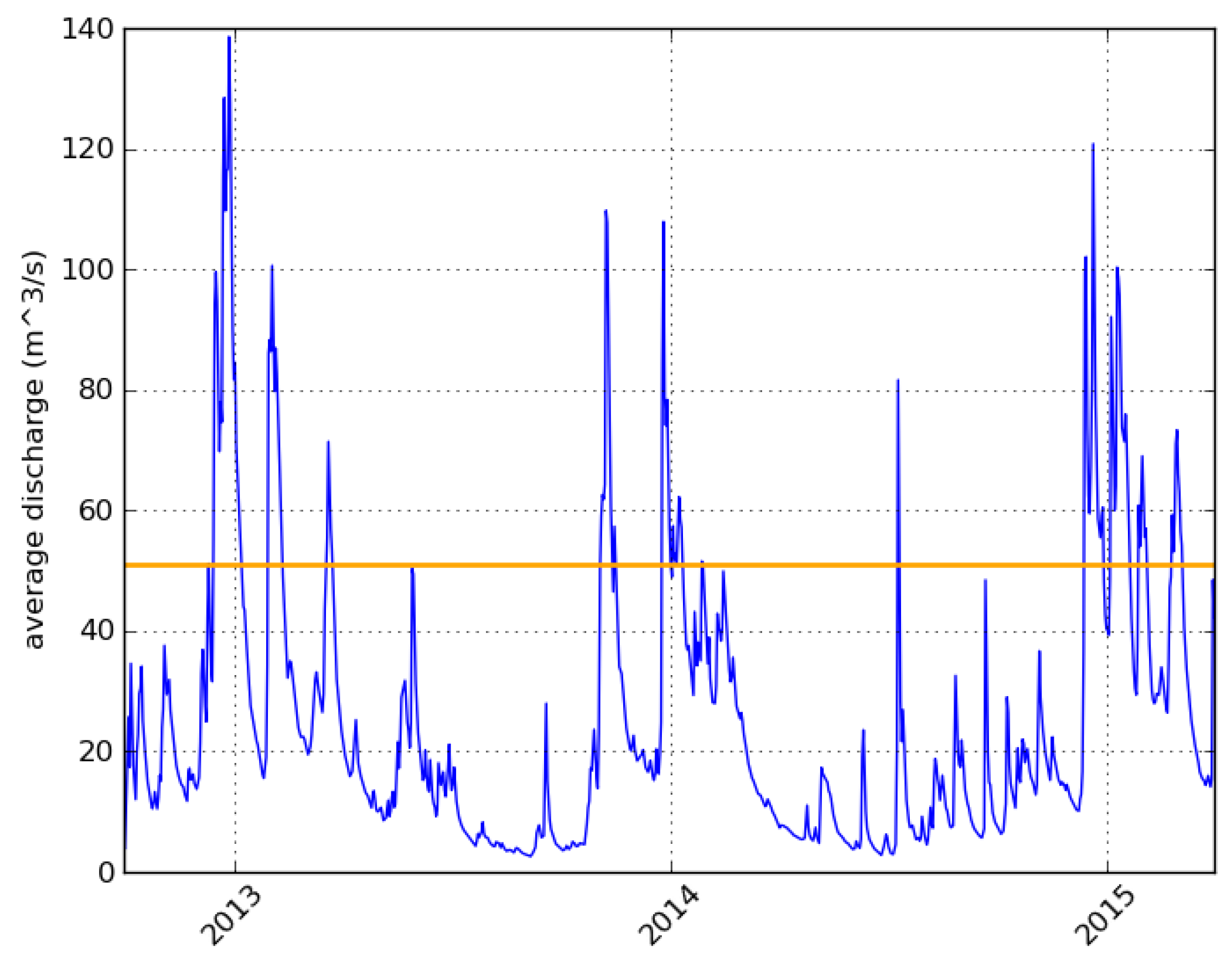
See Figure 2 for a map of the catchment, and Figure 3 for the observed discharge during the verification period.
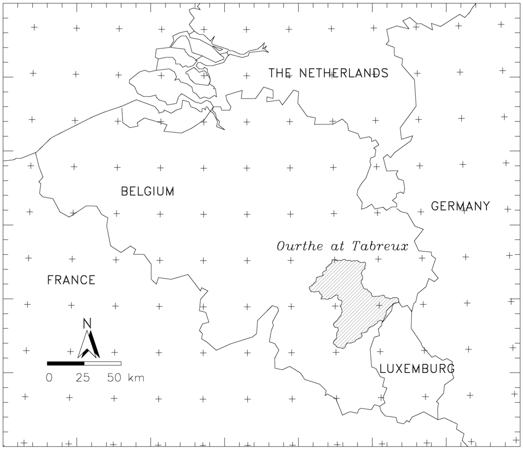
Figure 2.
Map of the Ourthe catchment. Also shown are the Ensemble Prediction System (ENS) N320 grid points.

Figure 3.
Observed average daily discharge of the Ourthe at Tabreux (blue line), and P90 threshold (orange line). The P90 threshold is the discharge that is exceeded 10% of the time during the verification period.
2.3. Operational Ensemble Forecasts
SCHEME provides the initial conditions in each grid cell at day D. It is then run in forecast mode, forced with input data from the ECMWF ensemble prediction system (ENS). We use precipitation forecasts cumulated over 24 h from 06:00 UTC to 06:00 UTC to match observations as closely as possible. These are interpolated from the ENS N320 reduced gaussian grid, with ≈30 km resolution over Belgium (see Figure 2) to the SCHEME model grid. We also use the ENS forecasts for the other meteorological input fields of SCHEME (temperature, relative humidity, solar radiation, and solar duration). Finally, a simple discharge updating procedure is applied, making use of the SPW observed discharge during the previous day, and an autoregressive error model.
Operationally, “leg A” of the ENS forecast is used: this is the first part of the ENS forecast, with a 240 h range and a ≈30 km resolution. Note that since March 2016, the ENS forecasts are available at a resolution of ≈16 km for the entire range of 15 days. Starting from initial conditions at day D (06:00 UTC) and using the 51 ensemble forecasts (issued at 00:00 UTC), results in 51 daily discharge forecasts for D+1 to D+9. The number of members with discharge greater than a threshold gives an estimate of the exceedance probability. Issuing better exceedance probabilities is one of the aims of applying a postprocessing method.
The main use of the forecasts is to issue pre-alerts for high waters at medium to long range lead times, to help support Belgian regional authorities responsible for water management. A hindcast and verification of the forecasting system was performed by [15].
3. Postprocessing
3.1. ECMWF Ensemble Prediction System and Reforecasts
For an introduction to the use of the ECMWF reforecasts, we refer to [11]. In this study, we make use of the ECMWF reforecasts produced between 20 June 2012 and 31 March 2015. The reforecasts were issued once a week. They were made available each Monday for situations starting 17 days later (Thursday) and for the past 20 years. This schedule allows for windows extending to two weeks ahead of the current week. We choose to use a calibration window of five weeks (two weeks before and two weeks after), and the full twenty years of past situations. This means that for every week, a sample of 100 ensemble forecasts is available for calibration purposes. Reforecasts are based on five-member ensembles: one control member and four perturbed members.
For verification purposes, we have access to archived ENS forecasts, issued daily at 00:00 UTC during the period from 20 June 2012 to 31 March 2015. These ensembles are composed of 1 control member and 50 perturbed members. We refer to Table 1 for a summary of the training and verification data sets.

Table 1.
Data sets.
As an example, consider the ECMWF reforecast issued on the date Thursday 25 December 2014. This reforecast contains forecast data for 20 dates: 25 December 1994, …25 December 2013. For the forecast of 27 December 2014, e.g., we calibrate the parameters based on the reforecasts issued on 11 December 2014, 18 December 2014, 25 December 2014, 1 January 2015, and 8 January 2015.
3.2. Variance Inflation
For discharge forecast postprocessing, we use the variance inflation method as adapted by [7] from [12,13]. We make use of the training data set comprised of the hydrological reforecasts (obtained using the ECMWF reforecasts, see Section 3.1) and the true observed daily discharges obtained from SPW (see Section 2.2).
The variance inflation method is based on the conditions that the climatological variance of the ensemble members should be the same as the variance of the truth and that the correlation of the ensemble members with the ensemble mean should be the same as the correlation of the truth with the ensemble mean. It also satisfies that the mean square error (MSE) of the ensemble mean is minimized and that the ensemble spread is, on average, representative of the uncertainty in the mean [12].
In the method of [7], the ensemble traces are preserved and the bias is corrected. They also apply a correction for the ensemble size, since the postprocessing parameters are calibrated on hydrological reforecasts with ensemble size , while the method is intended for ensembles with .
At time t, the ensemble member is modified following:
where is the ensemble mean and is the deviation to the mean, and where and are respectively the mean of the observations and the mean of the forecasts in the calibration dataset. The postprocessing parameters are calculated with:
where is the correlation of the observation with the ensemble mean, is the standard deviation of the observations, is the standard deviation of the ensemble mean, and is the square root of the average ensemble variance. The parameters of the calibration are estimated based on the hydrological reforecasts and corresponding true values .
According to [7], the parameters corrected for the reforecast ensemble size are given by:
where is the covariance of the true values with the reforecast ensemble mean , is the variance of the reforecast ensemble mean, and is the average of the reforecast ensemble variance.
The parameters are estimated on the logarithm of observations and of the reforecasts so that the distributions are closer to a Gaussian. Postprocessed logarithms of the discharges are exponentiated and the verification is performed in discharge units. This can give rise to distortion when the corrected discharges are transformed back, due to the non-linearity of the transformation. We will see that this does indeed cause some unrealistic effects (see Section 4 below).
4. Verification
We perform a verification study for the period June 2012 until March 2015, making use of the archived ENS forecasts and observed daily discharges during this period. For each date in the verification period, the postprocessing method is calibrated based on the reforecasts from the preceding 20 years. Note that the number of ensemble members is different: the verification is performed on the postprocessed full 51-member hydrological ensemble forecasts. See Table 1.
Our aim is to determine whether the variance inflation method is suitable for operational use in issuing exceedance probabilities for various discharge thresholds. We compare the postprocessed and raw ensemble forecasts directly with the observed discharges to check if there is an improvement.
Verification scores are also computed separately for hydrological winter (October–March) and summer (April–September) situations, due to the difference in events that typically cause high waters and flooding: mainly long periods of stratiform precipitation in winter and convective events during summer. As discussed in [15], the HEPS typically performs much better during hydrological winter.
As an additional experiment, we also perform a calibration and verification using the “reference” discharge, which is generated by forcing the SCHEME model with observed precipitation.
We focus on the probabilistic skill scores. We evaluate the skill at forecasting discharge threshold exceedance using the Brier Score, for which we consider the P90 and P80 discharge thresholds, the discharge that is exceeded 10% and 20% of the time respectively during the verification period. We also consider the Continuous Ranked Probability Score (CRPS): a score that provides an overall measure of probabilistic skill.
The Brier Score (BS) for a discrete set of probability forecasts and corresponding binary observations is given by
where is the probability assigned to the event by the forecast, and is the corresponding observation (one if the event occured, zero otherwise). The Brier Skill Score (BSS) measures the Brier score with respect to a reference: , where is the BS of the reference forecast. A perfect forecast has , while the reference forecast has .
We use the climatological frequency of threshold exceedance in the verification sample as a reference (discharge time series June 2012–March 2015). For the postprocessed forecasts, we also consider the BS of the raw ensemble forecasts as a reference, and check for improvement ().
The CRPS is defined as the integrated square difference between the cumulated forecast and observation distributions. Its deterministic limit is the mean absolute error. For its computation, we implement the expression for the CRPS as derived in [16]. The Continuous Ranked Probability Skill Score (CRPSS) measures the CRPS with respect to a reference: .
Confidence Intervals
To give an idea of the uncertainty bounds on our skill scores, we generate confidence intervals with a simple bootstrapping method.
We perform N resamplings with replacement in the set of forecast discharge and corresponding observed values (we take ). We then generate a confidence interval using the and quantiles.
The postprocessing method can be said to give a significant improvement when the BSS of the postprocessed forecast is positive with respect to the raw ensemble forecast—that is, when a BSS value of zero is outside the confidence interval.
Concerning the CRPS, we consider the significance of the improvement to the CRPSS, with the raw forecast taken as reference for the postprocessed forecast.
5. Results and Discussion
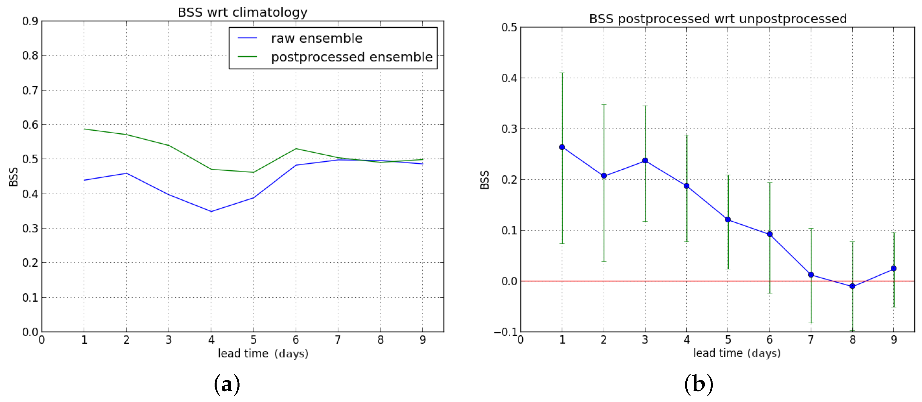
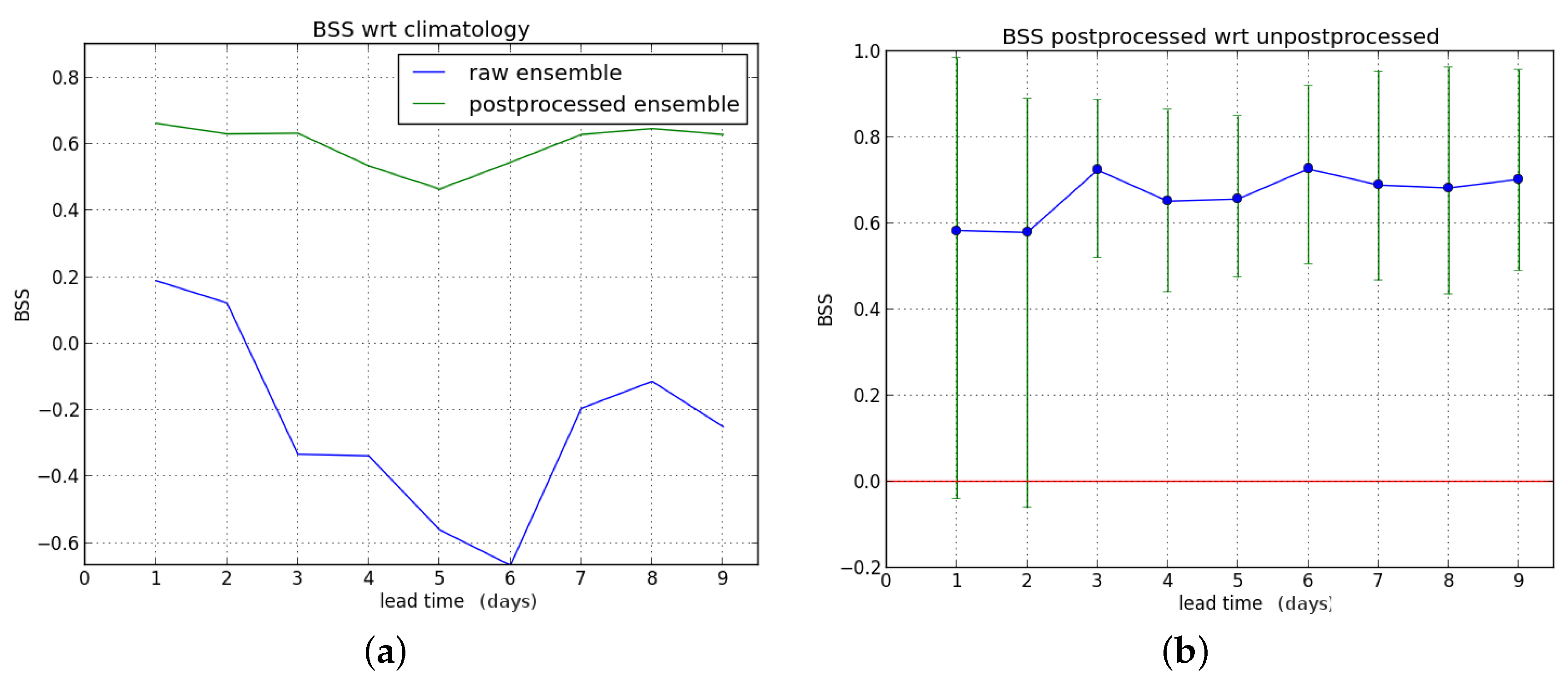
We first consider the Brier skill score (BSS) for exceedance of the P90 threshold as a function of lead time (one to nine days ahead). First, we compute the BSS of the raw and postprocessed forecasts with the sample climatology as reference, and subsequently the Brier score of the raw forecast is used as reference to compute the BSS of the postprocessed ensemble forecast.
We show the results for the entire verification period in Figure 4.
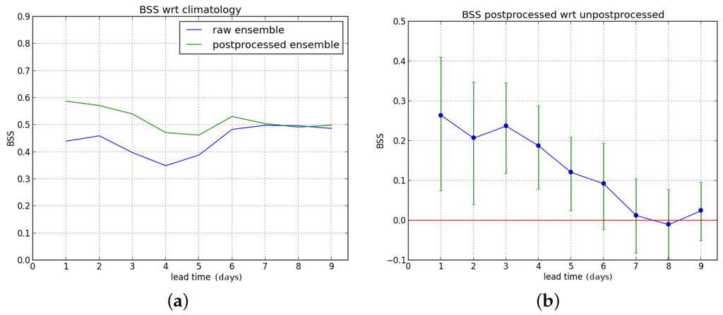
Figure 4.
Brier Skill Score (BSS) for P90 threshold during entire verification period. (a) Compared to sample climatology; (b) Improvement due to postprocessing.
The postprocessing leads to a significant improvement for lead times up to five days ahead. Starting from leadtime D+6, a BSS value of zero (no improvement) is within the confidence interval (see Figure 4b).
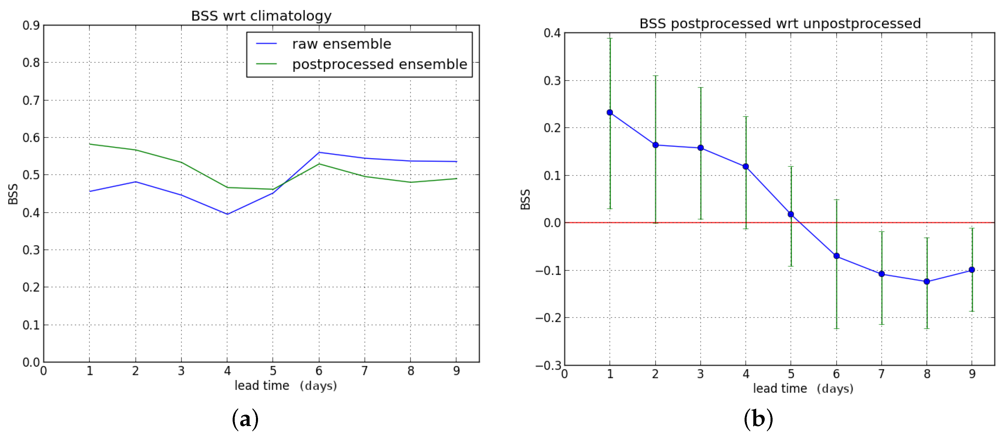
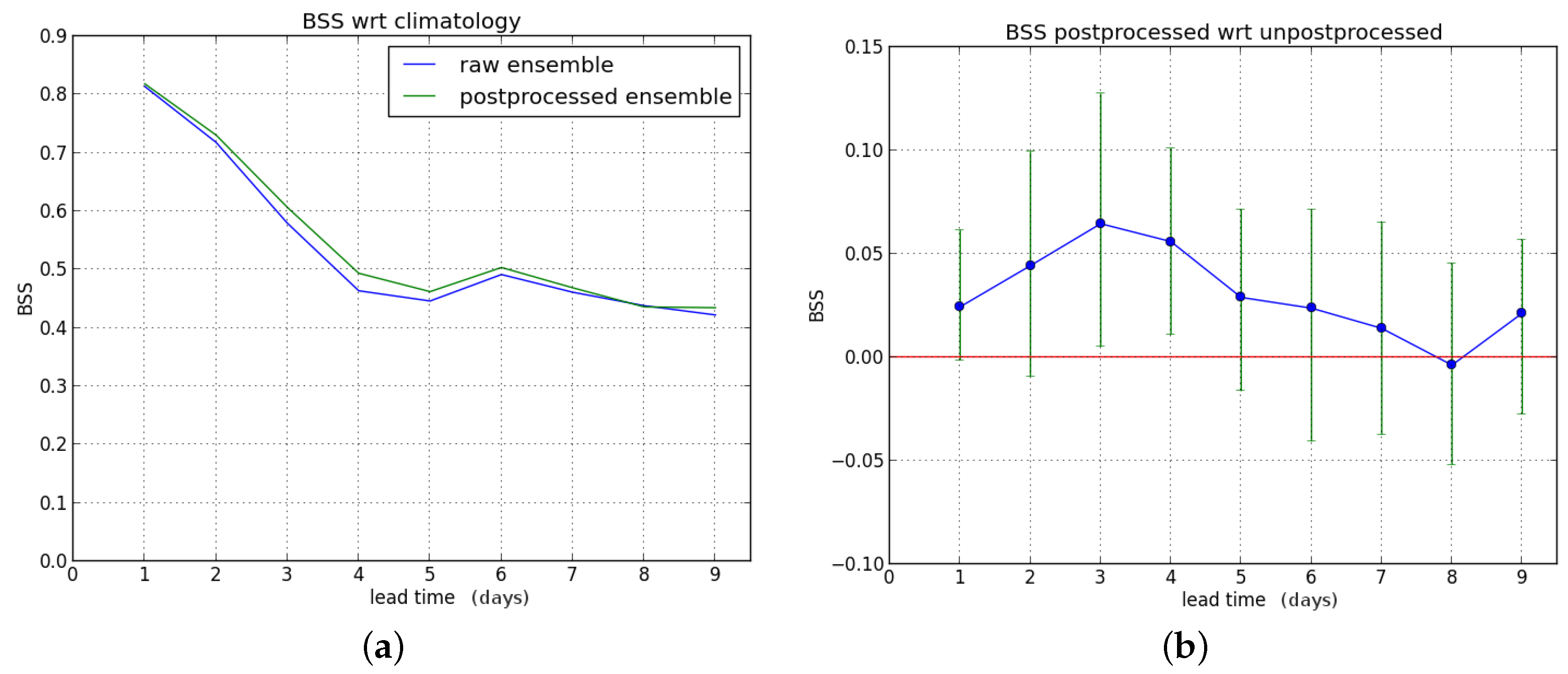
When we consider hydrological winter only, the results are given in Figure 5. Postprocessing gives an improvement for lead times up to three days ahead, but degrades the forecasts at long lead times (seven to nine days ahead).

Figure 5.
Brier Skill Score for P90 threshold during hydrological winter. (a) Compared to sample climatology; (b) Improvement due to postprocessing.
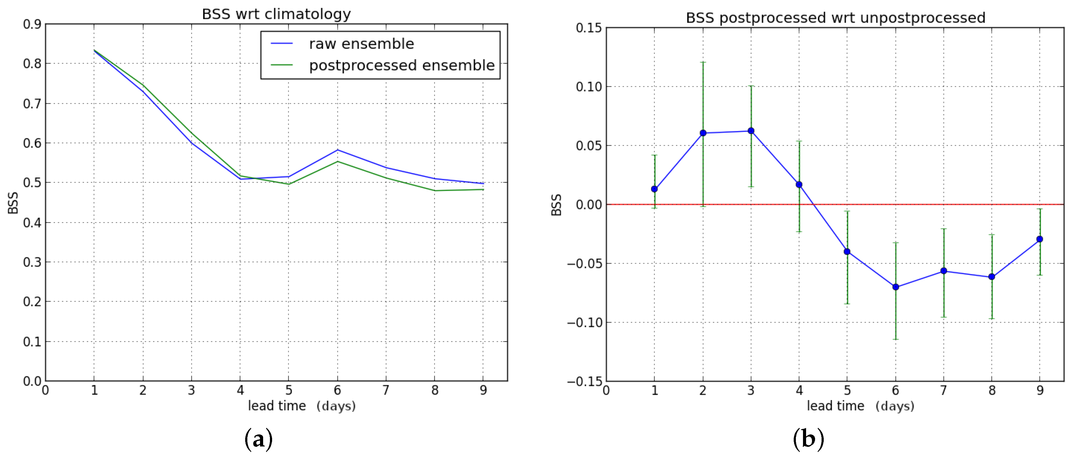
For hydrological summer, we refer to Figure 6. The postprocessing method gives a significant improvement for almost the entire forecast range. Note that there are fewer exceedance events during summer. Further examination of the data reveals that the postprocessing method mainly reduces the number of “false alarm cases”. during this period: cases where no exceedance of the P90 threshold is observed, and where the raw ensemble forcast gives a non-zero probability of exceeding the threshold, which is reduced to zero by the postprocessing. Note that we use the term loosely—the actual false alarm rate would depend on the probability threshold set for acting or not acting.
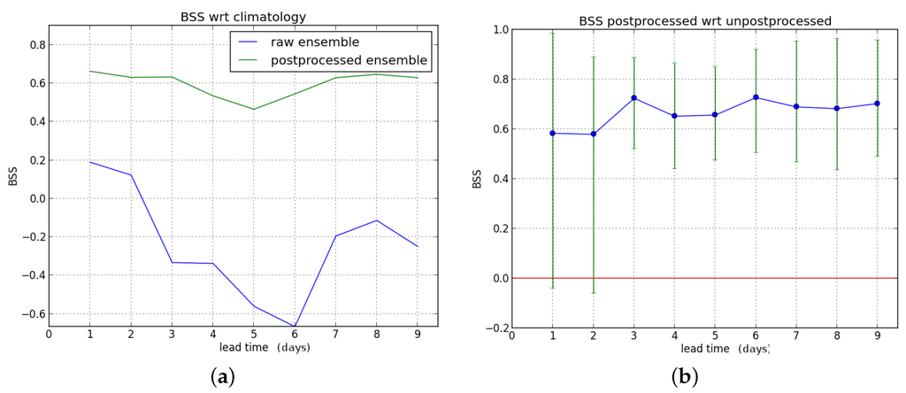
Figure 6.
Brier Skill Score for P90 threshold during hydrological summer. (a) Compared to sample climatology; (b) Improvement due to postprocessing.
We also considered the exceedance of the P80 threshold. Results (not shown here) are qualitatively similar. The only difference is that the postprocessing method gives a slightly larger improvement in BSS, significant up to six days ahead when the entire verification period is considered.
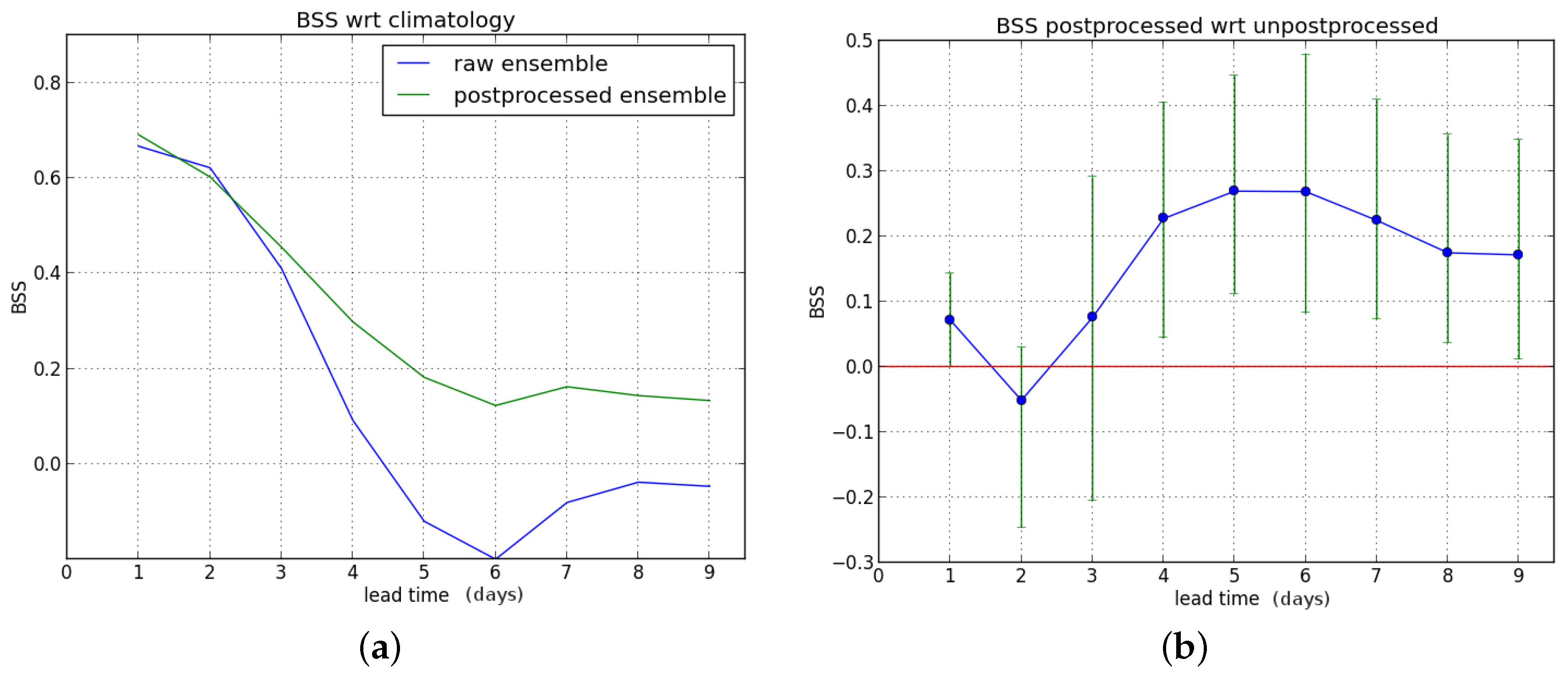
In a last experiment, we force the SCHEME model with observed precipitation and take the resulting output as the truth so that the skill of the hydrological ensemble forecast and the improvement achieved by postprocessing are evaluated in a “perfect hydrological model” setting. Results for the postprocessing with respect to this “reference discharge” are shown in Figure 7 for the entire verification period at the P90 threshold.
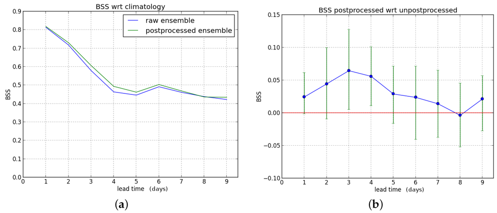
Figure 7.
Brier Skill Score for the P90 threshold. Comparison with reference discharge, entire verification period. (a) Compared to sample climatology; (b) Improvement due to postprocessing.
We see that the postprocessing gives a slight improvement in BSS over the whole forecast range, but only significantly for lead times of two and three days. Once again, results for the P80 threshold are similar, but with slightly larger improvement due to postprocessing.
For hydrological winter and summer, the results are shown in Figure 8 and Figure 9, respectively. The BSS for hydrological winter is improved during the first days and degraded from the fifth forecast day. During summer, there is an improvement beyond three days. Note that the BSS of the raw ensemble forecast becomes negative after four days; after postprocessing, there is skill during the entire forecast range. Also, comparing Figure 8 and Figure 9 to Figure 5 and Figure 6, respectively, we conclude that the postprocessing partly compensates for hydrological model errors.
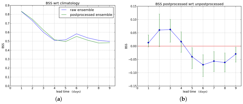
Figure 8.
Brier Skill Score for the P90 threshold. Comparison with reference discharge, hydrological winter. (a) Compared to sample climatology; (b) Improvement due to postprocessing.

Figure 9.
Brier Skill Score for the P90 threshold. Comparison with reference discharge, hydrological summer. (a) Compared to sample climatology; (b) Improvement due to postprocessing.
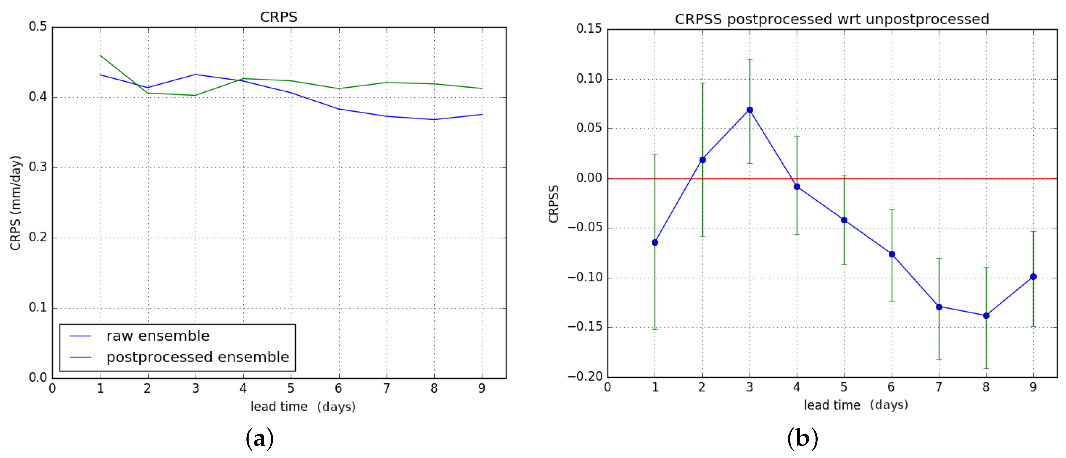
Finally, we look at the CRPS and the improvement attained by postprocessing. We compute the CRPS of the raw and postprocessed forecasts, and subsequently the CRPSS of the postprocessed forecast is computed with the CRPS of the raw forecast as the reference.
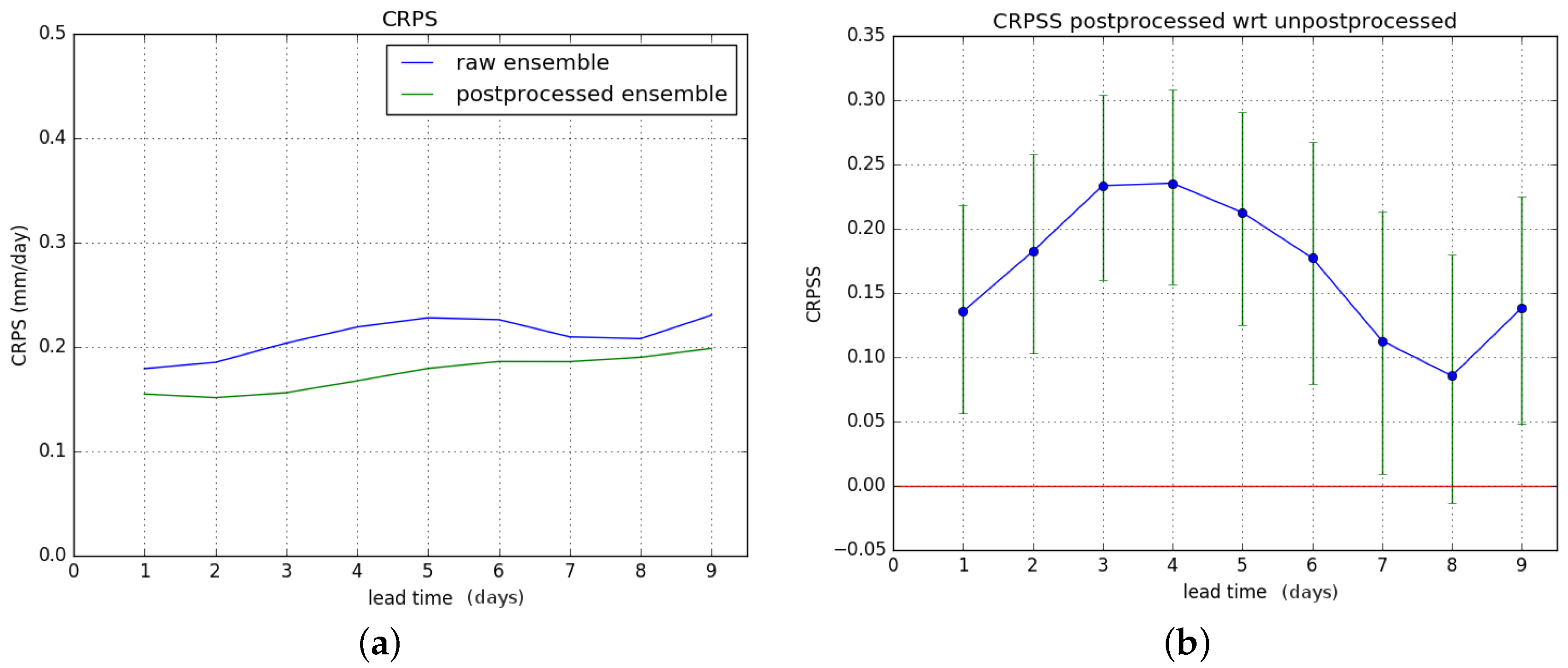
In Figure 10, we consider the entire verification period. Figure 10a shows the CRPS for the raw and postprocessed forecasts. Note that unlike the previous figures, Figure 10a doesn’t show skill scores but the CRPS with units of discharge, and which is a negatively oriented measure (lower is better). Figure 10b shows the CRPSS of the postprocessed forecasts with respect to the raw ones. The results for hydrological winter and hydrological summer are shown in Figure 11 and Figure 12 respectively.
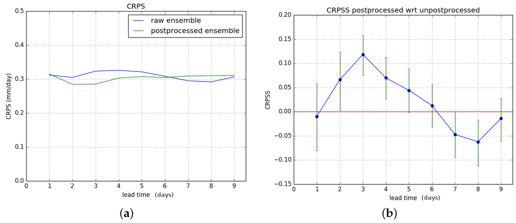
Figure 10.
CRPS and CRPSS improvement for entire verification period. (a) CRPS comparison; (b) Improvement due to postprocessing.
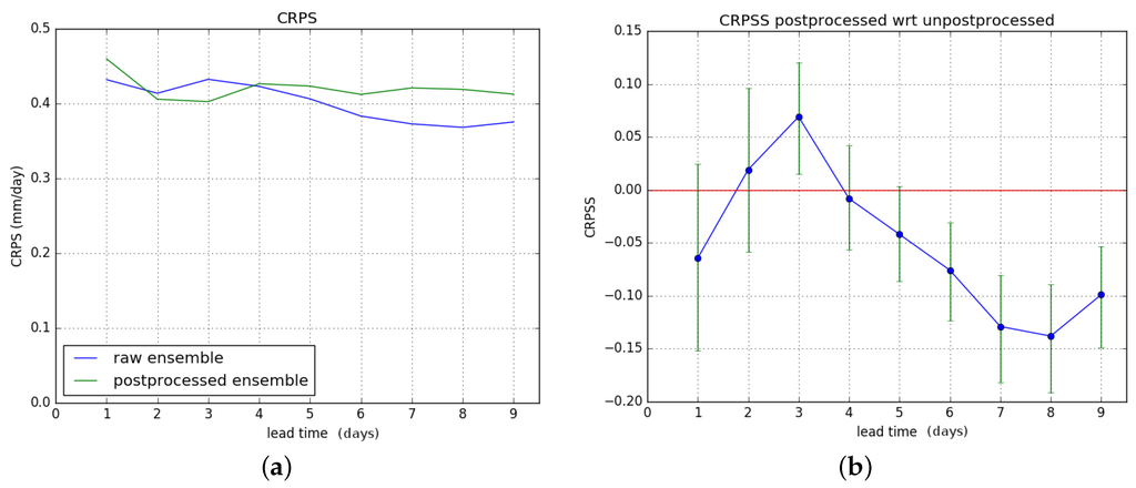
Figure 11.
Continuous Ranked Probability Score (CRPS) and Continuous Ranked Probability Skill Score (CRPSS) improvement for hydrological winter. (a) CRPS comparison; (b) Improvement due to postprocessing.
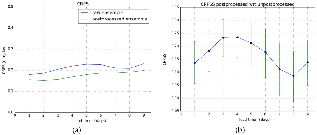
Figure 12.
CRPS and CRPSS improvement for hydrological summer. (a) CRPS comparison; (b) Improvement due to postprocessing.
Results show an overall significant improvement of the CRPS during hydrological summer. For hydrological winter, no significant improvement is gained, and there is degrading of skill for lead times of six days or more. These results combine to give a significant overall improvement in CRPSS for lead times of two to four days for the entire verification period. The overall improvement is less than for the Brier Score.
We also looked at the CRPS for the “perfect hydrological model” setup. Results show only a significant improvement in CRPSS for the summer period, two to four days ahead.
We see that the postprocessing method helps remove some error in the precipitation forecasts during summer. In [7], the authors considered the separate postprocessing of precipitation forecasts before using these as input to a hydrological model, and also found a significant improvement during hydrological summer.
We also compared the ensemble mean of the postprocessed ensemble to the one of the raw ensemble forecast. We find that the bias of the ensemble mean and the mean absolute error (MAE) are not significantly affected by the postprocessing method. The root mean square error (RMSE) of the ensemble mean is actually significantly degraded by the postprocessing method for lead times of two to four days.
When we look at the individual forecasts, we see that unrealistically large discharge values show up in some of the postprocessed forecasts. These outliers have a large impact on the RMSE of the ensemble average. Further investigation reveals the origin of many of these outliers. They typically arise in situations when there is an outlier in the precipitation forecasts, giving rise to mostly discharge ensemble members with no increase in discharge and one or a few giving a peak in discharge. This peak is then enhanced by the calibration, which is performed on the logarithm of the discharges. The exponentiation amplifies this effect, giving an unrealistically large discharge.
The existence of such large outliers in the postprocessed discharge forecasts is problematic if the method is to be used in an operational hydrological ensemble prediction system that also provides discharge ensemble forecasts to end users (and not just exceedance probabilities). Other transformations besides the log transform have been applied in the literature. For instance, [17] use the log-sinh transform [18] before “dressing” each member of an ensemble discharge prediction with a normally distributed error and converting back to real-world units. Another widely-used technique is the normal quantile transform (NQT), as used in the context of the Hydrological Uncertainty Processor (HUP, [19]). Some authors have also discussed issues with outliers after back-transformation. For example, [20] have shown the difficulties occurring in the inversion of the empirical NQT, if the normal random deviates lie outside the range of historically-observed range. They solve the problem by combining extreme value analysis and non-parametric regression methods. Finally, the Box–Cox transformation is used by [6] in their truncated variant of Ensemble Model Output Statistics (EMOS). In order to avoid positive probabilities for unrealistically high runoff predictions after back-transformation, the normal distributions are right truncated at two times the maximum of the observations.
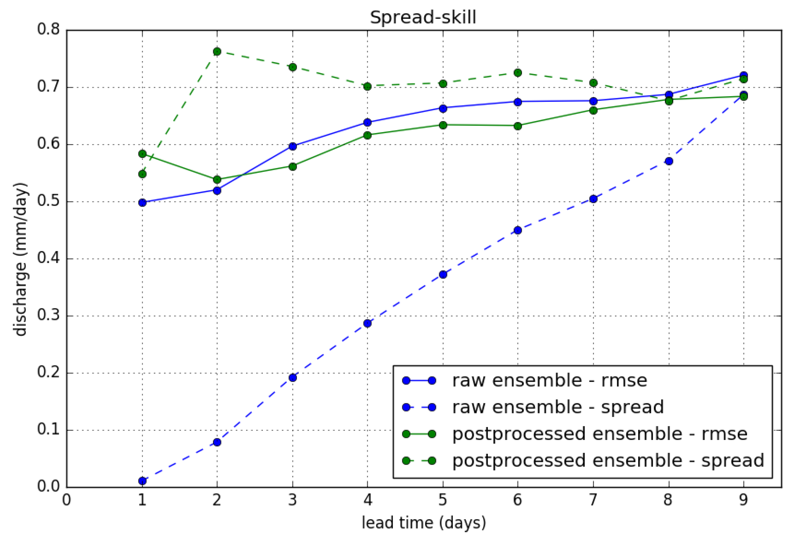
A thorough comparison of different methods to deal with the issue of outliers is outside the scope of this paper. In our study, we tested a truncation of the outliers at two times the maximum of the observations ([6]). Naturally, this leaves the verification results for the exceedance of the P90 threshold (Brier score) unchanged. Moreover, we find that results for the CRPS are not significantly affected. Results for the “spread-skill” relationship after truncation are presented in Figure 13. We show the ensemble spread (or ensemble standard deviation) and RMSE of the ensemble mean, which are equal for a perfectly calibrated ensemble, for the raw and postprocessed ensemble forecasts. We clearly see the effect of the variance inflation method in increasing the spread of the ensemble. The RMSE of the ensemble mean is slightly reduced by the postprocessing, but note that this is dependant on the choice of truncation.

Figure 13.
Ensemble spread and RMSE of the ensemble mean during the entire verification period, after truncation of outliers.
Ideally, a more refined method should be developed to deal with the issue of outliers. We briefly discuss some possible solutions and avenues for further study.
- The reforecast schedule at ECMWF has evolved towards two dates per week, and the reforecast ensembles now consist of 11 members. Having more training data available should increase the chance that a specific forecast with outliers is represented in the past set of reforecasts, and should improve the calibration method. We intend to validate the use of the 11-member reforecasts as soon as enough data is available.
- We are also investigating a postprocessing method with separate calibration for different river discharge regimes (rising or falling limb).
- There is a trade-off between the sample size and the refinement of the calibration. It could be checked that some key characteristics of the hydrological ensemble to be postprocessed (for instance, its spread or its range) are sufficiently well-represented in the hydrological reforecast dataset used for calibration. In case they are not well represented, the postprocessing can be skipped.
6. Conclusions
We investigated the postprocessing of our discharge forecasts for the Ourthe catchment, using archived weekly ECMWF five-member reforecasts that have been available since 2012. We used these as input to create a set of hydrological reforecasts. The implemented calibration method is the variance inflation method as adapted by [7].
Verification results indicate that the postprocessing method gives a significant improvement in the Brier skill score for lead times of up to five days. This can be attributed to:
- An improvement over the entire forecast range during hydrological summer, mainly reducing false alarms.
- An improvement during winter for the first three days, and a degrading of the forecast skill for the last three days.
For the CRPS score, which measures the overall probabilistic skill, the improvement is less than for the Brier score, but still significant for the entire forecast range during hydrological summer. For hydrological winter, there is not much improvement, and a degrading of the skill for lead times of six days or more. We conclude that it is definitely valuable to apply the postprocessing method during hydrological summer. In our operational setting, where discharge exceedance probabilities for higher thresholds are forecast, the method is also useful during winter, but not for lead times beyond five days.
Finally, the postprocessed discharge forecasts contain some unrealistically large outliers. The RMSE of the ensemble mean is actually degraded by the method. This is caused by outliers in the raw ensemble discharge forecasts that are further amplified by the non-linear back-transformation to the corrected discharge values.
This leads us to conclude that the variance inflation method is suitable when the aim is to improve the forecasting of discharge exceedance probabilities. The method delivers forecasts with improved statistical properties. However, it fails to always deliver realistic ensemble forecasts when the individual members are considered. Thus, if the aim is to deliver actual postprocessed ensemble discharge forecasts (or a visualization with, for example, spaghetti plots, …) to an end user, other methods should be considered or the variance inflation method needs at least further refinement. We intend to discuss this issue further in a following study.
Acknowledgments
We would like to thank Bert Van Schaeybroeck and Stephane Vannitsem for useful discussions. We thank Philippe Dierickx and Marina Thunus of the Service Public de Wallonie (SPW) for providing discharge data for the Ourthe. Finally, we thank the three anonymous referees for their helpful comments and suggestions.
Author Contributions
Both authors contributed equally to the development of the methodology, the data analysis, drawing the conclusions, and the writing of the manuscript.
Conflicts of Interest
The authors declare no conflict of interest.
References
- Cloke, H.; Pappenberger, F. Ensemble flood forecasting: A review. J. Hydrol. 2009, 375, 613–626. [Google Scholar] [CrossRef]
- Roulin, E.; Vannitsem, S. Skill of medium-range hydrological predictions. J. Hydrometeorol. 2005, 6, 729–744. [Google Scholar] [CrossRef]
- Jaun, S.; Ahrens, B. Evaluation of a probabilistic hydrometeorological forecast system. Hydrol. Earth Syst. Sci. 2009, 13, 1031–1043. [Google Scholar] [CrossRef]
- Fundel, F.; Zappa, M. Hydrological ensemble forecasting in mesoscale catchments: Sensitivity to initial conditions and value of reforecasts. Water Resour. Res. 2011. [Google Scholar] [CrossRef]
- Thielen, J.; Bartholmes, J.; Ramos, M.H.; de Roo, A. The European Flood Alert System—Part 1: Concept and development. Hydrol. Earth Syst. Sci. 2009, 13, 125–140. [Google Scholar] [CrossRef]
- Hemri, S.; Lisniak, D.; Klein, B. Multivariate postprocessing techniques for probabilistic hydrological forecasting. Water Resour. Res. 2015, 51, 7436–7451. [Google Scholar] [CrossRef]
- Roulin, E.; Vannitsem, S. Post-processing of medium-range probabilistic hydrological forecasting: Impact of forcing, initial conditions and model errors. Hydrol. Process. 2015, 29, 1434–1449. [Google Scholar] [CrossRef]
- Zalachori, I.; Ramos, M.H.; Garçon, R.; Mathevet, T.; Gailhard, J. Statistical processing of forecasts for hydrological ensemble prediction: A comparative study of different bias correction strategies. Adv. Sci. Res. 2012, 8, 135–141. [Google Scholar] [CrossRef]
- Verkade, J.; Brown, J.; Reggiani, P.; Weerts, A. Post-processing ECMWF precipitation and temperature ensemble reforecasts for operational hydrologic forecasting at various spatial scales. J. Hydrol. 2013, 501, 73–91. [Google Scholar] [CrossRef]
- Van Andel, S.J.; Weerts, A.; Schaake, J.; Bogner, K. Post-processing hydrological ensemble predictions intercomparison experiment. Hydrol. Process. 2013, 27, 158–161. [Google Scholar] [CrossRef]
- Roulin, E.; Vannitsem, S. Postprocessing of Ensemble Precipitation Predictions with Extended Logistic Regression Based on Hindcasts. Mon. Weather Rev. 2012, 140, 874–888. [Google Scholar] [CrossRef]
- Johnson, C.; Bowler, N. On the reliability and calibration of ensemble forecasts. Mon. Weather Rev. 2009, 137, 1717–1720. [Google Scholar] [CrossRef]
- Wood, A.W.; Schaake, J.C. Correcting errors in streamflow forecast ensemble mean and spread. J. Hydrometeorol. 2008, 9, 132–148. [Google Scholar] [CrossRef]
- Bultot, F.; Dupriez, G. Conceptual hydrological model for an average-sized catchment area, II. Estimate of parameters, validity of model, applications. J. Hydrol. 1976, 29, 273–292. [Google Scholar] [CrossRef]
- Van den Bergh, J.; Roulin, E. Hydrological ensemble prediction and verification for the Meuse and Scheldt basins. Atmos. Sci. Lett. 2010, 11, 64–71. [Google Scholar] [CrossRef]
- Hersbach, H. Decomposition of the Continuous Ranked Probability Score for Ensemble Prediction Systems. Weather Forecast. 2000, 15, 559–570. [Google Scholar] [CrossRef]
- Pagano, T.C.; Shrestha, D.L.; Wang, Q.J.; Robertson, D.; Hapuarachchi, P. Ensemble dressing for hydrological applications. Hydrol. Process. 2012, 27, 106–116. [Google Scholar] [CrossRef]
- Wang, Q.J.; Shrestha, D.L.; Robertson, D.E.; Pokhrel, P. A log-sinh transformation for data normalization and variance stabilization. Water Resour. Res. 2012. [Google Scholar] [CrossRef]
- Krzysztofowicz, R.; Kelly, K.S. Hydrologic uncertainty processor for probabilistic river stage forecasting. Water Resour. Res. 2000, 36, 3265–3277. [Google Scholar] [CrossRef]
- Bogner, K.; Pappenberger, F.; Cloke, H.L. Technical Note: The normal quantile transformation and its application in a flood forecasting system. Hydrol. Earth Syst. Sci. 2012, 16, 1085–1094. [Google Scholar] [CrossRef]
© 2016 by the authors; licensee MDPI, Basel, Switzerland. This article is an open access article distributed under the terms and conditions of the Creative Commons Attribution (CC-BY) license (http://creativecommons.org/licenses/by/4.0/).


