Evaluating Rainfall Forecast Skill in Numerical Weather Prediction Models and the Effects of Bias Correction on the PCJ (Piracicaba-Capivari-Jundiaí) River Basins in Brazil

Abstract

Precipitation forecasts from numerical weather prediction systems can contain systematic errors in both occurrence and magnitude, limiting their usefulness for hydrological applications. This study evaluated two operational precipitation forecasting systems against two observational reference datasets across three basins in São Paulo State, Brazil, and assessed statistical post-processing for dry/wet occurrence and precipitation magnitude. Four logistic-regression-based methods were evaluated for occurrence correction, while Quantile Delta Mapping (QDM) was applied to precipitation amounts. Occurrence correction was assessed using POD, FAR, CSI, and ACC, with dry days defined as the event. Changes in individual classifications were evaluated using the exact McNemar test, while changes in categorical metrics across seven lead times were assessed using exact paired permutation tests and bootstrap 95% confidence intervals. A descriptive multi-metric ranking was used to compare correction methods. QDM was evaluated using RMSE skill score and KGE. Occurrence correction modified categorical performance, with effects depending on forecast–observation pairing, basin, and lead time. The McNemar test identified significant classification changes after Holm adjustment in some configurations, whereas the permutation tests did not provide evidence of systematic metric improvement. HBLR-AR1 showed the most balanced overall performance, whereas LR-Seasonal was the least consistent method. QDM improved RMSE skill, particularly at longer lead times, but did not consistently improve KGE. Overall, correction effectiveness depended on forecast–observation discrepancies.

1. Introduction

Hydrometeorological forecasting integrates meteorological predictions with hydrological modeling to estimate catchment dynamics, supporting critical applications from real-time flood early warning systems to long-term water resource management (Sene, 2010) [1]. However, the reliability of streamflow simulations remains highly constrained by the quality of atmospheric forcing inputs—particularly precipitation data—which frequently suffer from systematic biases and misrepresentations within numerical weather prediction (NWP) systems [2]. Both process-based and data-driven hydrological models propagate these input errors nonlinearly through their systems. While process-based frameworks rely on simplified structural representations of complex land-surface interactions, data-driven approaches—including recent machine learning architectures—frequently exhibit high sensitivity to the representativeness of historical training datasets and lack operational interpretability [3,4]. Consequently, mitigating systematic errors in raw NWP outputs remains a critical challenge for improving operational hydrological forecasting. Previous studies have shown that the choice of bias-adjustment strategy can substantially influence the resulting precipitation and hydrological simulations [5,6].

To address these systematic discrepancies, statistical post-processing techniques are widely employed to align forecast distributions with observations. Distribution-based methods such as Quantile Mapping (QM) have demonstrated considerable success in correcting precipitation biases, particularly in terms of mean and variance characteristics [7]. However, their effectiveness is not universal, as they may exhibit limitations in correcting timing errors and, in some cases, may even degrade forecast performance under highly variable or convective precipitation regimes [8]. Furthermore, their performance is often sensitive to temporal resolution, with forecast skill generally decreasing as the time scale becomes finer [9].

The literature reports a wide range of approaches for correcting systematic errors in NWP forecasts, including Quantile Mapping, Bayesian Model Averaging, and regression-based techniques, all of which aim to improve forecast quality [10,11,12]. Among these methods, Quantile Delta Mapping (QDM), which explicitly preserves relative changes in quantiles, has been widely applied to bias correction of global climate model (GCM) outputs [13,14,15]. However, to the best of our knowledge, the application of QDM to operational numerical weather prediction (NWP) forecasts remains limited. The available literature includes its application to the ERA5-Land reanalysis dataset [9] and to long-term, coarse-resolution climate model simulations, such as those from the BNU-ESM model [16]. More recently, Jiao et al. [17] compared traditional QDM with their proposed observation-based quantile delta mapping (OB-QDM) approach for correcting general circulation model (GCM) outputs. In contrast, the most recent study that specifically investigated bias-correction methods to improve precipitation forecast skill from NWP models over the Ouémé River basin in Benin was conducted by Bossa and Hounkpé [18]. That study compared three methods—empirical quantile mapping, parametric quantile mapping, and linear scaling—but did not explicitly investigate QDM for correcting NWP precipitation forecasts. On the other hand, Golian and Murphy [19] explicitly used QDM, but for correcting monthly ECMWFs (SEAS5). Therefore, a gap remains regarding the application and evaluation of QDM for systematic bias correction of NWP precipitation forecasts at daily resolution, which this study aims to address.

In catchments characterized by rapid hydrological responses and highly intermittent precipitation, accurately identifying transitions between dry and wet conditions can be as important as estimating rainfall magnitude. Accordingly, precipitation occurrence has been explicitly modeled in statistical post-processing and forecasting frameworks, including logistic-regression-based approaches that calibrate the probability of precipitation occurrence from numerical weather prediction (NWP) ensembles [20,21,22,23,24]. Bayesian approaches have also been applied to probabilistic precipitation forecasting and post-processing. For example, Bayesian Model Averaging (BMA) has been used for ensemble precipitation forecasts to account for both the probability of zero precipitation and the distribution of positive precipitation amounts [23,25]. More recently, Yadav and Yadav [26] conducted a comparative evaluation of six statistical post-processing methods—censored Non-homogeneous Logistic Regression (cNLR), BMA, logistic regression (LogReg), heteroscedastic logistic regression (hLogReg), heteroscedastic extended logistic regression (HXLR), and ordered logistic regression (OLR)—for short-range precipitation forecasts from the NCMRWF Ensemble Prediction System (EPS) over the Vishwamitri River Basin. Their results showed that cNLR provided the best overall calibration performance across the five grid points based on the Brier Score (BS) and area under the curve (AUC), whereas BMA and hLogReg showed comparatively poorer performance. In addition, hierarchical Bayesian models have been developed to jointly represent precipitation occurrence and amounts [27]. Beyond NWP forecast post-processing, Markov-chain-based approaches have also been developed for precipitation bias correction and have been successfully applied to reproduce precipitation occurrence sequences and wet- and dry-spell characteristics in global climate model (GCM) data [28]. Collectively, these studies demonstrate the potential of both frequentist and Bayesian frameworks, as well as stochastic occurrence-based approaches, for improving the representation of precipitation occurrence and amounts in precipitation prediction and bias correction.

In South America, and particularly in Brazil, Bayesian approaches have also been applied to precipitation-related forecasting problems. Coelho et al. [29] developed a Bayesian forecast-assimilation framework to produce calibrated and downscaled seasonal rainfall forecasts, while Lima and Lall [30] employed a hierarchical Bayesian framework to identify the onset and cessation of the rainy season in northeastern Brazil using daily rainfall occurrence data. More recently, Pinheiro and Ouarda [31] proposed a Bayesian adaptation of the TelNet neural-network model for seasonal precipitation forecasting and calibration across South America using ERA5 reanalysis data and historical simulations from 18 CMIP6 climate models. However, these studies have primarily focused on seasonal forecasting, rainfall-season characterization, reanalysis, or climate-model simulations rather than the correction of precipitation occurrence in short- to medium-range NWP forecasts. Thus, although both frequentist regression and Bayesian approaches have been explored for precipitation prediction and post-processing, the use of hierarchical Bayesian logistic regression with Markov chain Monte Carlo (MCMC) specifically to correct dry/wet occurrence in short- to medium-range NWP precipitation forecasts, together with a direct comparison with its corresponding frequentist formulation, remains limited.

The hydrological and forecasting challenges described above are particularly relevant in the Piracicaba, Capivari, and Jundiaí (PCJ) River Basin in southeastern Brazil. Characterized by dynamic land-use transitions, where extensive sugarcane cultivation interfaces with rapid urban and industrial expansion, the PCJ Basin serves as the headwater source for the Cantareira System, a vital inter-basin water-transfer network supplying more than 14 million people [32]. In this region, localized convective systems and frontal interactions contribute to substantial uncertainty in NWP precipitation forecasts [33]. Errors in precipitation occurrence during seasonal dry-to-wet transitions can have important operational consequences, potentially affecting flood-control decisions and reservoir replenishment. Improving categorical forecast skill by reducing false alarms and missed events is therefore particularly relevant for regional water-resource management.

This study addresses these operational and methodological gaps by investigating two complementary aspects of precipitation forecast post-processing. First, it evaluates the effectiveness of Quantile Delta Mapping (QDM), a method predominantly used for climate-model bias correction, in improving short-term daily precipitation forecasts. Second, it examines whether frequentist and hierarchical Bayesian logistic regression frameworks can improve the correction of dry/wet precipitation occurrence. The approaches are evaluated across three basins within the PCJ system, using two forecast datasets, two observational references, and multiple forecast lead times. This framework provides a comprehensive assessment of the applicability and generalizability of these post-processing approaches in regions characterized by high precipitation variability and rapid hydrological responses.

Specifically, the objectives of this study are threefold: (i) to evaluate the raw verification performance of precipitation forecasts from the SIMEPAR operational forecasting system and the ECMWF ensemble framework across the hydrologically and meteorologically complex PCJ Basin; (ii) to assess the effectiveness of Quantile Delta Mapping (QDM) in mitigating intensity-related forecast biases across increasing forecast lead times; and (iii) to investigate whether explicit occurrence-based corrections using frequentist logistic regression and hierarchical Bayesian logistic regression systematically improve categorical precipitation-event identification across forecast lead times and forecast–observation configurations.

The results indicate that the effectiveness of statistical post-processing depends strongly on the characteristics of the underlying forecast errors and the verification metric considered. While occurrence-based correction methods generally improved precipitation-event detection, these gains were accompanied by trade-offs between hit rates and false alarms. Overall, the findings highlight both the potential and the limitations of increasingly complex statistical correction frameworks for improving precipitation forecasts used in operational hydrological applications.

2. Materials and Methods

2.1. Study Area and Data

The PCJ River Basins (Piracicaba, Capivari, and Jundiaí) cover approximately 15,300 km² across the states of São Paulo and Minas Gerais, Brazil, encompassing 76 municipalities. The region plays a strategic role in urban, industrial, and agricultural water supply, including contributions to the Campinas and São Paulo Metropolitan Regions via the Cantareira Water Supply System.

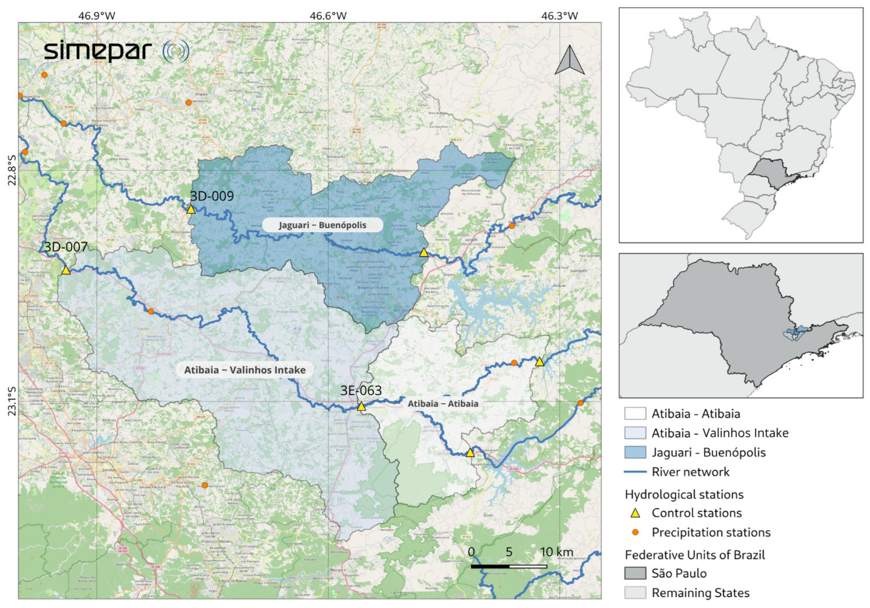
Operational hydrometeorological forecasting is conducted through the PCJ Hydrometeorological Forecasting System (SPHM-PCJ), which provides meteorological forecasts for municipalities and streamflow forecasts at three control stations: Atibaia River at Atibaia (62669900, 3E-063T) (Atibaia-Atibaia), Atibaia River at Valinhos intake (62678150, 3D-007T) (Atibaia- Valinhos Intake), and Jaguari River at Buenópolis (62605000, 3D-009T) (Jaguari-Buenópolis).

The forecasting system was developed by SIMEPAR to provide operational hydrometeorological forecasts that support River Basin Committees in real-time reservoir operation and strategic water supply management. It also enables the estimation of the probability that forecasted streamflow will fall below the minimum thresholds established by Joint Resolutions ANA/DAEE No. 925 and 926/2017 [34]. The hydrometric control stations are located downstream of the Cantareira reservoir system [35]. For modeling purposes, three incremental sub-basins contributing to these control points were delineated based on topographic drainage divides (Figure 1).

Four datasets were analyzed: two observational references and two forecast products. The observational and forecast datasets have different periods of record. However, to ensure a consistent evaluation, all analyses presented in this study were performed using only the common overlapping period from 7 September 2019 to 20 March 2024. The temporal coverage reported below refers to the full availability of each dataset. For the purposes of this study, all datasets were referenced to the same local time (UTC-3) and processed to a common daily temporal resolution, ensuring temporal consistency throughout the analyses.

The first observational dataset consists of rain gauge stations operated by SPHM-PCJ, with records available from 10 August 2018 (OBS-STN; hereafter). The stations provide precipitation observations at sub-daily temporal resolutions. For this study, the observations were aggregated to daily precipitation totals after applying basic quality-control procedures, including the removal of negative values and physically unrealistic precipitation amounts. The quality-controlled daily precipitation was then averaged within each basin to obtain basin-mean precipitation. However, gauge density is limited, with one basin containing up to four stations and the remaining basins containing only two stations.

To complement these point-based measurements and account for the spatial heterogeneity of precipitation—particularly during localized convective events—the Brazilian Daily Weather Gridded Data (BR-DWGD; hereafter OBS-GRD) was integrated into the analysis. This product provides daily gridded meteorological variables at 0.1° × 0.1° spatial resolution from 1 January 1961 to 20 March 2024 [36]. Basin-averaged precipitation was obtained by extracting the grid cells intersecting each basin and calculating the arithmetic mean of the corresponding precipitation values.

While OBS-GRD enhances the representation of spatial patterns, its utility is restricted to the historical period ending in March 2024. Consequently, OBS-STN serves as the critical reference for assessing operational consistency and real-time forecast applicability through 2026. This dual-reference approach ensures that the performance of the forecasting systems is evaluated against both the high-precision local gauge data and the broader spatial context provided by the gridded product.

The forecast datasets used in this study consist of two products. The first is the operational forecast produced by the SIMEPAR (hereafter FCST-SIM), an operational high-resolution regional forecast developed by SIMEPAR. This system utilizes the Weather Research and Forecasting (WRF) model configured with a 5 km horizontal grid version 4.1.2 [37], providing daily accumulated precipitation for lead times up to seven days. The study period for this dataset spans January 2019 to the present.

SIMEPAR (Technology and Environmental Monitoring System of Paraná) is a non-profit organization dedicated to promoting sustainable socio-economic development through weather forecasting and the operation of an integrated hydrometeorological monitoring network. In addition, SIMEPAR develops hydrological modeling and geointelligence solutions to support decision-making in sectors such as energy, sanitation, and civil defense. SIMEPAR products are available upon request and can also be accessed through SIMEPAR’s official website https://www.simepar.br/ (accessed on 6 September 2026).

The second dataset comprises forecasts from the European Centre for Medium-Range Weather Forecasts Integrated Forecasting System (IFS), specifically its ensemble prediction system (FCST-ENS), consisting of 51 ensemble members. The forecasts correspond to operational ECMWF products and were retrieved in real time as released. The data were obtained on regular grids with spatial resolutions of 0.4°, 0.2°, and 0.1° (approximately 44 km, 22 km, and 11 km), spanning September 2019 to the present.

All datasets (OBS-STN, OBS-GRD, FCST-SIM, and FCST-ENS) were spatially averaged over each basin. After removing missing values, a total of 1648 daily observations were retained for analysis. Of these, 1318 daily observations comprised the training dataset, covering the period from 7 September 2019 to 21 April 2023, while the remaining 330 observations comprised the testing dataset, covering the period from 22 April 2023 to 20 March 2024.

2.2. Bias Correction Procedure

Bias correction of precipitation amounts was performed using QDM for both the FCST-SIM and Ensemble Prediction System (ENS) forecasts across the seven lead times, using both observational references for calibration. The FCST-ENS consists of 51 individual ensemble members; therefore, QDM was applied independently to each member. Following correction, the median of the 51 corrected ensemble members was used as the deterministic predictor for the test dataset, as it provides a robust estimate of the ensemble central tendency while reducing the influence of individual members with anomalous values. The rationale for selecting the ensemble median as the deterministic predictor is presented in Section 2.2.1. The resulting forecasts were then evaluated against the two observational references.

Ideally, bias correction procedures should be calibrated and evaluated using independent training, validation, and testing subsets (e.g., 60–20–20%). However, due to the relatively limited sample size, the dataset was divided into two subsets: 80% for training and 20% for testing. The correction parameters were estimated using the training data and evaluated on the testing subset to ensure independent performance assessment while maintaining sufficient data for robust parameter estimation.

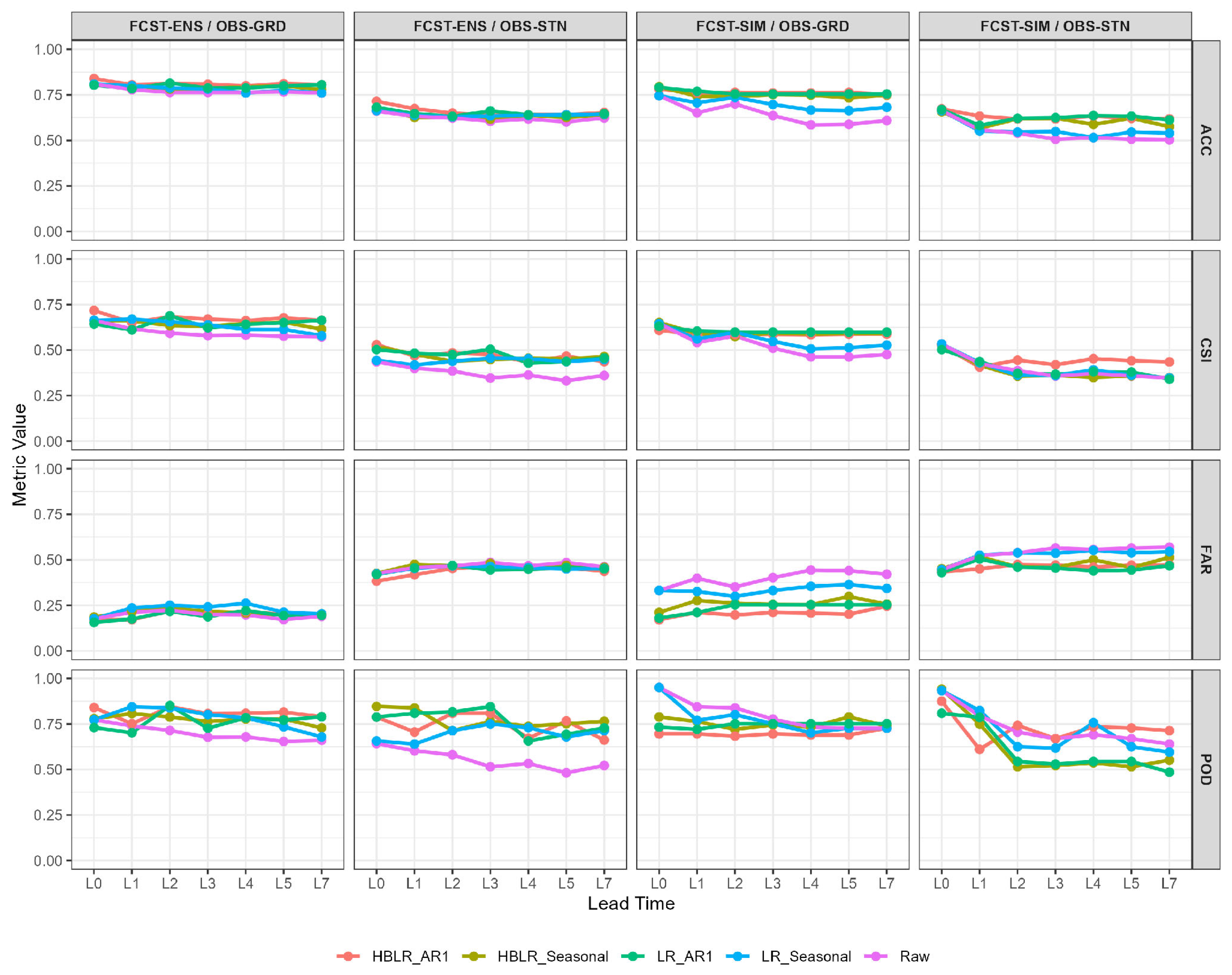
For the wet/dry occurrence analysis, a range of correction models with increasing levels of complexity were evaluated within both frequentist and Bayesian frameworks. For the ENS forecasts, the ensemble median was used as the deterministic predictor representing the 51 individual ensemble members in the occurrence-correction analysis. The occurrence-correction models were evaluated on the test dataset for all three basins, four forecast–observation pairings (FCST-SIM/OBS-STN, FCST-SIM/OBS-GRD, FCST-ENS/OBS-STN, and FCST-ENS/OBS-GRD), and seven forecast lead times. Performance was assessed using the categorical verification metrics described in Section 3.2, allowing comparison of the consistency and effectiveness of the correction approaches across basins, forecast–observation pairings, and lead times. All the occurrence-correction model parameters, classification thresholds, and monthly wet-day probabilities were derived strictly from the training data to avoid data leakage.

2.2.1. Selecting the Ensemble Predictor

In some cases, it is more appropriate to use a representative ensemble statistic rather than all ensemble members individually, as ensemble summary predictors provide a more compact representation of the forecast distribution [24].

Before selecting a deterministic predictor from the ECMWF ensemble, four ensemble summary statistics (mean, median, 25th percentile, and 75th percentile) were evaluated across the three basins, two observational references, and seven forecast lead times using Bias, RMSE, and the Kolmogorov–Smirnov (KS) statistic. For each metric, the four predictors were ranked from the smallest to the largest value, assigning rank 1 to the best-performing predictor and rank 4 to the worst-performing predictor. The Total Rank for each predictor was then calculated as the sum of its ranks across the three evaluation metrics. To obtain a generalized assessment of predictor performance, the Total Rank values were averaged across the three basins, two observational references, and seven forecast lead times. The ensemble predictors were subsequently ordered according to the average Total Rank, with lower values indicating better overall performance.

As shown in

Table 1. Average ranking of deterministic ensemble summaries across all basins, observational references, and lead times, ordered by increasing Overall Rank.

Predictor	Bias Rank	RMSE Rank	KS Rank	Overall Rank
Median	1.07	1.64	1.86	4.57
Q25	2.52	1.50	1.14	5.17
Mean	2.40	2.86	4.00	9.26
Q75	4.00	4.00	3.00	11.00

, the ensemble median achieved the lowest average overall rank (4.57), indicating the best overall performance among the evaluated predictors. Although the 25th percentile showed slightly better performance in terms of RMSE and KS, the ensemble median exhibited substantially lower bias, resulting in the best overall ranking. Therefore, the ensemble median was selected as the deterministic predictor for the subsequent occurrence-correction analyses and for evaluating forecast performance after magnitude correction.

2.2.2. Quantile Delta Mapping QDM

The correction was implemented using the Quantile Delta Mapping (QDM) method, a distribution-based extension of classical Quantile Mapping (QM). In standard QM, simulated values are adjusted by aligning their cumulative distribution function (CDF) with that of the observations over a reference period, thereby correcting systematic biases in the modeled distribution.

Quantile Delta Mapping (QDM) extends the Quantile Mapping (QM) framework by preserving changes in quantiles, rather than correcting absolute values, thereby maintaining the model-simulated change signal while correcting systematic biases relative to observations. In climate applications, this corresponds to preserving projected changes in quantiles while adjusting the modeled distribution to match observed conditions. QDM has been shown to perform well in preserving distributional characteristics and extremes [13,38].

The algorithm of QDM starts by extracting the non-exceedance probability of the model value at time t and p_FCST,test from the empirical CDF of the projected (here, the test) series x_FCST,test:

$$p_{FCST,test} \left(t\right) = F_{FCST,test}^{\left(t\right)}\left[x_{FCST,test}\left(t\right)\right], p_{FCST,test}\left(t\right) \in \left\{\mathrm{0,1}\right\}$$

(1)

The relative change in quantiles between the projected (test) and historical (train) is given by the following:

$${∆}_{FCST}\left(t\right) = {\displaystyle \frac{F_{FCST,test}^{\left(t\right)-1}\left[p_{FCST,test}\left(t\right)\right]}{F_{FCST,train}^{-1}\left[p_{FCST,test}\left(t\right)\right]}}= {\displaystyle \frac{x_{FCST,test}\left(t\right)}{F_{FCST,train}^{-1}\left[p_{FCST,test}\left(t\right)\right]}}$$

(2)

The bias-corrected precipitation x_QDM,test is derived using the inverse CDF estimated from observed values F⁻¹_OBS,train $F_{OBS,train}^{-1}$, which is then scaled by multiplying by the relative change factor:

$$x_{QDM,test}\left(t\right) = F_{OBS,train}^{-1}\left[p_{FCST,test}\left(t\right)\right]{∆}_{FCST}\left(t\right)$$

(3)

QDM was implemented using the QDM() function from the R package MBC, following the quantile delta mapping algorithm of Cannon et al. (2015) [38]. Correction was applied univariately and separately for each lead time; no seasonal stratification was performed. For each lead time, the empirical distributions of observed and raw modeled values were estimated non-parametrically from the training sample using Type-7 plotting positions, with no parametric distribution fitted and no subsampling (all training values used as empirical quantiles). Because precipitation is a ratio quantity, correction was multiplicative (ratio = TRUE); the package default trace threshold of 0.05 mm/day was used, below which values were treated as exact zeros, with the near-zero correction factor separately bounded (ratio.max.trace = 0.5). The multiplicative correction factor for wet-day values was capped at 2× (ratio.max = 2) to prevent unbounded extrapolation for extreme quantiles. Tied values were resolved by rank order of occurrence (ties = ‘first’), with no jittering applied. Calibration used the first 80% of the chronologically ordered dataset per lead time (training period), and correction was applied strictly out-of-sample to the subsequent, non-overlapping 20% (test period).

To preserve full chronology and strictly avoid the use of future information, the operational application of the method transforms the static train and test periods for each lead time into a dynamic rolling window. To illustrate this dynamic approach, consider a 6-day lead time (L6) forecast with a target date of 7 January, which is generated and issued on January 1st. For this specific lead time, we construct a 360-day rolling window of past forecasts ending on the target date (7 January). This window contains the L6 forecast targeting 7 January, the L6 forecast targeting 6 January, 5 January, and so forth, rolling backward. Because this is treated as an independent L6 series, the forecast targeting 7 January was issued on 1 January, and the forecast targeting 6 January was issued on 31 December. Therefore, at the exact moment of issuance (1 January), every single forecast value within that 360-day test window has already been generated. No forecast in this calculation utilizes an issue date after 1 January. Furthermore, the remaining historical period used to construct the baseline CDFs (both historical observations and forecasts) entirely precedes this 360-day window. By anchoring the rolling window to the target date of an independent lead-time series, the latest issue date inside the calculation window is always exactly the current issue date, ensuring the mathematical chronology remains strictly out-of-sample.

2.2.3. Frequentist and Bayesian Approaches for Dry/Wet Occurrence Correction

To address systematic errors in the timing of predicted dry and wet weather patterns, several statistical post-processing approaches have been proposed, among which logistic regression remains one of the most widely implemented. In this context, the model is calibrated using a binary response variable where dry conditions are represented by 0 and wet conditions by 1, based on a predefined precipitation threshold (e.g., precipitation > 0.1 mm being classified as a wet day). Days with precipitation less than or equal to 0.1 mm are classified as dry days. The contingency table was constructed using this threshold, with dry days considered the target event.

After model calibration, the probability of precipitation occurrence is estimated for each day and subsequently converted into categorical dry/wet forecasts through the application of a probability threshold. This methodology is commonly applied within the frequentist statistical framework, where model parameters are treated as fixed but unknown values. However, uncertainty in parameter estimation can also be represented explicitly through a Bayesian framework, in which prior information is combined with observed data to obtain posterior distributions of the model parameters. This approach facilitates uncertainty quantification and enables probabilistic inference while maintaining the same underlying logistic regression structure [24].

Because predictor selection and preprocessing can substantially influence model performance [39], several model configurations with progressively increasing complexity were evaluated. This strategy was adopted to investigate how different predictor combinations and model structures affect dry/wet occurrence prediction.

The analysis spans multiple dimensions: three basins, four forecast–observation configurations, seven lead times, two statistical approaches (frequentist and Bayesian), and four model structures. In addition, the original ensemble forecasts consist of 51 members, introducing a further dimension for predictor selection. Given this scope, an initial simplification was necessary to preserve model interpretability and enable comparison across configurations. Based on a prior evaluation of ensemble summary statistics, reported in Section 2.2.1 (Table 1), the ensemble median was selected as a single representative predictor of the ensemble forecast.

The first level of model complexity incorporated seasonal variability through a monthly wet-day probability predictor. This predictor was estimated exclusively from the training dataset to prevent information leakage from the validation period. It represents the climatological likelihood of rainfall occurrence for each month and was included to improve discrimination between dry and wet events under different seasonal precipitation regimes.

For the frequentist framework, the forecast predictor, either the ensemble median or FCST-SIM, was standardized to improve numerical stability and ensure a consistent predictor scale. A binary dry/wet representation of the forecast (D_i) was also included to provide information on the forecast occurrence state. These modifications resulted in the Logistic Regression Seasonal model (LR-Seasonal).

The Bayesian implementation was performed using Markov Chain Monte Carlo (MCMC) sampling through JAGS within the R environment. For each fit, 5000 iterations were discarded as burn-in, followed by 20,000 sampling iterations per chain, with no thinning, resulting in 60,000 post-burn-in draws per parameter. The corresponding hierarchical Bayesian logistic regression model (HBLR-Seasonal) used the same forecast predictors and binary dry/wet representation as the LR-Seasonal model. The model additionally incorporated month-specific intercepts within a hierarchical structure, allowing the monthly intercepts to vary while sharing information through a common hierarchical prior and thereby providing partial pooling across months.

The HBLR-Seasonal model is defined as follows:

Y_i ~ Bernoulli (p_i)

(4)

logit (p_i) = α_m[i] + β₁ X_i + β₂ D_i

(5)

where X_i is the standardized precipitation forecast, and α_m[i] is the intercept associated with month m corresponding to observation i.

The monthly intercepts were modeled hierarchically according to Equation (3):

$${\mathsf{\alpha }}_m ~ N ({\mu }_m, {\tau }_{\alpha }^{-1})$$

(6)

where ${\tau }_{\alpha }^{-1}$ represents the variance component (the inverse of the precision parameter), and the hyperparameter µm corresponds to the historical log-odds of rainfall occurrence for month m, as explained in Equation (7):

$${\mu }_m = \mathit{log} \left({\displaystyle \frac{{\pi }_m}{1-{\pi }_m}}\right)$$

(7)

Here, π_m represents the historical monthly wet-day probability estimated strictly from the training dataset.

The regression coefficients (β_j) were assigned truncated normal priors restricted to positive values to maintain consistency with the positive effects identified in the preliminary frequentist analyses, as shown in Equation (8):

β_j ~ N (1.5, 2⁻¹), with β_j > 0

(8)

The precision parameter controlling the variability among monthly intercepts was assigned a Gamma prior, confirming Equation (9):

$${\tau }_{\alpha } ~ \mathrm{Gamma} (2, 2)$$

(9)

This hierarchical formulation enables partial pooling across months, allowing information sharing across seasons while preserving month-specific variability in precipitation occurrence [40].

As a final stage of model development, the complexity of both statistical frameworks was further increased by incorporating a first-order autoregressive predictor, AR(1). In the present retrospective analysis, the AR(1) predictor was defined as the actual precipitation observation from the day immediately preceding the target day. Because the study was conducted using a fixed historical time series, these observations were available for evaluating the theoretical contribution of the AR(1) predictor across all lead times.

However, this formulation cannot be directly applied in a strict real-time operational forecasting system for longer lead times, because the observation from the day immediately preceding the target day may not yet be available at the forecast issuance time. Therefore, an operational implementation would require the lagged predictor to be constructed sequentially. For lead times for which the previous day’s observation is physically available at the time of forecast issuance, the actual observation can be used as the AR(1) predictor. For subsequent lead times, the unavailable observation should be replaced by the corrected forecast from the preceding lead time. For example, the predictor for L2 would use the corrected forecast obtained for L1. This sequential approach preserves strict temporal chronology and ensures that only information available at the time of forecast issuance is used.

The inclusion of the AR(1) term accounts for the temporal dependence commonly observed in daily precipitation occurrence, where the weather state of a given day is strongly influenced by the atmospheric conditions of the preceding day. Incorporating this term into both the frequentist (LR-AR1) and hierarchical Bayesian (HBLR-AR1) frameworks aimed at capturing the natural persistence characteristics associated with extended wet and dry spells.

Together, these progressive methodological choices resulted in four distinct model configurations with increasing complexity. Their main structural characteristics are summarized in

Table 2. Characteristics of the frequentist and Bayesian logistic regression models developed for dry/wet occurrence correction.

Model	Description
LR-Seasonal	Logistic regression using scaled forecasted data, binary wet/dry FCST, and monthly wet-day probability
HBLR-Seasonal	Hierarchical Bayesian version of LR-Seasonal with monthly intercepts
LR-AR1	LR-Seasonal including an AR(1) predictor to represent temporal persistence
HBLR-AR1	HBLR-Seasonal including an AR(1) predictor to represent temporal persistence

.

The probability threshold used to classify predicted probabilities into dry and wet events was determined through Receiver Operating Characteristic (ROC) curve optimization [24]. The optimal threshold was estimated independently for each model, allowing the classification criterion to adapt to the probabilistic characteristics of each model configuration.

2.3. Assessment Metrics

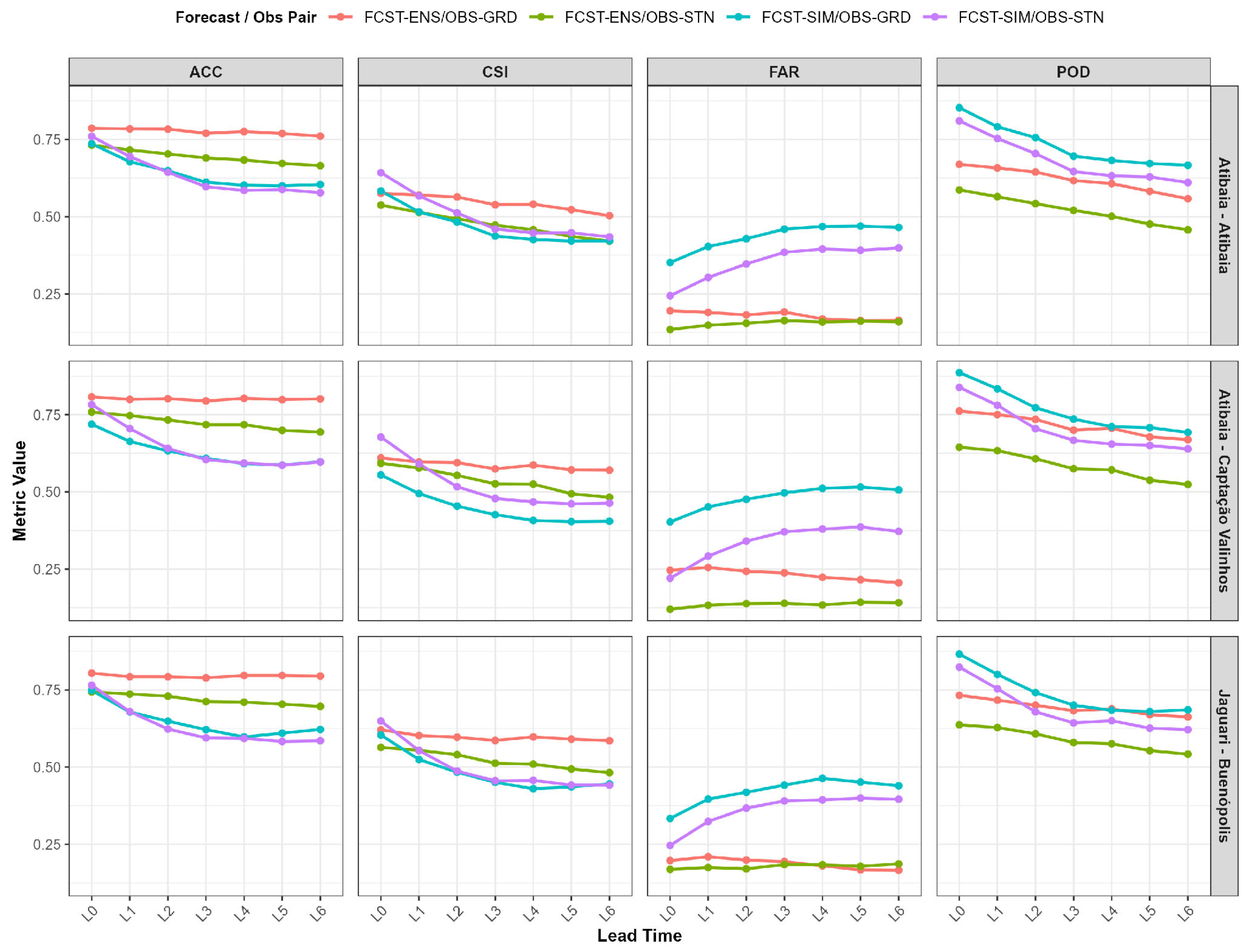
The evaluation of the forecasting models was conducted in two stages. First, the raw forecasts were evaluated using categorical verification metrics to assess their ability to predict the occurrence of dry (zero-rainfall) and wet (non-zero-rainfall) days. In this study, dry days were defined as the target event because of the particular interest in accurately identifying dry conditions in the study area. Accordingly, the contingency table (

Table 3. Contingency table for categorical verification of precipitation occurrence.

FCST/OBS	OBS Dry (0) ≤ 0.1 mm	OBS Wet (1) > 0.1 mm
FCST dry (0) ≤ 0.1 mm	Hits (H)	False alarms (FA)
FCST wet (1) > 0.1 mm	misses (M)	correct negative (CN)

) was defined in terms of hits (H), false alarms (FA), misses (M), and correct negatives (CN), where H represents days correctly classified as dry, FA represents days forecast as dry but observed as wet, M represents days forecast as wet but observed as dry, and CN represents days correctly classified as wet [24].

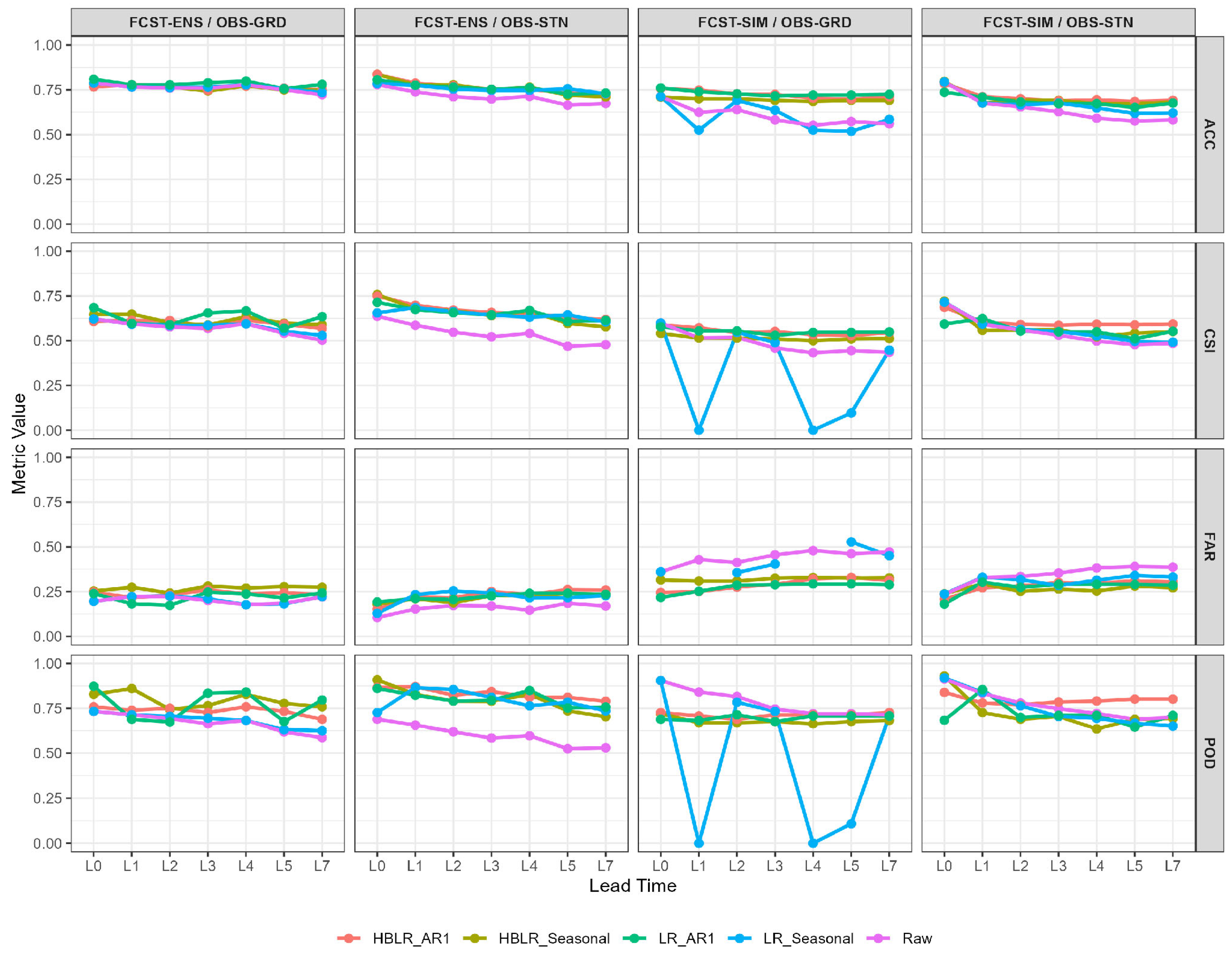
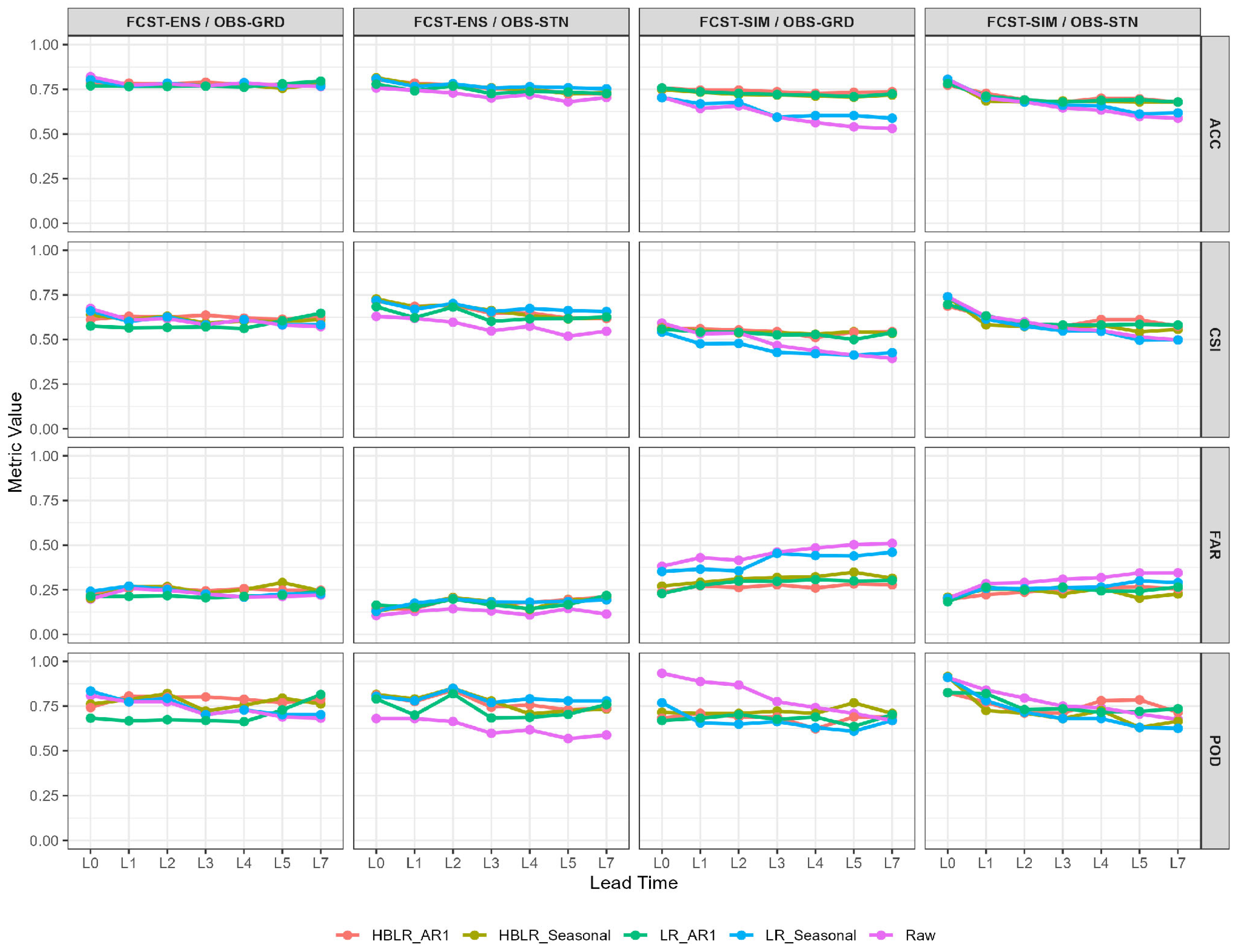
Based on these components, several verification metrics were computed. The Probability of Detection (POD) corresponds to the fraction of observed zero-rainfall days that were correctly forecasted. Accuracy (ACC) represents the fraction of correctly forecasted days, considering both zero-rain and non-zero-rain events. The Critical Success Index (CSI) measures the overall skill of the model in predicting zero-rainfall days. Finally, the False Alarm Ratio (FAR) represents the fraction of predicted zero-rainfall days that did not actually occur [24].

These metrics quantify the ability of the raw models to correctly capture dry and wet weather events. The equations defining each metric are presented in

Table 4. Categorical verification metrics.

Metric	Name	Equation
POD	Probability of Detection	POD = ${\displaystyle \frac{H}{H+M}}$
FAR	False Alarm Ratio	FAR = ${\displaystyle \frac{FA}{H+FA}}$
CSI	Critical Success Index	CSI = ${\displaystyle \frac{H}{H+M+FA}}$
ACC	Accuracy	ACC = ${\displaystyle \frac{H+CN}{H+M+FA+CN}}$

.

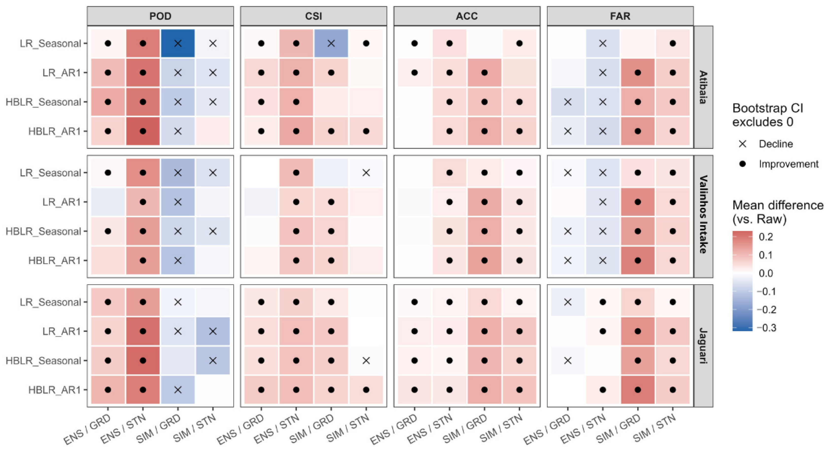
These categorical metrics were used to evaluate the performance of both the raw forecasts and the dry/wet occurrence correction methods. To assess the impact of the occurrence correction on categorical verification metrics, the differences between the corrected and raw forecasts were evaluated. For POD, CSI, and ACC, the difference was calculated as the corrected value minus the raw value. For FAR, the contrast was reversed (raw minus corrected) so that a positive difference consistently represented an improvement in forecast performance across all metrics. Thus, for each basin, forecast–observation pairing, and correction method, seven paired metric differences corresponding to the seven forecast lead times were obtained.

A one-sided exact paired permutation test was applied to the seven paired differences to assess whether the correction produced a systematic improvement across forecast lead times. The null hypothesis was that the paired differences were centered at zero, whereas the alternative hypothesis was that the differences were positive. Bootstrap 95% confidence intervals were also calculated for the paired differences to quantify their uncertainty. Because four correction methods were evaluated for each combination of basin, forecast–observation pairing, and metric, the resulting p-values were adjusted for multiple comparisons using the Holm procedure, with the four correction methods considered as the comparison family within each basin, forecast–observation pairing, and metric.

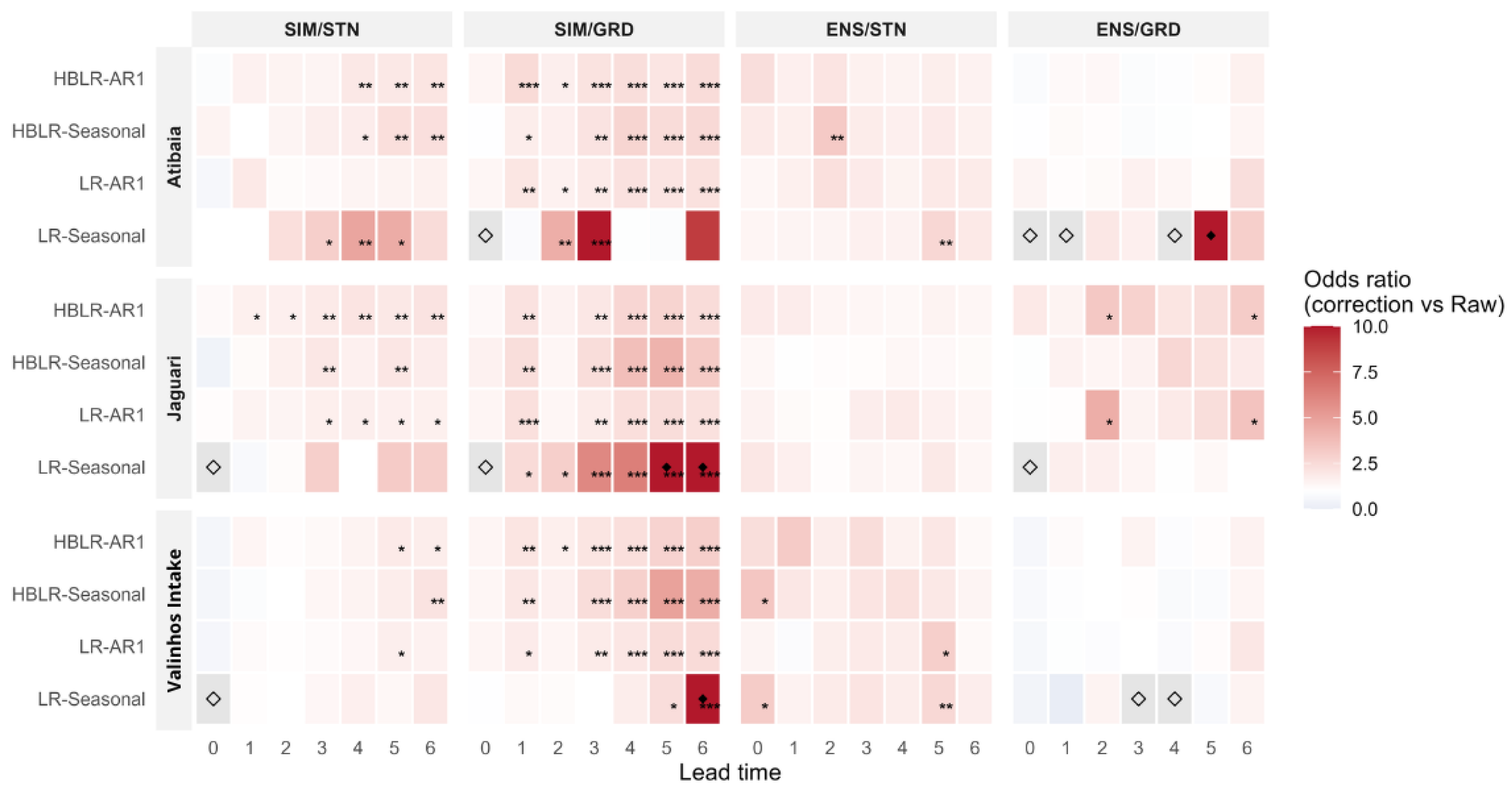
To complement the analysis of changes in aggregated verification metrics, the effect of occurrence correction on the individual paired classification outcomes was assessed using an exact McNemar test. The test was applied separately for each basin, forecast–observation pairing, correction method, and forecast lead time. It evaluates whether the number of cases in which an incorrect raw classification was changed to a correct classification differs from the number of cases in which a correct raw classification became incorrect after correction. The corresponding odds ratio (OR) was calculated as (OR = b/c), where (b) denotes cases incorrectly classified by the raw forecast but correctly classified after correction, and (c) denotes cases correctly classified by the raw forecast but incorrectly classified after correction. Thus, (OR > 1) indicates more corrected errors than newly introduced errors, whereas (OR < 1) indicates the opposite. Exact 95% confidence intervals were calculated for the OR. Because seven lead times were evaluated for each basin, forecast–observation pairing, and correction method, the resulting McNemar p-values were adjusted using the Holm procedure across the seven lead times.

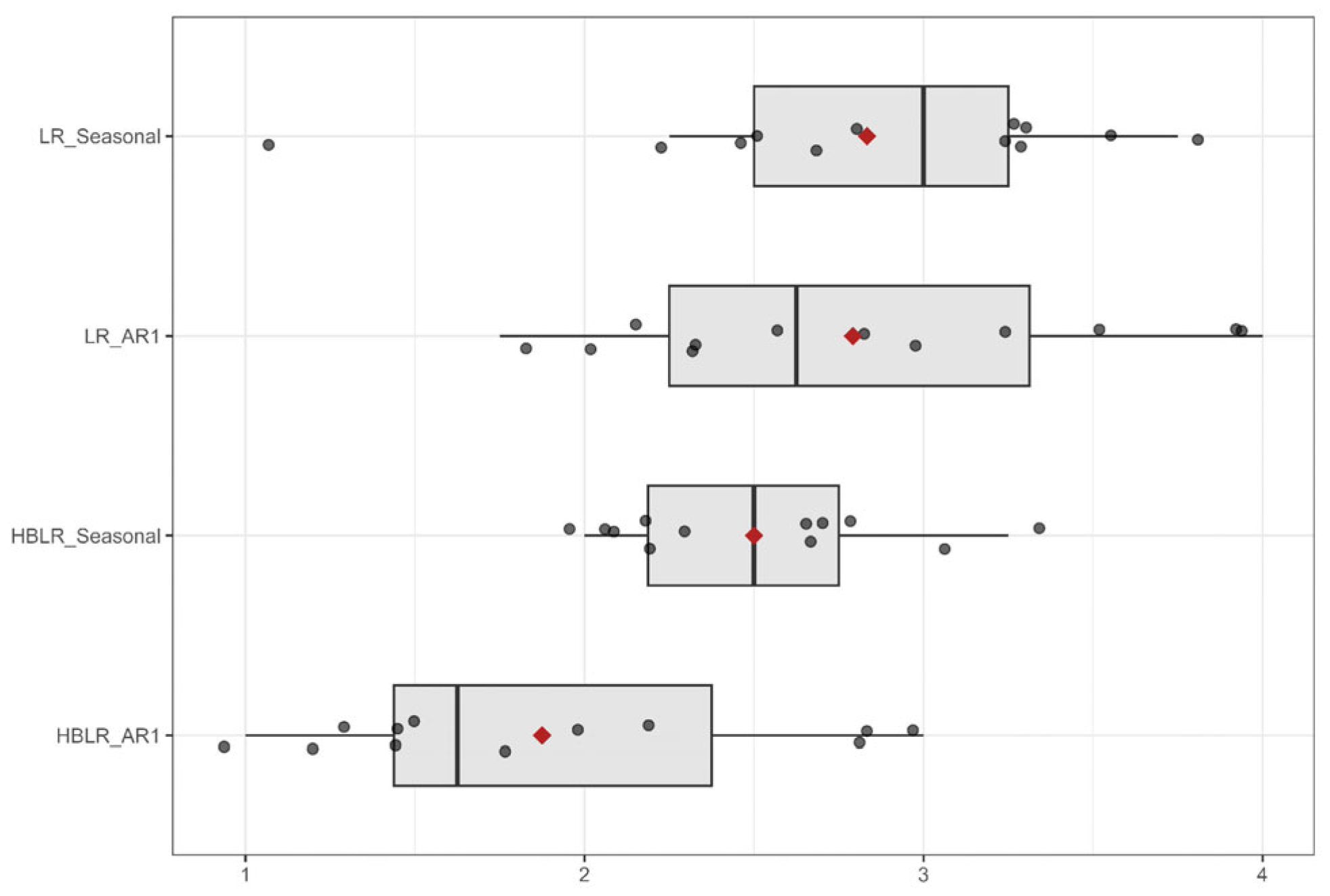
Finally, to provide a more descriptive evaluation of the relative performance of the correction methods and identify the “best” performing method, a descriptive multi-metric ranking procedure was applied. This approach considered the four categorical verification metrics jointly and was used to identify the method providing the most balanced overall performance across POD, CSI, ACC, and FAR.

For this purpose, the values of POD, CSI, ACC, and FAR obtained for each correction method were first averaged across the seven forecast lead times for each basin and forecast–observation pairing. The four correction methods were then compared based on these seven-lead-time averages. For each metric, the four methods were ranked from best to worst, with rank 1 assigned to the best-performing method and rank 4 to the worst-performing method. Higher values were considered better for POD, CSI, and ACC, whereas lower values were considered better for FAR. For example, if the four methods produced mean CSI values of 0.42, 0.45, 0.39, and 0.44, their corresponding ranks would be 3, 1, 4, and 2, respectively. The same ranking procedure was applied independently to POD, ACC, and FAR. An overall rank was then calculated for each correction method as the mean of its four metric-specific ranks.

Because rank 1 represents the best performance for each metric, lower overall ranks indicate better and more balanced performance across the four categorical verification metrics. The correction method with the lowest overall rank was therefore identified as the best-performing method according to the multi-metric evaluation.

Table 5. Summary of the methodological approaches used to assess dry/wet occurrence correction.

Assessment	Purpose	Unit of Analysis	Statistical/Descriptive Approach	Interpretation
Paired classification analysis	Assess whether occurrence correction changes individual dry/wet classifications relative to the raw forecast	Daily classifications, separately for each lead time	Exact McNemar test; OR = b/c; exact 95% CI; Holm adjustment across seven lead times	OR > 1 indicates more corrected errors than newly introduced errors
Metric-based analysis	Assess whether occurrence correction systematically changes categorical verification metrics	Seven lead-time differences for each basin × forecast–observation pairing × method	One-sided exact paired permutation test; bootstrap 95% CI; Holm adjustment across the four methods	Positive differences indicate improvement; p < 0.05 indicates evidence of systematic improvement after adjustment
Multi-metric method ranking	Identify the method providing the most balanced overall performance across the four metrics	Seven-lead-time mean for each basin × forecast–observation pairing × method	Rank POD, CSI, ACC, and FAR from 1 (best) to 4 (worst); overall rank = mean of four metric ranks	Lower overall rank indicates better and more balanced performance

summarizes the methodological assessments used to evaluate the occurrence-correction methods, including the purpose of each assessment, the unit of analysis, the statistical or descriptive approach applied, and its interpretation.

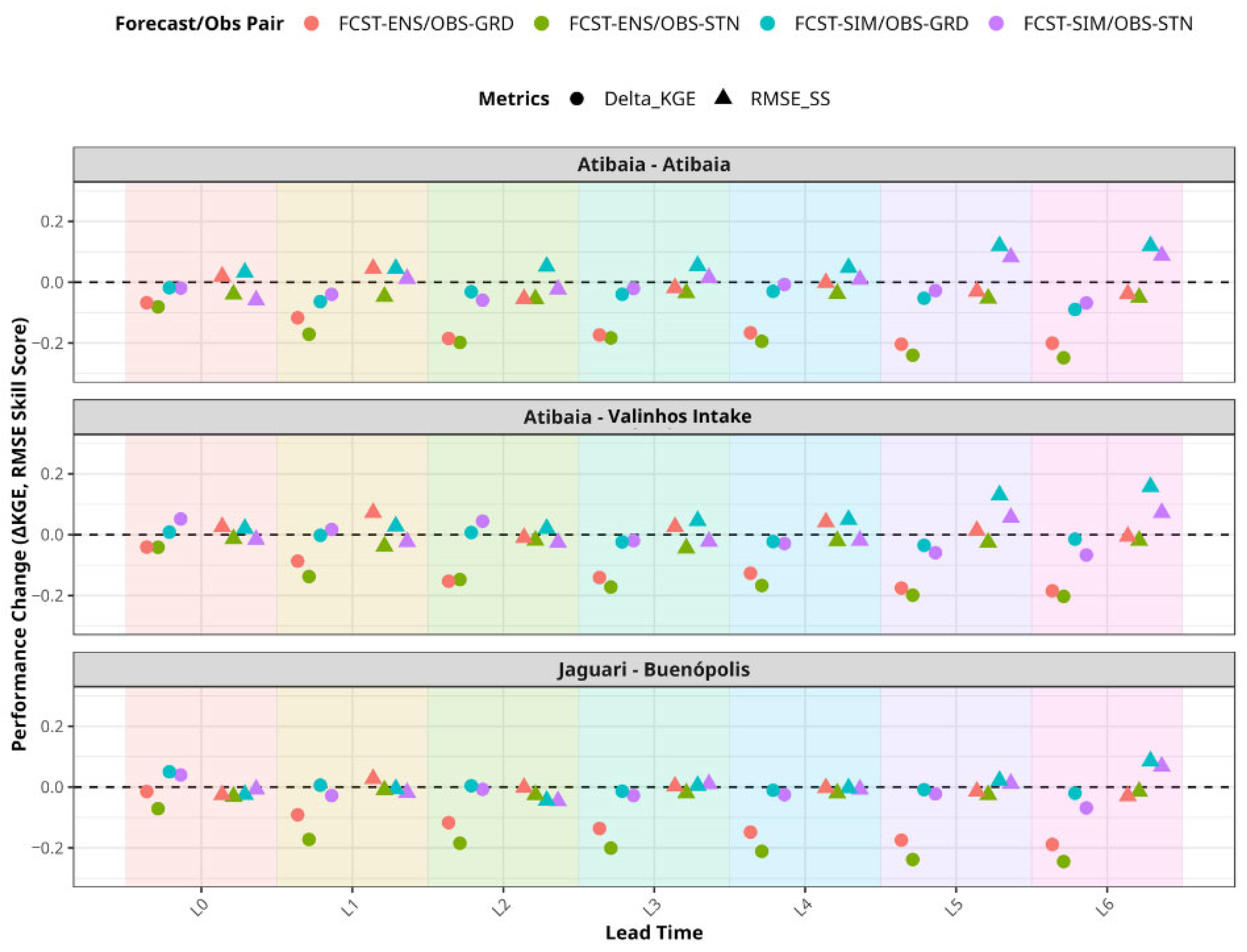
In the second step, the performance of the bias-correction methods was evaluated using continuous metrics that measure the difference between forecasts and observations. The primary metric used was the Kling-Gupta Efficiency (KGE), which provides a generalized measure of model performance by combining correlation, bias, and variability into a single index. This allows a comprehensive assessment of how well the corrected forecasts reproduce the observed values [41].

The KGE is defined in Equation (10):

$$KGE = 1-\sqrt{{\left(r-1\right)}^2 + {\left(\alpha - 1\right)}^2 + {\left(\beta -1\right)}^2}$$

(10)

where

r = correlation between forecast and observation (temporal agreement)

α = σ_f/σ_o = variability ratio between forecast and observed standard deviations

β = μ_f/μ_o = bias ratio between forecast and observed means

Values of α and β equal to 1 indicate agreement between the forecast and observations in terms of relative variability and mean, respectively, while (r = 1) indicates perfect linear association.

The KGE components were evaluated for the raw and bias-corrected forecasts for each basin, forecast–observation pairing, and forecast lead time. Changes in each component were calculated to identify the specific aspects of forecast performance affected by bias correction. An improvement in (r) indicates stronger temporal association with the observations, whereas values of β and α closer to 1 indicate improved agreement in the mean and relative variability, respectively. This decomposition was used to determine whether changes in KGE resulted primarily from improvements in correlation, mean bias, or variability, and to identify potential trade-offs among these components.

The effectiveness of the bias-correction methods was evaluated using the change in KGE, as shown in Equation (11):

ΔKGE = KGE_Cor − KGE_Raw

(11)

where KGE_Cor represents the relationship between the corrected forecast and the observations, and KGE_Raw represents the relationship between the raw forecast and the observations.

To express the magnitude of forecast errors in physical units (mm day⁻¹), the Root Mean Square Error (RMSE) was also calculated. Additionally, the RMSE skill score [24] was used to quantify the improvement introduced by the bias-correction methods relative to the raw forecasts, as shown in Equation (12):

$$\mathrm{SSRMSE} = 1 - {\displaystyle \frac{RMS{E}_{Cor}}{RMS{E}_{Raw}}}$$

(12)

where RMSE_Cor corresponds to the RMSE of the corrected forecasts and RMSE_Raw corresponds to the RMSE of the raw forecasts.

Values of the skill score close to 1 indicate a strong improvement relative to the raw forecasts. Values close to 0 indicate little or no improvement, while negative values indicate that the correction method degraded the forecast performance.

3. Results

3.1. Raw Forecast Categorical Performance

Overall, Figure 2 reveals clear differences in the predictability of dry and wet events between the two forecasting systems, and these differences are consistent across all three basins. In general, FCST-ENS exhibited superior categorical performance, with consistently higher ACC and CSI values and lower FAR values when evaluated against both observational datasets. In addition, FCST-ENS demonstrated greater temporal stability, characterized by a gradual reduction in skill with increasing lead time. In contrast, FCST-SIM generally produced higher POD values, particularly at shorter lead times, but exhibited a more rapid degradation in performance at longer lead times.

The comparison among forecast–observation pairs also highlights the sensitivity of categorical verification to the observational reference dataset. This sensitivity is especially evident for FCST-ENS, for which noticeable differences between OBS-STN and OBS-GRD can be observed in ACC, CSI, and POD. In general, FCST-ENS evaluated against OBS-GRD exhibited higher ACC and CSI values, whereas FAR values were slightly higher than those obtained using OBS-STN as reference. A similar pattern was observed for FCST-SIM, although the differences between observational datasets were generally smaller and less variable across lead times than those found for FCST-ENS.

The overall behavior was remarkably consistent across the three basins, suggesting that forecast-system characteristics exert a stronger influence on categorical performance than basin-specific factors.

3.2. Dry/Wet Occurrence Correction

Figure 3 presents the results of the exact McNemar test, expressed as odds ratios in a heat map. Red values indicate a greater number of cases in which the correction changed an incorrect raw prediction into a correct prediction than the reverse. Stars indicate Holm-adjusted p-values within each lead time (* p < 0.05, ** p < 0.01, *** p < 0.001). Open diamonds indicate cases in which both discordant counts were zero (b = 0 and c = 0), resulting in an undefined odds ratio, whereas filled diamonds indicate infinite odds ratios resulting from c = 0, with the displayed values capped at 10 for visualization.

Overall, the results indicate that the correction methods tended to provide greater improvements for forecast–observation pairs involving FSCT-SIM, particularly for the FSCT-SIM/OBS-GRD pairing. For this pairing, improvements were observed across the three basins and for most correction methods over approximately five lead times, with statistically significant differences becoming more frequent at the final three lead times. In contrast, the improvements observed for the FSCT-ENS pairings were more moderate and less consistent, varying among basins, correction methods, and lead times.

The behavior of LR-Seasonal is particularly noteworthy. For this method, 10 cases resulted in b = 0 and c = 0, represented by open diamonds in Figure 3. These cases indicate that the correction did not alter the classification relative to the raw forecast: no observations changed from incorrect to correct, and no observations changed from correct to incorrect. These cases occurred across the three basins and the three forecast–observation pairings considered (FSCT-SIM/OBS-GRD, FSCT-SIM/OBS-STN, and FSCT-ENS/OBS-GRD), particularly at lead times L0, L1, L3, and L4.

Conversely, LR-Seasonal produced four cases with an infinite odds ratio (c = 0), represented by filled diamonds in Figure 3. In these cases, at least one incorrect raw prediction was corrected (b > 0), while no initially correct prediction became incorrect. The odds ratios for these cases are displayed as 10 due to the imposed visualization cap. These cases occurred across the three basins for the gridded-observation pairings involving both forecasting datasets and were concentrated at the latest lead times, L5 and L6.

Figure 4 shows a heat map of the differences between categorical verification metrics from the corrected and raw forecasts, averaged across the seven forecast lead times. To ensure a consistent interpretation in which positive values always denote improved performance, differences were calculated as corrected minus raw for POD, CSI, and ACC, and as raw minus corrected for FAR. Positive values (red shades) therefore indicate an increase in POD, CSI, or ACC, or a decrease in FAR, while negative values (blue shades) indicate deterioration in any of the four metrics.

Statistical significance, assessed via bootstrap 95% confidence intervals, is overlaid on the same cells: a filled circle marks a significant improvement (confidence interval excludes zero and the difference is positive), and a cross marks a significant decline (confidence interval excludes zero and the difference is negative). Cells whose confidence interval includes zero carry no marker, indicating no statistically significant difference.

Overall, the figure shows the trade-off between POD and FAR across the three basins, all methods, and the four pairings. The FCST-ENS tends to show gains in POD and declines in FAR, indicating that the model becomes drier after correction, with an exception in the Jaguari basin, where FCST-ENS/OBS-STN improvements occur across all four metrics. The FCST-SIM, on the other hand, tends to show the opposite pattern, with POD decreasing and FAR increasing after correction, indicating that the corrected model tends to predict more wet days than the raw one.

The range of the mean differences between raw and corrected forecasts is similar across metrics, from a decrease of −0.3 points in POD for LR-Seasonal (FCST-SIM/OBS-GRD, Atibaia basin) to an increase of +0.2, where the largest gains are more evident for POD and FAR, though for different FCST/OBS pairings.

The four metrics used to assess the four methods are, in general, similar, making it difficult to identify which method performs best overall. It is easier, however, to identify the worst-performing method: LR-Seasonal, which resulted in POD = 0 and CSI = 0 for the Atibaia basin (FCST-SIM/OBS-GRD) at lead times L1 and L4 (Figure A1).

An exact permutation test was applied to the differences between raw and corrected metrics across the seven lead times, for each method, FCST/OBS pairing, and basin. After Holm adjustment of the p-values across the four methods for each metric, no statistically significant differences were found, making it difficult to determine which method performs best statistically.

Figure 5 presents the results of the descriptive multi-metric ranking analysis used to compare the relative performance of the four occurrence-correction methods. For each basin and forecast–observation pairing, the performance of the four methods was first ranked separately for POD, CSI, ACC, and FAR using the values averaged across the seven forecast lead times. These four metric-specific ranks were then averaged to obtain an overall rank for each correction method, with lower values indicating better overall performance across the four categorical verification metrics. The figure therefore shows the distribution of the 12 overall rank values obtained for each method across the three basins and four forecast–observation pairings. Individual overall-rank values are represented by gray points, and red diamonds indicate their average.

As shown in Figure 5, HBLR-AR1 had the lowest mean overall rank (1.88), followed by HBLR-Seasonal (2.50), LR-AR1 (2.79), and LR-Seasonal (2.83). Thus, based on the combined ranking of POD, CSI, ACC, and FAR, HBLR-AR1 showed the best relative overall performance among the four correction methods, while the Bayesian methods generally achieved lower mean ranks than the frequentist methods.

3.3. Bias-Correction Performance Using the Complete Chronological Series

Figure 6 presents the changes in forecast performance after applying QDM bias correction to the complete chronological series across forecast lead times and basins, evaluated using ΔKGE and the RMSE skill score. The results are restricted to the independent test dataset. Positive values indicate improvement relative to the raw forecasts, whereas negative values indicate degradation.

Overall, the results indicate that the effect of QDM was dependent on the verification metric, forecast lead time, basin, and forecast–observation pairing. Regarding metric dependence, across the three basins, improvements in RMSE were frequently accompanied by reductions in KGE, indicating that a reduction in the magnitude of forecast errors does not necessarily translate into improved overall forecast efficiency. This difference arises from the distinct aspects of forecast performance represented by the two metrics: RMSE evaluates the magnitude of forecast errors, whereas KGE combines correlation, mean bias, and relative variability. Therefore, QDM can reduce forecast errors while simultaneously producing changes in one or more KGE components that result in a lower overall KGE. The contribution of these components is examined separately below. An exception was observed for the Atibaia– Valinhos Intake basin and the FCST-SIM/OBS-GRD pairing, for which both metrics showed modest improvements at the first three lead times.

The dependence on forecast lead time is evident from the larger RMSE improvements observed at longer lead times. Across the three basins, the largest improvements occurred at L5 and L6, with RMSE skill scores ranging approximately from 0.10 to 0.18. These lead times also generally exhibited larger discrepancies between the raw forecasts and observations. This pattern suggests an association between the magnitude of the initial forecast errors and the potential gain from QDM, with larger raw errors providing greater scope for reduction after bias correction. However, this relationship was not uniform across all forecast–observation configurations or verification metrics.

The dependence on the forecast–observation pairing is also evident in the magnitude of the RMSE skill improvements. Gains were more pronounced for FCST-SIM across the three basins, particularly for the FCST-SIM/OBS-GRD pairing. In contrast, the FCST-ENS pairings generally showed moderate to negligible changes in RMSE skill, with the FCST-ENS/OBS-GRD configuration showing the most evident improvement among the ensemble-based pairings.

Differences among basins were also observed. The Jaguari basin showed mostly marginal to moderate improvements across the four forecast–observation pairings. Valinhos Intake exhibited improvements in both RMSE and KGE for three pairings: FCST-ENS/OBS-GRD, FCST-SIM/OBS-GRD, and FCST-SIM/OBS-STN. In contrast, the Atibaia basin showed a similar pattern of RMSE improvement across the configurations, but these improvements were not accompanied by corresponding improvements in KGE. These results further demonstrate that the effect of QDM was not spatially uniform and depended on the specific basin and forecast–observation configuration.

To further investigate the contrasting responses of RMSE and KGE, the KGE was decomposed into its three constituent components: the correlation coefficient (r), bias ratio (β), and variability ratio (α). The decomposition was performed for the raw and QDM-corrected forecasts for each basin, forecast–observation pairing, and lead time. The correlation component was evaluated based on changes in r, whereas the bias and variability components were evaluated according to their distance from their ideal value of 1. Thus, an increase in r, or a reduction in ∣β − 1∣ or ∣α − 1∣, represents an improvement in the corresponding component.

Table 6. Mean change in KGE components after bias correction.

	Δr	Δα (Skill)	Δβ (Skill)	ΔKGE
Atibaia
ENS/GRD	−0.004 (2/7)	−0.148 (0/7)	−0.158 (0/7)	−0.173 (0/7)
ENS/STN	−0.019 (0/7)	−0.087 (0/7)	−0.262 (0/7)	−0.185 (0/7)
SIM/GRD	0.008 (6/7)	−0.154 (0/7)	−0.087 (0/7)	−0.046 (0/7)
SIM/STN	−0.016 (1/7)	−0.069 (1/7)	−0.075 (1/7)	−0.034 (0/7)
Valinhos Intake
ENS/GRD	0.001 (4/7)	−0.158 (0/7)	−0.153 (0/7)	−0.160 (0/7)
ENS/STN	−0.018 (0/7)	−0.083 (0/7)	−0.216 (0/7)	−0.169 (0/7)
SIM/GRD	0.008 (6/7)	−0.094 (0/7)	−0.045 (3/7)	−0.012 (2/7)
SIM/STN	−0.006 (2/7)	−0.007 (5/7)	−0.064 (3/7)	−0.009 (3/7)
Jaguari
ENS/GRD	−0.007 (1/7)	−0.097 (1/7)	−0.147 (0/7)	−0.126 (0/7)
ENS/STN	−0.021 (0/7)	−0.110 (0/7)	−0.263 (0/7)	−0.192 (0/7)
SIM/GRD	−0.003 (1/7)	−0.015 (3/7)	−0.015 (3/7)	0.001 (3/7)
SIM/STN	−0.013 (0/7)	−0.017 (3/7)	−0.059 (1/7)	-0.020 (1/7)

summarizes the changes in the KGE components and provides additional insight into the mechanisms underlying the changes in KGE after QDM correction. The values in parentheses indicate the number of lead times, out of seven, for which the corresponding component showed an improvement. The decomposition indicates that the reduction in KGE observed for most configurations was primarily associated with deterioration in the α and β components. The mean changes in α were negative for all basin and forecast–observation configurations, ranging from −0.007 to −0.158, while the mean changes in β were also negative in all cases, ranging from −0.015 to −0.263. In particular, the ENS/STN and ENS/GRD configurations generally exhibited the largest reductions in both components, with no improvement in β across any of the seven lead times. These results indicate that, although QDM reduced the magnitude of the forecast errors in several configurations, it did not consistently improve the agreement between forecast and observed variability or mean precipitation, which contributed to the reductions in KGE.

In contrast, the response of the correlation component was considerably smaller and more variable among the configurations. The mean change in r ranged from −0.021 to 0.008. For the SIM/GRD pairing, r increased at six of the seven lead times in both Atibaia and Valinhos Intake, with a mean increase of 0.008. However, this improvement in correlation was not sufficient to offset the deterioration in the α and β components, and KGE still decreased by 0.046 and 0.012, respectively. This provides a clear example of why improvement in one KGE component does not necessarily result in an overall KGE improvement.

The Valinhos Intake SIM/STN configuration provides another example of the more balanced response of the KGE components. Although the mean changes in r, α, and β were negative, the α component improved at five of the seven lead times, while β improved at three. Nevertheless, the mean KGE change remained slightly negative (−0.009). In contrast, the Jaguari SIM/GRD configuration was the only case in which the mean KGE showed a marginal positive change (+0.001), although the mean changes in r, α, and β were close to zero.

Overall, the decomposition demonstrates that the frequent disagreement between RMSE and KGE was not primarily related to changes in correlation but rather to changes in the mean and variability components of KGE. QDM therefore showed an ability to reduce error magnitude without consistently improving the distributional characteristics represented by α and β. These results reinforce that the effect of bias correction should be interpreted in relation to the specific verification metric, as improvement in RMSE does not necessarily imply improvement in the individual components or the overall KGE.

4. Discussion

The combined assessment of categorical verification metrics, statistical testing, and multi-metric ranking provides a consistent picture of the benefits and limitations of logistic-regression-based occurrence correction for the detection of dry events. The raw forecasts showed systematic differences in categorical performance between the two forecast sources. In particular, the FCST-SIM pairing generally exhibited lower ACC and CSI than the FCST-ENS pairing across the three basins and forecast lead times. Consistent with these differences, the McNemar exact test provided stronger evidence of changes in classification skill after occurrence correction for the FCST-SIM pairing than for the FCST-ENS pairing. These results suggest that the potential benefit of occurrence correction is partly dependent on the initial categorical characteristics of the raw forecasts.

The changes in the categorical metrics further showed a systematic trade-off between dry-event detection and false alarms. For the FCST-ENS pairing, improvements in POD were generally accompanied by degradation in FAR, whereas the FCST-SIM pairing showed the opposite pattern, with degradation in POD generally accompanied by improvements in FAR. These contrasting responses were consistent with the characteristics of the corresponding raw forecasts. An exception was observed for the FCST-ENS/OBS-STN pairing in the Jaguari basin, where the raw forecast exhibited a comparatively higher FAR than the other basins. This characteristic may have provided greater scope for the occurrence correction to improve the balance between dry-event detection and false alarms, resulting in simultaneous improvement in POD and FAR. Nevertheless, the McNemar results indicate that these improvements should be interpreted with caution, as the changes in paired classification were not consistently statistically significant.

The comparison of the four correction methods also indicates that their performances were relatively similar across the three basins and four forecast–observation pairings, making the identification of a single superior method less straightforward. Nevertheless, the results provide useful evidence for excluding methods with less consistent behavior. The LR-Seasonal method showed the least favorable overall performance, including cases in which the correction produced no change in classification relative to the raw forecast and cases with no improvement in CSI and POD. For example, in the Atibaia basin, CSI and POD showed no improvement at lead times L1 and L4. When considered together with the McNemar results, including the cases in which the correction did not alter the classification relative to the raw forecast, these results suggest that the performance of LR-Seasonal was not sufficiently consistent across the experimental conditions to support its selection as the preferred correction method.

The descriptive multi-metric ranking provided additional evidence for selecting among the remaining methods. HBLR-AR1 showed the most favorable overall performance across the categorical metrics and experimental configurations, followed by HBLR-Seasonal, LR-AR1, and LR-Seasonal. This result was also consistent with the McNemar analysis, in which HBLR-AR1 produced the highest number of cases showing an improvement in classification relative to the raw forecast. Across the 84 combinations of lead time, basin, and forecast–observation pairing, HBLR-AR1 showed improvements in 30 cases, compared with 23 for HBLR-Seasonal, 22 for LR-AR1, and 16 for LR-Seasonal. Although these results do not establish statistically significant differences between the correction methods themselves, their consistency across the complementary analyses supports HBLR-AR1 as the most favorable method under the experimental conditions considered.

Finally, the choice of correction methods should also consider computational cost, particularly for potential operational applications. The frequentist models were substantially faster to calibrate, with the complete calibration for one basin, four forecast–observation pairings, seven lead times, and two correction configurations requiring less than one minute. In contrast, the Bayesian models required more than three hours for the equivalent calibration, reflecting the additional computational burden associated with MCMC sampling. This difference is relevant for operational implementation, although the computational requirements of an operational system would depend on the number of models retained and the frequency of recalibration. The identification of a preferred correction method and forecast source could substantially reduce this computational burden by limiting the number of configurations that need to be calibrated. In this regard, the limited statistical evidence of improvement for the FCST-ENS pairing in the McNemar analysis suggests that the operational benefit of applying occurrence correction to the ensemble forecast should be carefully weighed against its computational cost.

Applying QDM to correct forecast magnitude showed a clear dependence on the verification metric and forecast lead time. Although improvements in RMSE were observed across several configurations, these improvements were not consistently accompanied by improvements in KGE. The decomposition of KGE further indicated that the deterioration was primarily associated with the variability and bias components rather than with changes in correlation. One possible technical explanation for this behavior is the imposed upper limit on the multiplicative correction factor (ratio.max = 2). By constraining large correction factors, this setting may limit the extent to which QDM can adjust large differences between the forecast and observed precipitation distributions and, consequently, may affect the corrected mean and variability. Therefore, part of the observed deterioration in the α and β components cannot be attributed exclusively to the QDM method itself and may also be influenced by the selected ratio.max value. However, because a sensitivity analysis using higher values of ratio.max was not performed, the magnitude of this potential effect cannot be quantified, and this explanation should therefore be regarded as a possible technical limitation of the present implementation rather than a demonstrated cause of the observed KGE deterioration.

Across the five correction configurations evaluated in this study—four for occurrence correction and one for precipitation-magnitude correction—two common patterns emerged. First, the forecast–observation pairing had an important influence on the results. The effectiveness of the correction methods varied depending on the forecast and observation datasets being paired, indicating that the characteristics and magnitude of the differences between forecasts and observations play an important role in how much the statistical correction methods can learn and correct. Thus, the greater the variability or discrepancy between the forecast and observation, the greater the potential for the correction methods to modify the forecasts and produce measurable improvements.

Considering specifically the discrepancies between the forecasts and the station-based precipitation, uncertainties in the spatial representation of the observations may also contribute to the differences between the forecasts and observations. In this study, basin-average precipitation from the rain-gauge observations was estimated using the arithmetic mean of the available stations. Although this approach provides a simple representation of basin-average precipitation, it may not fully capture the spatial variability of precipitation across the basin, particularly when only a limited number of rain gauges are available. This limitation may be particularly relevant in the study region, where precipitation is frequently characterized by convective events with substantial spatial variability. Consequently, part of the apparent discrepancy between the spatial forecast products and the station-based observations, and therefore part of the forecast error attributed to the models, may reflect uncertainties in the spatial representation of the observational reference itself.

Second, for both occurrence and magnitude correction, the improvements were generally more pronounced at later forecast lead times. This pattern may be related to the increasing differences between forecast and observed conditions with lead time, which provide greater scope for the correction methods to identify and adjust systematic discrepancies. Together, these results suggest that the effectiveness of statistical correction depends not only on the correction method itself but also on the magnitude and characteristics of the forecast–observation differences that the method is able to learn from the calibration data.

5. Conclusions

This study evaluated the performance of two precipitation forecasting systems using two observational reference datasets across three basins in the state of São Paulo and assessed the effectiveness of two bias-correction approaches: Quantile Delta Mapping (QDM) for precipitation amounts and logistic-regression-based methods for dry/wet occurrence correction.

Overall, the results demonstrate that the effectiveness of statistical post-processing depends strongly on the characteristics of forecast–observation pairing. For occurrence correction, logistic-regression-based methods modified the categorical classification of the raw forecasts and, in several configurations, improved specific aspects of dry-event prediction. However, the magnitude and direction of these changes varied among forecast sources, observation datasets, basins, and lead times. The results also revealed a trade-off between dry-event detection and false alarms, highlighting that improvements in one categorical metric do not necessarily imply simultaneous improvements in all aspects of forecast classification. Among the methods evaluated, HBLR-AR1 provided the most consistent overall performance, whereas LR-Seasonal showed the least favorable and least consistent behavior. Nevertheless, the relatively small differences among the correction methods indicate that method selection should consider not only predictive performance but also the statistical evidence supporting the improvement and the computational cost of model calibration.

For precipitation amounts, QDM showed strongly metric-dependent performance. Although improvements in RMSE skill score were observed, particularly at longer lead times, consistent gains in ΔKGE were not achieved. The KGE results therefore indicate that reductions in error magnitude do not necessarily translate into simultaneous improvements in other dimensions of forecast quality, such as temporal correlation and variability. The stronger improvements observed at longer lead times across both occurrence and magnitude correction further suggest that the magnitude and characteristics of forecast–observation discrepancies play an important role in determining the potential benefit of statistical correction.

From a practical perspective, although the Bayesian occurrence-correction methods required substantially greater computational time for calibration than the frequentist approaches, this difference does not necessarily represent a limitation for operational implementation. In practice, model calibration can be performed at predefined intervals rather than for every forecast cycle, allowing the computationally intensive calibration step to be scheduled independently of the operational forecasting process. For example, periodic recalibration at six-month intervals could allow the models to incorporate newly available forecast–observation pairs while avoiding interference with the operational forecast production. As the calibration dataset progressively increases with the inclusion of new observations, the estimated model parameters may also become more stable over time.

Future developments may benefit from hybrid post-processing approaches that combine occurrence and magnitude correction while accounting for the different characteristics of precipitation occurrence and intensity. Further research should also investigate whether the improvements identified at the precipitation-forecast level propagate to hydrological predictions. Although improving precipitation forecasts is an important intermediate objective, the ultimate practical value of bias correction lies in its capacity to improve downstream applications, particularly streamflow forecasting and water-resources management.