A Data-Driven Approach to Close the Water Balance of a Cascaded Multiple Reservoir–Lake System

Abstract

This study presents a data-driven methodology to develop and close the continuous water balance of a cascaded hydrological system consisting of two upstream regulating reservoirs and a downstream lake. The analysis is based on monthly hydrometeorological and hydrographic data for the period 1998–2024. A baseline water balance model using raw measured data was first implemented, followed by two bias correction approaches based on multiple linear regression coefficient estimation. The first approach applies uniform coefficients across all months, while the second accounts for seasonal variability by estimating coefficients only for the December–May period, when systematic errors are most pronounced. Model performance was evaluated using calibration (1998–2017) and validation (2018–2024) periods, with Nash–Sutcliffe efficiency (NSE) and residual diagnostics used as evaluation metrics. The baseline model showed substantial cumulative deviations due to systematic errors (NSE: −0.28 and −5.13 for the two reservoirs and −18.70 for the lake), confirming the need for bias correction. Both correction approaches significantly improved model performance, with NSE values up to 0.89 for reservoirs and 0.83–0.86 for the lake during calibration. In validation, the seasonally adjusted model performed more stably in simulating water levels for Lake Velence (NSE = 0.72) than the uniform coefficient model (NSE = 0.60), particularly under extreme hydrological conditions. Residual analysis further indicated improved independence and homoscedasticity when seasonal structure was considered. The results demonstrate that water balance closure in the system is affected by distributed errors across multiple components rather than a single dominant source. The proposed methodology provides a practical, scalable framework for reconstructing consistent water balance time series in data-limited, regulated systems and supports the development of water management scenarios.

1. Introduction

Lakes and reservoirs constitute essential freshwater resources, supporting municipal, industrial, agricultural, and ecological functions [1]. They represent a major component of the global hydrological system, storing a significant portion of the Earth’s accessible surface freshwater and providing critical ecosystem services [2]. Due to their multifunctional role and sensitivity to both climatic variability and human intervention, their sustainable management is increasingly important [3].

A key requirement for effective water resources management is the ability to understand past water level dynamics and reliably predict future water availability [4,5]. The water balance equation provides a fundamental framework for this purpose by linking changes in storage to inflows, outflows, and an aggregated error term [6]. In theory, the long-term application of the water balance requires that the error term has a zero mean, implying that only random measurement errors are present and that they cancel out over time [7]. In practice, however, water balance components are affected by both random and systematic errors, resulting in persistent imbalances that accumulate over time and ultimately compromise the reliability of water balance models [8].

Addressing these imbalances is therefore a central challenge in hydrology [9]. Researchers have proposed various approaches, including integrating multiple data sources [10], applying physically based or data assimilation methods [11], and redistributing residual errors among water balance components [12]. While these methods can improve consistency, they are often computationally demanding, data-intensive, or difficult to apply in operational water management contexts [13,14].

In parallel, data-driven approaches, such as multiple linear regression (MLR), have been widely used in hydrology due to their simplicity, transparency, and ability to identify relationships between variables [15,16,17]. However, their application has primarily focused on modeling hydrological responses, such as rainfall–runoff relationships, rather than directly addressing the closure of water balance equations. Additionally, most studies focus on individual lakes or reservoirs, whereas few examine cascaded systems with multiple connected reservoirs and lakes. In such systems, errors may propagate both temporally and spatially, further complicating the achievement of a consistent system-wide water balance [18].

Lake Velence and its upstream regulating reservoirs represent a typical example of such a cascaded system [19]. Reservoir operations, regulated inflows, and anthropogenic pressures exert a strong influence on the lake, while existing water balance calculations exhibit significant systematic errors and rely partly on retrospective adjustments [20]. These limitations restrict the direct use of observed and calculated time series for long-term modeling and scenario analysis.

Therefore, there is a need for a practical, operationally applicable methodology that enables consistent reconstruction and closure of the water balance in interconnected and regulated systems while remaining applicable in data-limited operational contexts. This study addresses this need by proposing a data-driven bias correction framework based on multiple linear regression, applied directly to the water balance components of a cascaded reservoir–lake system. In contrast to previous applications of regression methods, which typically focus on hydrological response modeling, the proposed approach aims to close the system’s continuous monthly water balance. Two different bias correction model formulations are evaluated, including one that explicitly accounts for seasonal patterns in water balance errors, thereby addressing the temporal structure of systematic biases.

The objective of this study is to develop a data-driven methodology for constructing and closing the continuous water balance of a cascaded reservoir–lake system using long-term monthly data. The study first constructs a baseline water balance model using raw measured data, followed by two bias correction approaches based on multiple linear regression coefficient estimation. The performance of these models is evaluated through calibration and validation, with particular attention to the role of seasonal error patterns. The resulting closed water balance provides a consistent basis for subsequent water management scenario analysis.

2. Literature Review

2.1. Lakes, Reservoirs, and Water Resources Management

Lakes and reservoirs are fundamental components of the hydrological system and play a critical role in water resources management. Lakes represent a major storage of freshwater, as they store the largest liquid water mass on the terrestrial surface [2,21]. At the same time, reservoirs actively regulate hydrological processes by redistributing river flow in space and time [5,22]. Given their importance, water managers must understand the availability and sustainability of these systems, for which water balance modeling provides a fundamental analytical framework [6].

Fluctuations in lake water levels are particularly informative indicators of both climatic variability and anthropogenic impacts [23]. Identifying the drivers behind these fluctuations is therefore crucial for effective lake management [24]. Consequently, water balance modeling has become a widely used and essential tool for analyzing lake dynamics and supporting water management decisions [18]. Its relevance is further demonstrated across a range of applications, including agricultural water management [25], flood and drought risk mitigation through reservoir regulation [5], climate change impact assessment and scenario analysis [26,27], and the analysis of lake level dynamics and their driving mechanisms [18,24].

2.2. Water Balance Calculation, Uncertainty, and Error Sources

The water balance provides the conceptual foundation for hydrological analysis; however, its practical application involves significant uncertainties [7]. Although the concept is straightforward, water budgets are often difficult to determine accurately due to limited data availability and measurement precision [6]. A persistent issue in the literature reveals that errors in individual water balance components are often not analyzed in sufficient detail, despite their substantial influence on results [7]. Studies of large lake systems, such as Lake Victoria [23], highlight that the primary objective of water balance modeling is to explain major water level fluctuations. However, due to limited observational data, these estimates often disclose considerable uncertainty. Similar challenges arise in reservoir systems, where water balance estimation may become ill-posed when key fluxes are not directly measured [28].

Further complications arise from sparse monitoring networks, particularly in large or remote basins, which limit the reliability of precipitation and other input data [8]. In addition, modeling errors can propagate over time due to the inherent inertia of large water bodies, thereby amplifying inaccuracies in long-term simulations [24]. These factors demonstrate that uncertainties in water balance modeling are both structural and data-driven and must be explicitly addressed to ensure reliable interpretation.

2.3. Methods for Closing the Water Balance

Given their inherent uncertainties, various methods have been developed to achieve closure in water balance calculations and improve model reliability. One common approach introduces additional constraints, thereby reducing errors in individual water balance components and improving overall system consistency [9]. More advanced techniques focus on analyzing and redistributing residual errors, such as precipitation decorrelation and residual redistribution methods, which aim to identify and correct systematic biases in the water balance [12]. Calibration-based approaches are also widely applied, in which model parameters are adjusted to achieve the best agreement between observed and simulated water level changes [16].

In addition, probabilistic frameworks can explicitly represent uncertainties and biases in input data, thereby enabling a more consistent reconciliation of multiple data sources [29]. When data availability is limited, structural approaches that constrain hydrological models using available observations can help address ill-posed water balance problems [28].

Data assimilation techniques aim to achieve full water balance closure by integrating ground-based measurements with Earth observation data. They ensure consistency with governing equations and correct biases in individual components, for example, through Bayesian hierarchical modeling [11]. Overall, these approaches demonstrate that achieving water balance closure typically requires a combination of statistical, physical, and data-driven methods.

2.4. Application of Multiple Linear Regression in Closing the Water Balance

A simpler and widely used data-driven approach for bias correction and supporting water balance closure is multiple linear regression (MLR). Regression-based methods enable the identification and correction of systematic biases in water balance components by relating them to observable variables. The main advantage of MLR lies in its simplicity and transparency, making it well suited for identifying relationships between model residuals and explanatory variables [16]. Such approaches can enhance water balance modeling by providing additional insight into system behavior and enabling data-driven correction of errors [16]. Regression analysis has examined key water balance components to support water resource management decisions across various lake systems [16,30,31].

The application of MLR is particularly relevant in cases where input data require adjustment, as demonstrated in studies that bias-correct climate model outputs before their use in water balance simulations [23]. However, the use of regression methods requires careful model specification and validation, including assessing parameter significance and verifying model robustness [32,33].

2.5. Research Gap and Novelty

To address limited observations and measurement errors, previous studies have proposed a range of approaches, including data assimilation techniques, probabilistic frameworks, and residual redistribution methods, to improve consistency among water balance components [9,11,12,29]. While these methods have proven effective in reducing uncertainty, they are often computationally complex, data-intensive, or difficult to implement in operational water management contexts.

At the same time, regression-based methods, particularly MLR, have been widely applied in hydrology due to their simplicity, transparency, and ability to capture relationships between hydrological variables [16,30]. However, their application has largely focused on modeling hydrological responses (e.g., rainfall–runoff relationships) rather than directly addressing water balance closure problems. Only limited examples exist where regression approaches support water balance consistency or correct individual components [31], and even in these cases, their role remains secondary rather than central.

Another limitation in the literature is the lack of studies on cascaded water systems with multiple connected reservoirs and lakes. Most existing work focuses on single lakes or reservoirs, while interconnected systems introduce additional complexity due to error propagation and dependency between upstream and downstream components. As demonstrated in large lake systems, inaccuracies can propagate over time due to system inertia [24]. However, this issue is even more critical in cascaded systems, where errors transfer spatially as well.

Studies that explicitly consider regulated systems highlight the importance of operational rules and human interventions. For instance, in the Lake Victoria system, dam management scenarios have been shown to exert a stronger influence on water levels than climate forcing alone [26].

Therefore, this study addresses these gaps by proposing a data-driven bias correction framework based on MLR, applied directly to the water balance components of a cascaded reservoir–lake system. The study evaluates two different MLR-based model formulations: the first models the system continuously throughout the year. In contrast, the second explicitly accounts for seasonal patterns observed in water balance errors.

3. Site Description and Data

3.1. Study Area

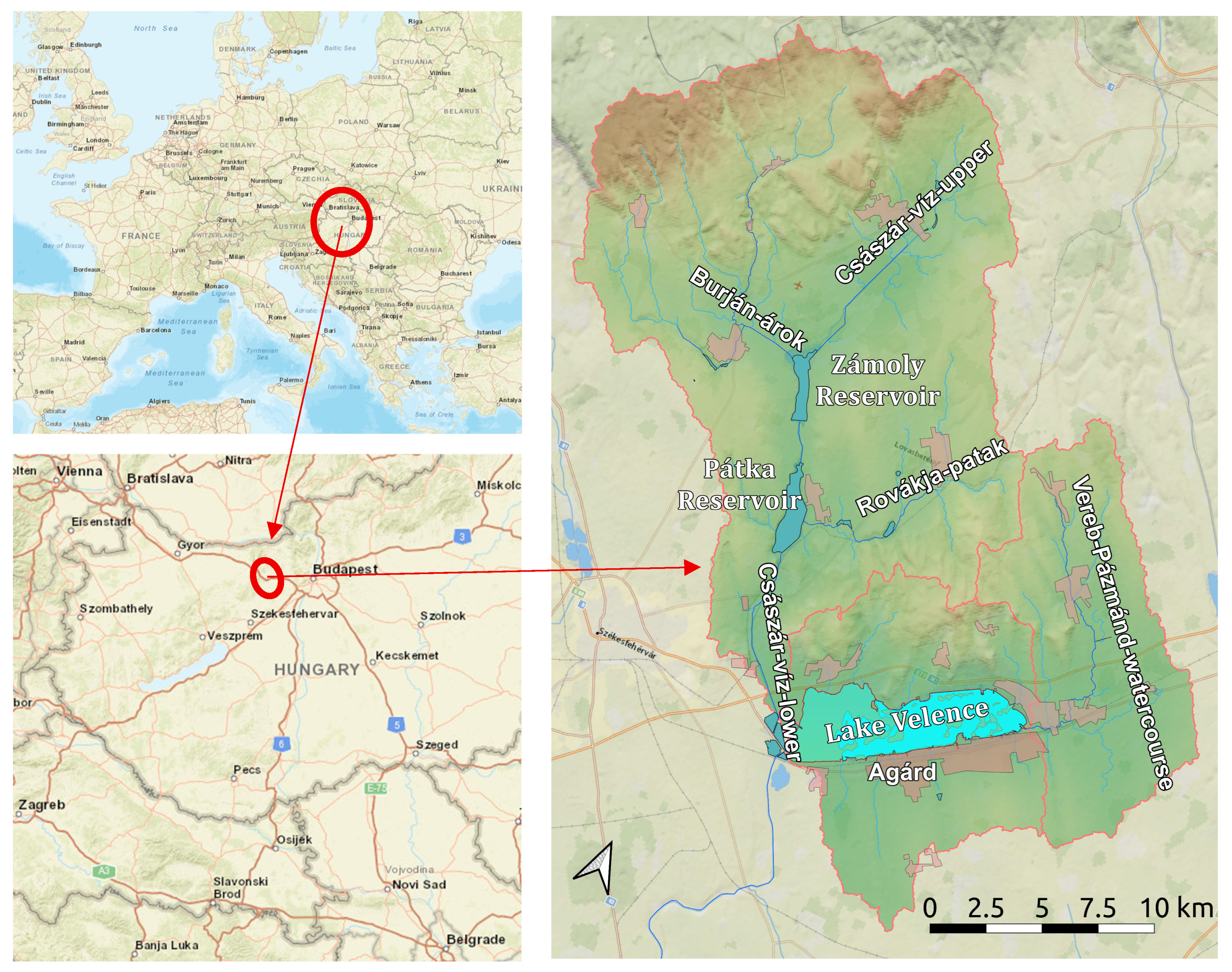
Lake Velence is a shallow lake located in Central Hungary. The total catchment area (including the lake) is 602.3 km², covering the south-eastern slope of the Vértes Mountains, the northern part of Mezőföld, and the Velence Mountains. Upper Carboniferous granite forms most of the Velence Mountains, while Upper Eocene andesite volcanics also occur in the north-northeastern part of the mountain range. Mesozoic carbonates are present in the north-northwestern part of the watershed, whereas Pannonian and Quaternary formations dominate in the central and southern parts [34].

Hydrologically, the catchment consists of three main sub-basins. The largest (383 km²) is the Császár-víz watershed, whose upper ~75 km² karstic area is partially inactive. The second main tributary is the Vereb–Pázmándi watercourse (105 km²), while the remaining direct catchment of the lake covers 114.3 km². Among the inflows of the lake, only the Császár-víz is a permanent stream.

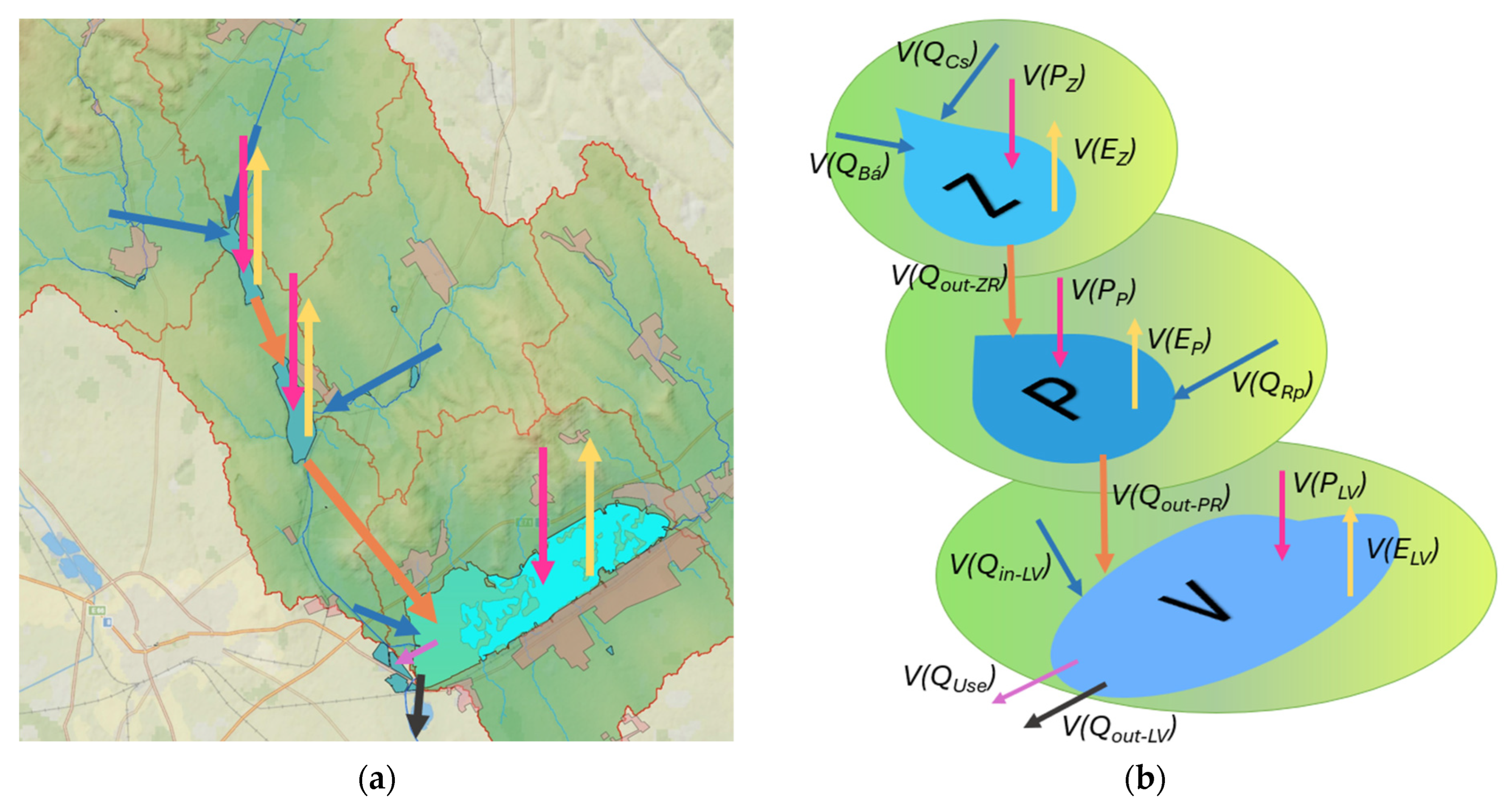
The hydrological structure of the system is further characterized by two upstream reservoirs along the Császár-víz, forming a cascaded reservoir–lake system (Figure 1).

3.2. Water Management and System Characteristics

The lake has a surface area of 24.2 km² at a water level of 160 cm on the Agárd gauge. It is approximately 15 km long, 2–3 km wide, and has an average depth of 1.9 m.

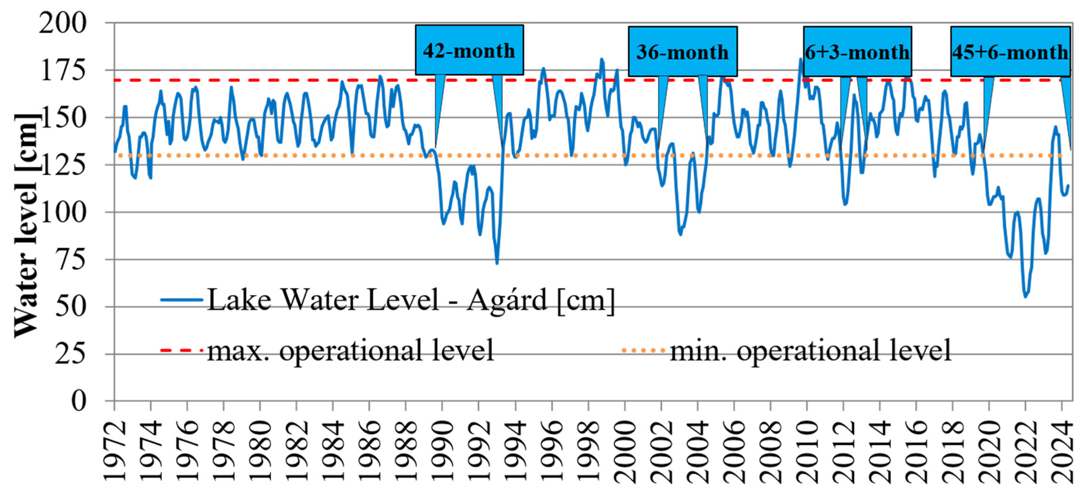
The lake exhibits strong spatial and functional heterogeneity. Reed beds largely cover the western part and serve as a protected ecological area, whereas the eastern part consists of open water and provides an intensively used recreational area. As a result, two upstream reservoirs and a controlled outflow tightly regulate water levels in Lake Velence. (See the water level time series in Figure 2.)

The two upstream reservoirs (Zámoly and Pátka), constructed in the 1970s, were originally designed to support water replenishment during dry periods by storing water during wetter seasons (November–April). Over time, their role has expanded beyond water regulation to include fisheries and recreational uses, which have contributed to increased nutrient loading. Combined with external inputs from agriculture and wastewater, this has led to eutrophication problems, occasionally limiting the usability of stored water for lake replenishment. In certain years, the reservoirs’ interception of streamflow has reduced direct runoff to the lake, effectively disconnecting a significant portion of the catchment.

Recent hydrological extremes have further highlighted the system’s vulnerability. Following a prolonged drought from 2020 to 2022, lake water levels reached a historical low of 53 cm in September 2022. This event triggered increased management pressure and a range of interventions, including partial wetland drainage and modifications to reservoir operation.

The Zámoly reservoir was emptied in 2021, while water from the Pátka reservoir was diverted towards the lake during the wet winter of 2023–2024. As of 2026, both reservoirs operate primarily as empty storage areas with limited and temporary active retention.

3.3. Data Sources

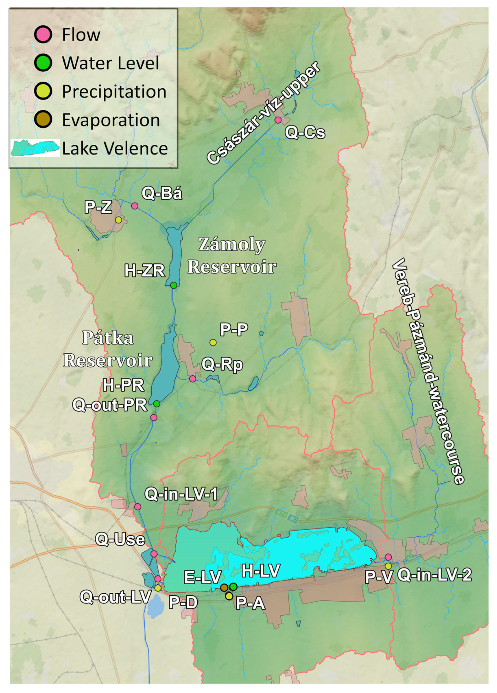
The Central Transdanubian Water Directorate (KDTVIZIG) provided the hydrometeorological and hydrographic data shown in

Table 1. Hydrometeorological data in the catchment of Lake Velence (source: KDTVIZIG).

Location	Symbols	Parameter	Frequency	Timeframe
Water level and bathymetric curves
Zámolyi reservoir	HZR (Obs) AZR = f(HZR) VZR = f(HZR)	H = Water level (cm) Observed A = Water surface (m2) as a function of H V = Water volume (m3) as a function of H	Monthly	1998–2024
Pátkai reservoir	HPR (Obs) APR = f(HPR) VPR = f(HPR)
Lake Velence	HLV (Obs) ALV = f(HLV) VLV = f(HLV)
Streamflow
Császár-víz (upper)—Csákvár	QCs	Q = Discharge (m3/s) Qin-LV = Qin-LV-1 + Qin-LV-2	Daily, Monthly	1998–2024
Burján-árok—Zámoly	QBá
Rovákja-patak—Pátka	QRp
Császár-víz—Kisfalud	Qin-LV-1
Vereb-Pázmánd watercourse—Kápolnásnyék	Qin-LV-2
Zámolyi Reservoir outflow	Qout-ZR		Monthly
Pátkai Reservoir outflow	Qout-PR
DIT (nursery pond) water abstraction	QUse
Lake Velence outflow structure—Dinnyés	Qout-LV
Precipitation
Zámoly	PZ	P = Rainfall (mm)	Monthly	1998–2024
Pátka	PP
Dinnyés	PD	Average rainfall: ${\mathrm{P}}_{\mathrm{L}\mathrm{V}}={\displaystyle \frac{{\mathrm{P}}_{\mathrm{D}}+{\mathrm{P}}_{\mathrm{A}}+{\mathrm{P}}_{\mathrm{V}}}{3}}$ (mm)	Daily, Monthly
Agárd	PA
Velence	PV
Agárd	ELV	Actual lake evaporation (mm)—calculated	Monthly	1998–2024

and Figure 3. The dataset covers the period 1998–2024 and includes water levels, bathymetric relationships, streamflow, precipitation, and evaporation. The dataset integrates measurements from multiple components of the system, including the two reservoirs, the lake, and their tributaries and outflows. Bathymetric curves complement water level observations by describing the relationships among water level, surface area, and storage volume for each water body.

Streamflow data include measured inflows, reservoir releases, and outflows from the lake system. Multiple stations within the catchment record precipitation, and lake-wide precipitation is calculated as a spatial average. Evaporation data are derived from measurements at the Agárd station. All variables were processed to ensure consistency in subsequent modeling. Streamflow values (m³/s) were converted to monthly volumes, while precipitation and evaporation (mm) were transformed into volumetric units using the corresponding water surface areas.

4. Water Balance Calculations

4.1. Current Water Balance Calculation Method

The Water Directorate has calculated the monthly water balance of Lake Velence since 1986 using the following equation:

P_LV + Q_in-LV + Q_out-PR + Z_month = E_LV + Q_out-LV + Q_Use ± ∆H_LV

where

P_LV is the monthly precipitation falling on Lake Velence (lake-mm);

Q_in-LV is the total monthly inflow from tributaries with multipliers to account for unmeasured inflow;

Q_out-PR represents releases from the upstream reservoir system;

Z_month is the residual error term calculated by subtracting the observed water level from the calculated water level;

E_LV is lake evaporation;

Q_out-LV is the outflow from the lake;

Q_Use is water abstraction;

ΔH_LV is the observed change in lake water level.

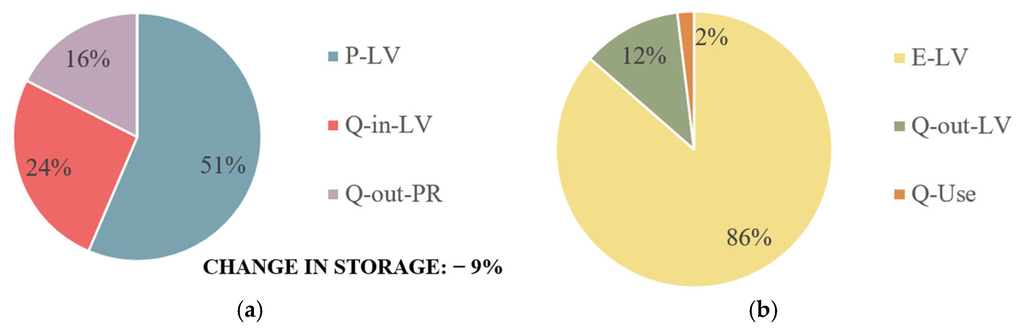
Figure 4 presents the contribution of water budget inflow and outflow elements to the water balance of Lake Velence between 1998 and 2024 according to the current calculation method.

Note that reservoir releases are treated separately from natural inflows, and upstream reservoir dynamics are not explicitly integrated into the balance. Since the water balances for the two upstream reservoirs are not systematically calculated, the current method does not fully capture the mass balance of the coupled reservoir–lake system.

Monthly residual errors (Z) of the current water balance calculation result from subtracting observed water levels from the calculated water levels. In practice, residual errors are redistributed retrospectively at the end of each year among selected components (precipitation, evaporation, and inflow) based on expert judgment to achieve annual closure. While this ensures formal closure, it does not resolve underlying systematic errors.

Previous analyses have shown that, before error redistribution, the average annual water balance error was approximately −70 lake-mm/year for the 1986–2022 period [35]. A negative error indicates that the calculated lake water level is lower than the observed water level. The magnitude of this error is comparable to the average annual variation in the lake water level. Furthermore, it corresponds to approximately 13% of the mean annual precipitation. These results indicate the presence of significant systematic errors or potentially missing components in the water balance equation.

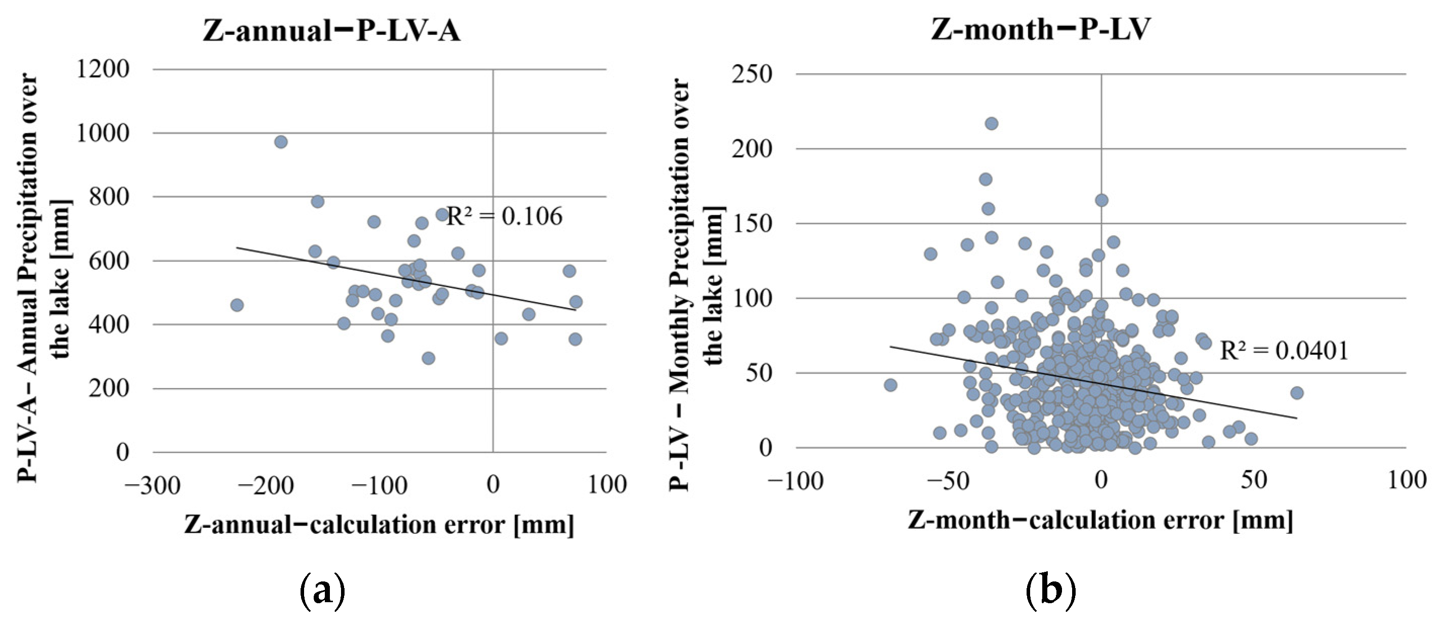
Further analysis of error characteristics revealed relationships between water balance components and residual errors [35,36]. A weak negative correlation was identified between precipitation and the error term, indicating that the water balance tends to underestimate lake water levels during wetter periods and overestimate them during drier conditions. Figure 5 illustrates the relationship between precipitation and water balance error.

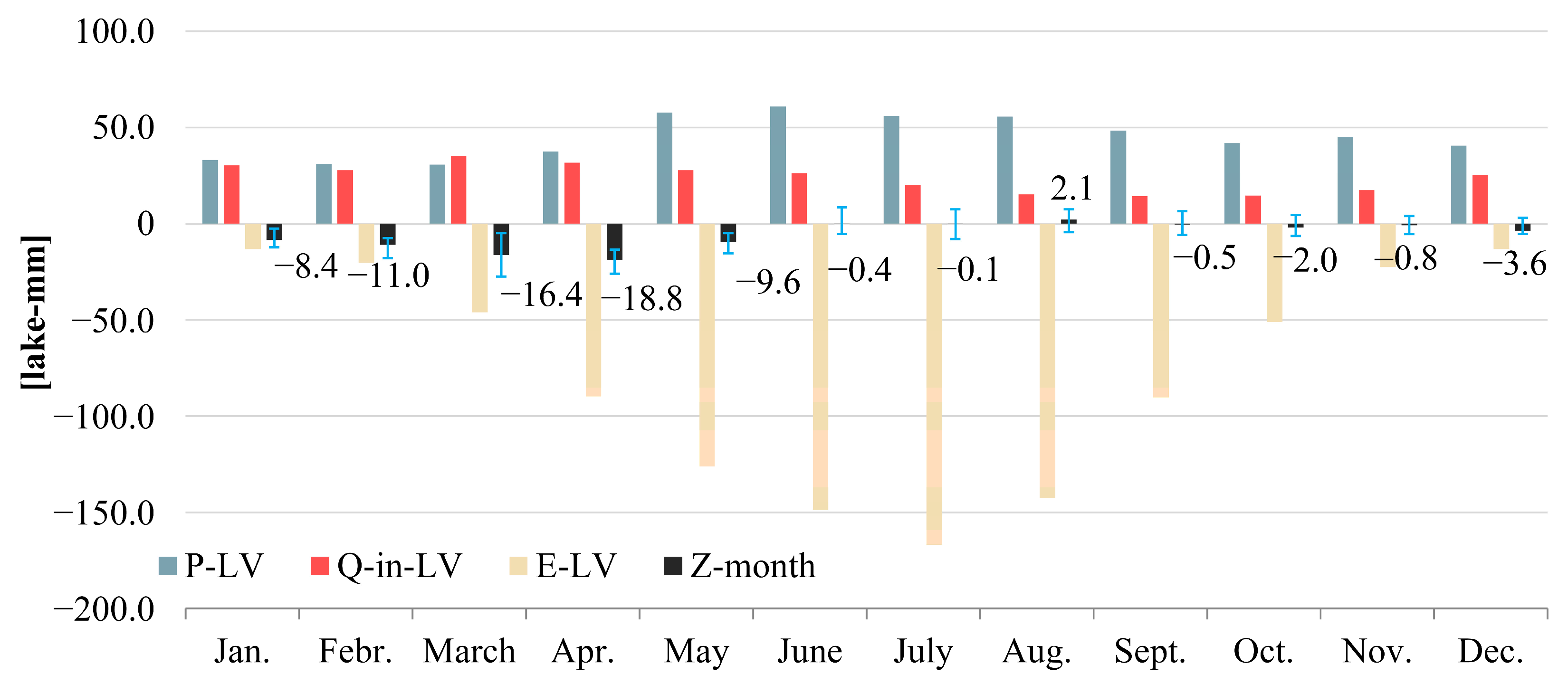
This finding initially suggested systematic underestimation of precipitation measurements. However, a more detailed analysis of the temporal structure of the errors provided additional insight. Average monthly errors were close to zero during the June–November period, while consistently negative values occurred between December and May, with a peak of −18.8 lake-mm/month in April [36]. Figure 6 shows the monthly components of water balance and errors.

This pronounced seasonal pattern contradicts the assumption of purely random errors and indicates the presence of systematic, time-dependent biases or missing processes affecting the winter–spring period. The temporal structure of the errors suggests that precipitation bias alone cannot fully explain the observed discrepancies.

As an alternative explanation, recent studies have investigated the role of groundwater exchange. Baják et al. [37] applied a three-dimensional transient groundwater flow model to estimate subsurface inflows and outflows, suggesting a net groundwater inflow of approximately 47 lake-mm/year. Incorporating this component would substantially reduce the observed annual deficit, although the temporal distribution has not yet been compared to residual errors. The current water balance calculation method exhibits significant uncertainty, reliance on retrospective adjustments, and a lack of consistent representation of the full reservoir–lake system. Therefore, the raw time series of measured and calculated components are not directly suitable for continuous modeling or for evaluating water management scenarios.

These limitations motivated the development of a revised methodology capable of closing the joint water balance of the cascaded system.

4.2. Methodological Framework

The proposed methodology aims to calculate and close the joint, continuous water balance of a cascaded system comprising two upstream reservoirs and a downstream lake at a monthly time step over multiple decades.

The workflow consists of five sequential stages:

• Baseline modeling (Model-A): Construction of a continuous water balance using raw measured data without bias correction.
• Bias correction (Model-B): Application of a linear correction framework with uniform coefficients to reduce systematic errors.
• Seasonal correction (Model-C): Extension of Model-B by introducing seasonally varying coefficients based on observed error patterns.
• Residual diagnostics: Evaluation of model assumptions and identification of remaining biases.
• Validation and performance assessment: Comparison of model performance over an independent validation period.

All models operate on a monthly time step, and storage is updated sequentially along the cascade.

4.3. Model-A: Baseline Water Balance Model

4.3.1. System Equations

Model-A represents the joint water balance of the cascaded reservoir–lake system using measured input data. The system represents a continuous mass balance model with a monthly time step, in which storage in each water body is updated sequentially along the cascade (from the upstream reservoir to the downstream lake) based on inflows and outflows. For each month i, the change in storage (ΔV) is calculated from all inflow and outflow components, and total storage is updated cumulatively from the initial observed state. Water levels at the beginning of each time step are then derived from storage using bathymetric relationships.

Figure 7 illustrates the conceptual structure of the cascade system.

The calculation process uses two different indices. Index k represents the month of interest, while index i represents a general month in the summation. The remaining terms in the following equations are presented in Table 1 and Figure 7b.

The calculated water level of Zámoly Reservoir at the beginning of month k uses its bathymetric curves:

$${H_{\mathit{Z}R}\left(C\right)}_k=f\left({V_{\mathit{Z}R}\left(C\right)}_k\right)$$

(1)

The calculated volume of Zámoly Reservoir at the beginning of month k is:

$${V_{\mathit{Z}R}\left(C\right)}_k=\max \left\{\begin{array}{c}{V}_{\mathit{Z}R}{\left(Obs\right)}_0+{\sum }_{i=0}^{k-1}{{∆V}_{\mathit{Z}R}\left(C\right)}_i\\ 0\end{array}\right\}$$

(2)

where $V_{\mathit{Z}R}{\left(Obs\right)}_0$ is the initial observed water level of the Zámoly reservoir on 1/1/1998.

The calculated change in volume for Zámoly Reservoir in month i is (see conceptual model, Figure 7b, and Table 1):

$${{∆V}_{\mathit{Z}R}\left(C\right)}_i^{Model-A}=V\left(P_{\mathit{Z},i}\right)+V\left(Q_{B\mathrm{á},i}\right)+V\left(Q_{Cs,i}\right)-{V(E}_{\mathit{Z},i})-\left\{V\left(Q_{out-\mathit{Z}R,i}\right)\right\}$$

(3)

where V denotes volume calculated from measured discharge, precipitation, or evaporation data. The final term in {} connects the cascade between Zámoly and Pátka Reservoirs.

The calculated water level of Pátka Reservoir using its bathymetric curves, at the beginning of month k, is:

$${H_{\mathit{P}R}\left(C\right)}_k=f\left({V_{\mathit{P}R}\left(C\right)}_k\right)$$

(4)

The calculated volume of Pátka Reservoir at the beginning of month k is:

$${V_{\mathit{P}R}\left(C\right)}_k=\max \left\{\begin{array}{c}{V}_{\mathit{P}R}{\left(Obs\right)}_0+{\sum }_{i=0}^{k-1}{{∆V}_{\mathit{P}R}\left(C\right)}_i\\ 0\end{array}\right\}$$

(5)

where $V_{\mathit{P}R}{\left(Obs\right)}_0$ is the initial observed water level of Pátka Reservoir on 1/1/1998.

The calculated change in volume for Pátka Reservoir in the i-th month is:

$${{∆V}_{\mathit{P}R}\left(C\right)}_i^{Model-A}=V\left(P_{\mathit{P},i}\right)+V\left(Q_{Rp,i}\right)+\left\{V\left(Q_{out-\mathit{Z}R,i}\right)\right\}-{V(E}_{\mathit{P},i})-⟦V\left(Q_{out-\mathit{Z}R,i}\right)⟧$$

(6)

where V denotes volume calculated from measured discharge, precipitation, or evaporation data. The {} term from Equation (3) is now an input, and the ⟦ ⟧ term cascades to Lake Velence.

The calculated water level of Lake Velence using its bathymetric curves, at the beginning of the k-th month, is:

$${H_{\mathit{L}\mathit{V}}\left(C\right)}_k=f\left({V_{\mathit{L}\mathit{V}}\left(C\right)}_k\right)$$

(7)

The calculated volume of Lake Velence at the beginning of month k is:

$${V_{\mathit{L}\mathit{V}}\left(C\right)}_k=V_{\mathit{L}\mathit{V}}{\left(Obs\right)}_0+{\displaystyle \sum _{i=0}^{k-1}}{{∆V}_{\mathit{L}\mathit{V}}\left(C\right)}_i$$

(8)

where $V_{\mathit{L}\mathit{V}}{\left(Obs\right)}_0$ is the initial observed water level of Lake Velence on 1/1/1998.

The calculated change in volume for Lake Velence in month i is:

$$\begin{gathered} {{∆V}_{\mathit{L}V}\left(C\right)}_i^{Model-A}=V\left(P_{\mathit{L}\mathit{V},i}\right)+V\left(Q_{in \mathit{L}\mathit{V},i}\right)+⟦V\left(Q_{out-\mathit{P}R,i}\right)⟧-V\left(E_{\mathit{L}\mathit{V},i}\right) \\ -V\left(Q_{out-\mathit{L}\mathit{V},i}\right)-V\left(Q_{use,i}\right) \end{gathered}$$

(9)

where the ⟦ ⟧ term from Equation (6) connects Pátka Reservoir to Lake Velence.

4.3.2. System Coupling (Joint Water Balance)

The water balance model is formulated as a joint system, in which the three water bodies are hydraulically connected. Outflows from the upstream Zámoly Reservoir, V(Q_{out-ZR, i}), are treated as inflows to the downstream Pátka Reservoir (Equations (3) and (6)). Similarly, releases from Pátka Reservoir, V(Q_{out−PR, i}), are considered as inflows to Lake Velence (Equations (6) and (9)). The two creeks connecting the three water bodies have negligible volumes compared to the reservoirs and the lake. Their travel times are short when viewed on a monthly basis. This configuration ensures that mass is conserved across the entire cascade and that interactions between upstream and downstream components are explicitly represented.

4.3.3. Time Step and Unit Conversion (Monthly Resolution)

The model operates on a monthly time step, with all fluxes aggregated over each month $i$. Streamflow variables measured in m³/s (e.g., $Q_{out-ZR,i}$) are converted to monthly volumes $V\left(Q_{out-ZR,i}\right)$ by multiplying by the number of seconds in the respective month.

Precipitation volumes (e.g., $V\left(P_{Z,i}\right)$) are calculated by multiplying monthly precipitation depth (mm) by the water surface area of the respective water body at month $i$. Similarly, evaporation volumes are calculated using the evaporation depth calculated from measured data at the Agárd station and the surface area of each reservoir or lake.

All variables are consistently converted to volumetric units (m³) to ensure compatibility within the mass balance framework. In larger systems, time lags between connected water bodies may need to be considered. However, no time lag was introduced in this study, as the water travel time within the system is on the order of days, which is negligible compared to the monthly modeling time step.

4.3.4. Continuous Storage Calculation and Residuals

The model is formulated as a continuous storage system, in which water volumes are updated cumulatively over time. For each water body, total storage at the beginning of month $k$ is calculated by summing all monthly storage changes from the initial observed volume up to month $k-1$ (Equations (2), (5) and (8)). Water levels are then derived from storage using bathymetric relationships (Equations (1), (4) and (7)). Model residuals are calculated as:

$${H_{\mathit{Z}R}\left(Obs\right)}_k={H_{\mathit{Z}R}\left(C\right)}_k-{\epsilon }_{\mathit{Z}R, k}\to {\epsilon }_{\mathit{Z}R, k}={H_{\mathit{Z}R}\left(C\right)}_k-{H_{\mathit{Z}R}\left(Obs\right)}_k$$

(10)

$${H_{\mathit{P}R}\left(Obs\right)}_k={H_{\mathit{P}R}\left(C\right)}_k-{\epsilon }_{\mathit{P}R, k}\to {\epsilon }_{\mathit{P}R, k}={H_{\mathit{P}R}\left(C\right)}_k-{H_{\mathit{P}R}\left(Obs\right)}_k$$

(11)

$${H_{\mathit{L}\mathit{V}}\left(Obs\right)}_k={H_{\mathit{L}\mathit{V}}\left(C\right)}_k-{\epsilon }_{\mathit{L}\mathit{V}, k}\to {\epsilon }_{\mathit{L}\mathit{V}, k}={H_{\mathit{L}\mathit{V}}\left(C\right)}_k-{H_{\mathit{L}\mathit{V}}\left(Obs\right)}_k$$

(12)

Since water levels are derived from cumulative storage, these residuals represent the cumulative effect of errors in all water balance components up to the k-th time step.

4.3.5. Representation of Reservoir Operation

Reservoir operation is explicitly incorporated to reproduce observed emptying conditions. When, according to observations, the reservoir contains water at the end of a time step, the measured outflow is applied. When the reservoir is empty, outflow is constrained to prevent simulated storage from exceeding the physically available water. The outflow is therefore limited by the maximum of the following amounts: (1) measured outflow, (2) available inflow plus precipitation minus evaporation, and (3) initial storage at the beginning of the time step. This formulation enforces consistency between observed and simulated reservoir states while preserving mass balance.

4.4. Model-B: Linear Bias Correction Model with Uniform Coefficients

The results from the baseline water balance model (Model-A) indicate significant systematic bias when using raw measured data, preventing reliable long-term simulations. (See Section 5.) Therefore, new models that carry out bias correction are introduced. In a first attempt, Model-B applies multiple linear regression (MLR) bias correction, in which coefficients are used to adjust water balance components. In Model-B, these coefficients are assumed to be constant over time and are applied uniformly across all months.

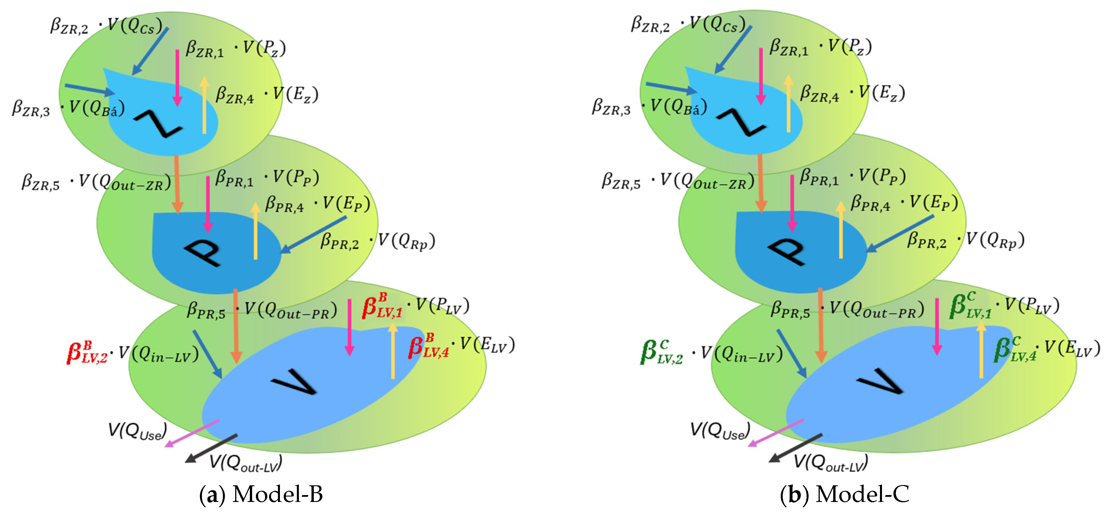
Equations (13)–(15) define the corrected storage change $(\Delta V_i)$ equations for Zámoly Reservoir, Pátka Reservoir, and Lake Velence, respectively. These equations replace the corresponding mass balance equations of Model-A (Equations (3), (6) and (9)) while preserving the original structure of inflow and outflow components. Figure 8 presents conceptual figures of the MLR models.

$$\begin{gathered} {{∆V}_{\mathit{Z}R}\left(C\right)}_i^{Model-B,C}={\beta }_{ZR,0}+{\beta }_{ZR,1} V\left(P_{\mathit{Z},i}\right)+{\beta }_{ZR,2} V\left(Q_{Cs,i}\right)+ \\ {\beta }_{ZR,3} V\left(Q_{B\mathrm{á},i}\right)-{\beta }_{ZR,4} {V(E}_{\mathit{Z},i})-{\beta }_{ZR,5} \left\{V\left(Q_{out-\mathit{Z}R,i}\right)\right\} \end{gathered}$$

(13)

$$\begin{gathered} {{∆V}_{\mathit{P}R}\left(C\right)}_i^{Model-B,C}={\beta }_{PR,0}+{\beta }_{PR,1} V\left(P_{\mathit{P},i}\right)+{\beta }_{PR,2} V\left(Q_{Rp,i}\right)+ \\ {\beta }_{PR,3} \left\{V\left(Q_{out-\mathit{Z}R,i}\right)\right\}-{\beta }_{PR,4} {V(E}_{\mathit{P},i})-{\beta }_{PR,5}⟦V\left(Q_{out-\mathit{P}R,i}\right)⟧ \end{gathered}$$

(14)

$$\begin{gathered} {{∆V}_{\mathit{L}\mathit{V}}\left(C\right)}_i^{Model-B}={\beta }_{LV,0}^B+{\beta }_{LV,1}^B V\left(P_{\mathit{L}\mathit{V},i}\right)+{\beta }_{LV,2}^{B}V\left(Q_{in,i}\right)+{\beta }_{LV,3}^B⟦V\left(Q_{out-\mathit{P}R,i}\right)⟧ \\ -{\beta }_{LV,4}^{B}V\left(E_{\mathit{L}\mathit{V},i}\right)-{\beta }_{LV,5}^{B,C} V\left(Q_{out-\mathit{L}\mathit{V},i}\right)-{\beta }_{LV,6}^{B,C}V\left(Q_{use,i}\right) \end{gathered}$$

(15)

In the equations, the subscripts of the $\beta$ regression coefficients denote the associated water body (ZR: Zámoly Reservoir, PR: Pátka Reservoir, LV: Lake Velence), and balance components: 1 represents precipitation, 2 and 3 represent inflow, 4 represents evaporation, and 5 represents outflow from the respective water body.

4.4.1. Parameter Selection and Model Structure

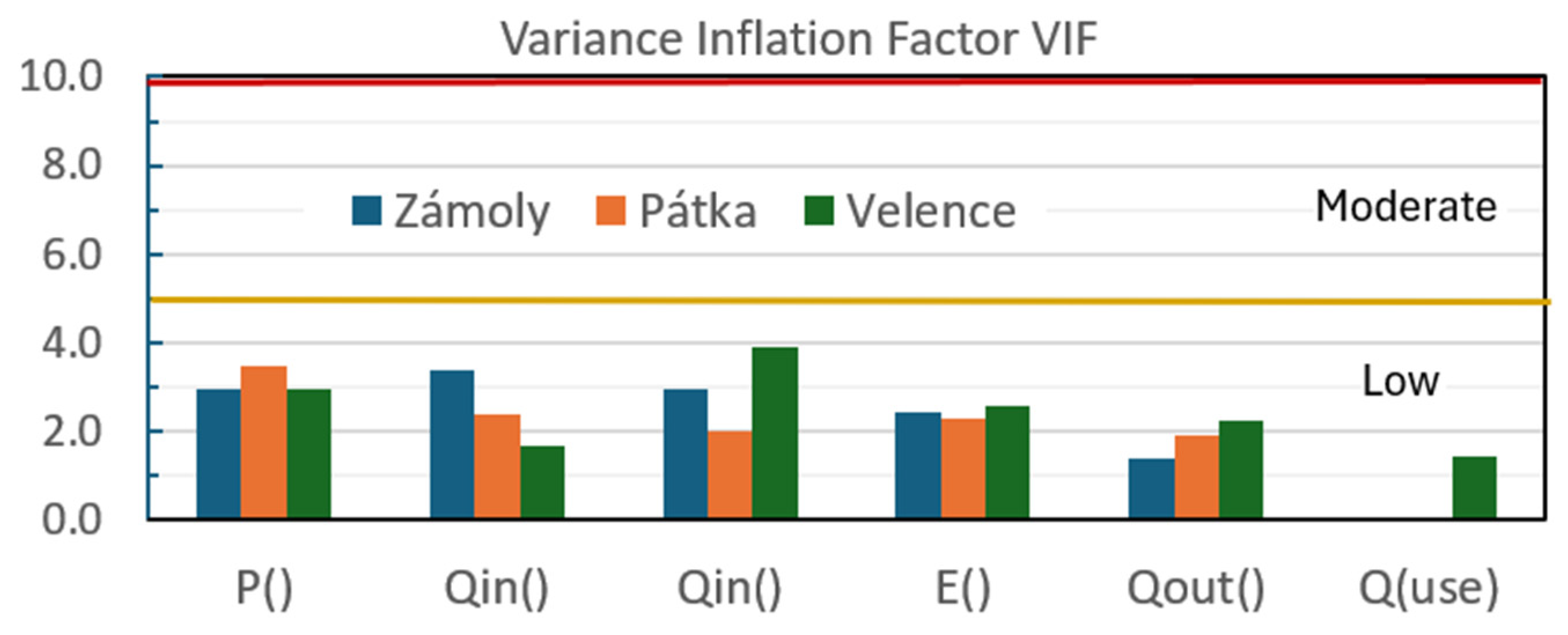
Preliminary statistical analysis identified precipitation, inflow, and evaporation as significant predictors based on Student’s t-tests. Furthermore, pairwise correlation analysis and Variance Inflation Factors (VIFs) were evaluated to verify that multicollinearity among the candidate predictors remained sufficiently low for reliable coefficient estimation [38]. As a result, the corresponding coefficients (β_ZR,1, β_ZR,2, β_ZR,3; β_ZR,4; β_PR,1, β_PR,2, β_PR,4; β_LV,1, β_LV,2, β_LV,4) were included in the calibration. In addition, coefficients for reservoir outflow (β_ZR,5 = β_PR,3; and β_PR,5 = β^B,C_LV,3) were calibrated to approximate overall mass balance across the cascade. MLR coefficients of the remaining components (β^B,C_LV,5, β^B,C_LV,6) were fixed at 1, while the intercepts (constant terms), β_ZR,0, β_PR,0, and β_LV,0, were considered 0. Retaining only statistically significant predictors and verifying low multicollinearity improves parameter identifiability and reduces the likelihood of unstable coefficient estimates [38].

4.4.2. Calibration Procedure

Coefficients were estimated sequentially for each water body, starting from Zámoly Reservoir (upstream), followed by Pátka Reservoir (intermediate), and ending with Lake Velence (downstream). This sequential calibration ensured that corrected outflows from upstream components correctly propagated as inflows to downstream elements. Calibration sought to minimize the root-mean-square error (RMSE) between simulated and observed water levels. RMSE was selected because it quantifies prediction error in the physical units of the state variable (cm) and gives greater weight to larger deviations [39], which are particularly important in long-term water balance simulations where cumulative volume errors propagate through time.

Although the regression coefficients are included linearly in the water balance equations, the calibration problem itself is nonlinear. This is because simulated storage is updated recursively, so each month’s prediction depends on the corrected storage changes from all previous months. Consequently, parameter estimation was performed using the Generalized Reduced Gradient (GRG) nonlinear optimization algorithm [40], implemented in Microsoft Excel [41]. To reduce the risk of convergence to local minima, a multi-start procedure was applied, with a population size of 100 and a fixed random seed value of 10 for each water body. Coefficient bounds (see

Table 2. Boundaries of MLR coefficients used when calibrating Model-B and Model-C.

MLR Coefficient	Lower Boundary	Upper Boundary
βZR,1, βZR,2, βZR,3, βZR,5	0.60	2.00
βZR,4, βPR,4, βPR,5	0.70	1.50
βPR,1, βPR,2, βLV,1, βLV,2, βLV,4	0.75	1.30

) were defined to reflect physical plausibility and constrain the solution space, accounting for expected uncertainties across different water balance components.

The imposed limits prevented the use of physically unrealistic correction factors while allowing sufficient flexibility to compensate for systematic bias. As shown in Table 2, coefficients β_ZR,1, β_ZR,2, β_ZR,3, and β_ZR,5 (related to Zámoly Reservoir) were allowed wider bounds to account for the greater uncertainty in this reservoir’s water balance. This uncertainty is likely caused by unmeasured surface inflows entering Zámoly Reservoir between the Csákvár discharge gauging station and the reservoir itself (see Figure 2), resulting in an apparent imbalance between the measured inflows and the recorded reservoir releases.

4.5. Model-C: Seasonal Bias Correction Model

Previous studies, as summarized in Section 4.1, have shown that long-term average monthly water balance errors of Lake Velence exhibit a clear seasonal pattern, with significant negative errors during the December–May period and values close to zero during June–November [36]. Based on this observation, the underlying hypothesis of Model-C is that systematic errors are temporally structured and primarily affect the winter–spring period. Therefore, in Model-C, bias correction is applied selectively only during these months, while unmodified measured water balance components are used during June–November. The formulation for Lake Velence is given in Equation (16), replacing Equation (15) of Model-B.

$${{∆V}_{\mathit{L}\mathit{V}}\left(C\right)}_i^{Model-C}=\mathrm{if}\left\{\begin{array}{c}(Dec.-May) {\beta }_{LV,0}^C+{\beta }_{LV,1}^C V\left(P_{\mathit{L}\mathit{V},i}\right)+{\beta }_{LV,2}^C V\left(Q_{in,i}\right)+{\beta }_{LV,3}^{C}V\left(Q_{out-\mathit{P}R,i}\right) \\ -{\beta }_{LV,4}^C{V(E}_{\mathit{L}\mathit{V},i})-{\beta }_{LV,5}^{B,C} V\left(Q_{out-\mathit{L}\mathit{V},i}\right)- {\beta }_{LV,6}^{B,C} V\left(Q_{Use,i}\right) \\ L\\ (June-Nov.) V\left(P_{\mathit{L}\mathit{V},i}\right)+V\left(Q_{in,i}\right)+V\left(Q_{out-\mathit{P}R,i}\right)-{V(E}_{\mathit{L}\mathit{V},i}) \\ -V\left(Q_{out-\mathit{L}\mathit{V},i}\right)-V\left(Q_{use,i}\right) \\ \end{array}\right\}$$

(16)

In this formulation, MLR coefficients for Lake Velence (β_LV,x) are applied only during the period with identified systematic bias, while the original mass balance formulation of Model-A is retained during months with negligible average error. The subscripts of the regression coefficients are associated with the same water balance components as in Model-B.

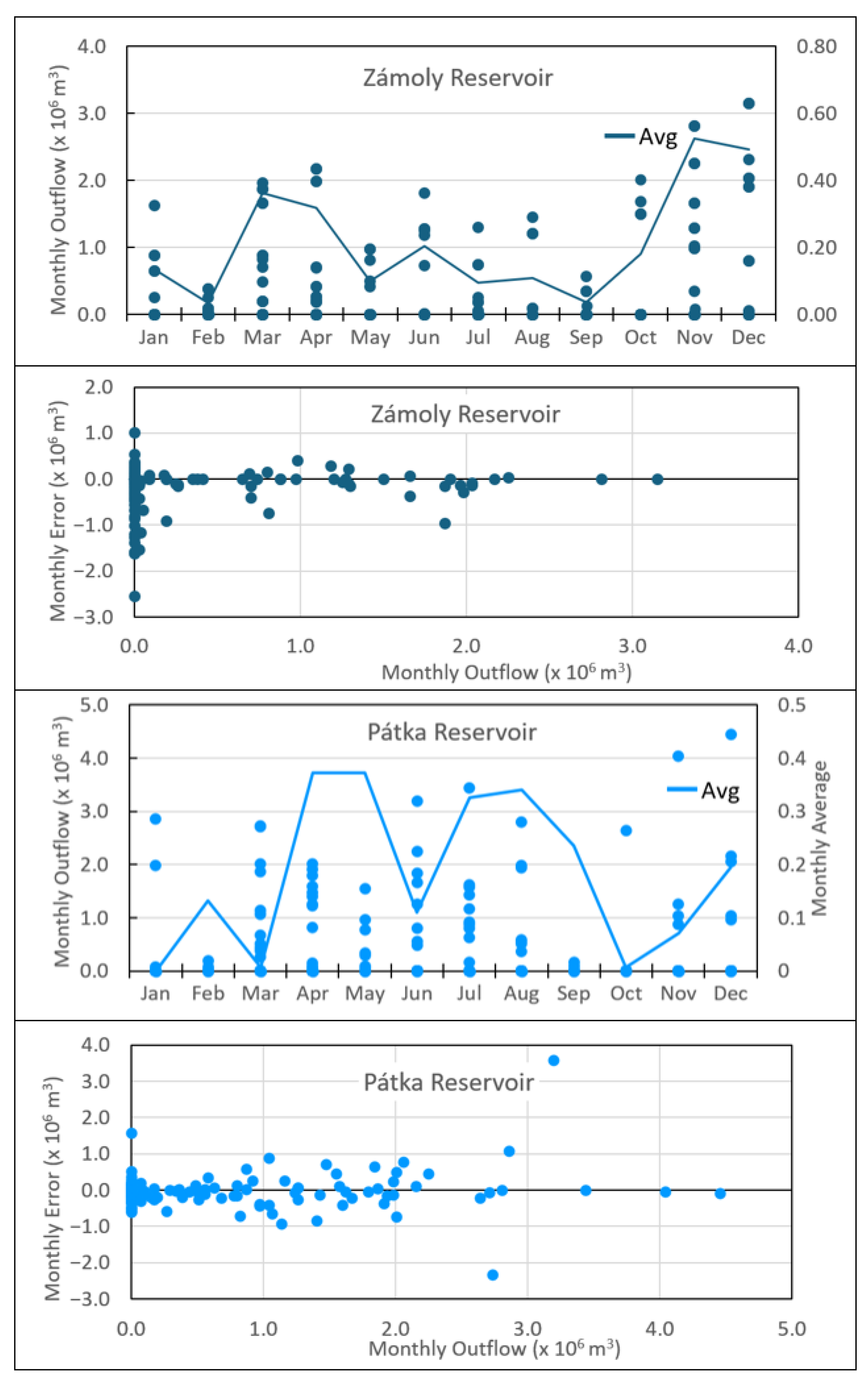
A review of the data comparing release volumes from the reservoirs to errors concerning their volume estimates found no discernible pattern, seasonal or otherwise. Figure 9 shows outflow volumes and Model-A residuals for the Zámoly and Pátka reservoirs from 1998 to 2017. During this time, zero outflow occurred in 189 of the 240 months for Zámoly and in 168 for Pátka. The figure illustrates the absence of seasonal cycles, particularly given that the majority of outflow volumes were zero. The residuals from Model-A show a random distribution with the magnitude of outflow volume as well. Therefore, the analysis did not consider seasonal adjustment factors for either reservoir. This decision was further reinforced by the calibration and verification runs, which showed no cyclic behavior in the residuals from these two reservoirs. The seasonal correction approach was applied only to Lake Velence. For the Zámoly and Pátka reservoirs, monthly storage changes were calculated using Model-B (Equations (13) and (14)), and the resulting corrected outflows were used as inputs for Lake Velence. This hybrid approach allowed the model to incorporate observed seasonal error patterns while maintaining consistency in the upstream components of the cascade.

4.6. Residual Diagnostics and Model Assumptions

Model performance was further evaluated through residual diagnostics. The criteria were assessed by (1) multicollinearity of input variables (Variance Inflation Factor), (2) autocorrelation of residuals (e.g., autocorrelation function), (3) normality of residuals (distribution analysis), and (4) homoscedasticity (variance consistency).

These diagnostics were used to evaluate the validity of regression assumptions and to identify remaining model deficiencies. Schmidt and Finan [33] point out that, for large sample sizes, violating the normality assumption does not markedly affect the results, and the focus should be on the independence and low multicollinearity of the inputs, as well as the homoscedasticity of the residual errors.

4.7. Validation and Performance Assessment

The models were calibrated for the period 1998–2017. The stability of the calibrated coefficients was assessed by applying the calibrated parameter sets without modification during the independent validation period (2018–2024), thereby evaluating their transferability beyond the calibration dataset. For both the calibration and validation periods, model performance was evaluated using Nash–Sutcliffe Efficiency (NSE) [42].

5. Results

5.1. Performance of the Baseline Model (Model-A)

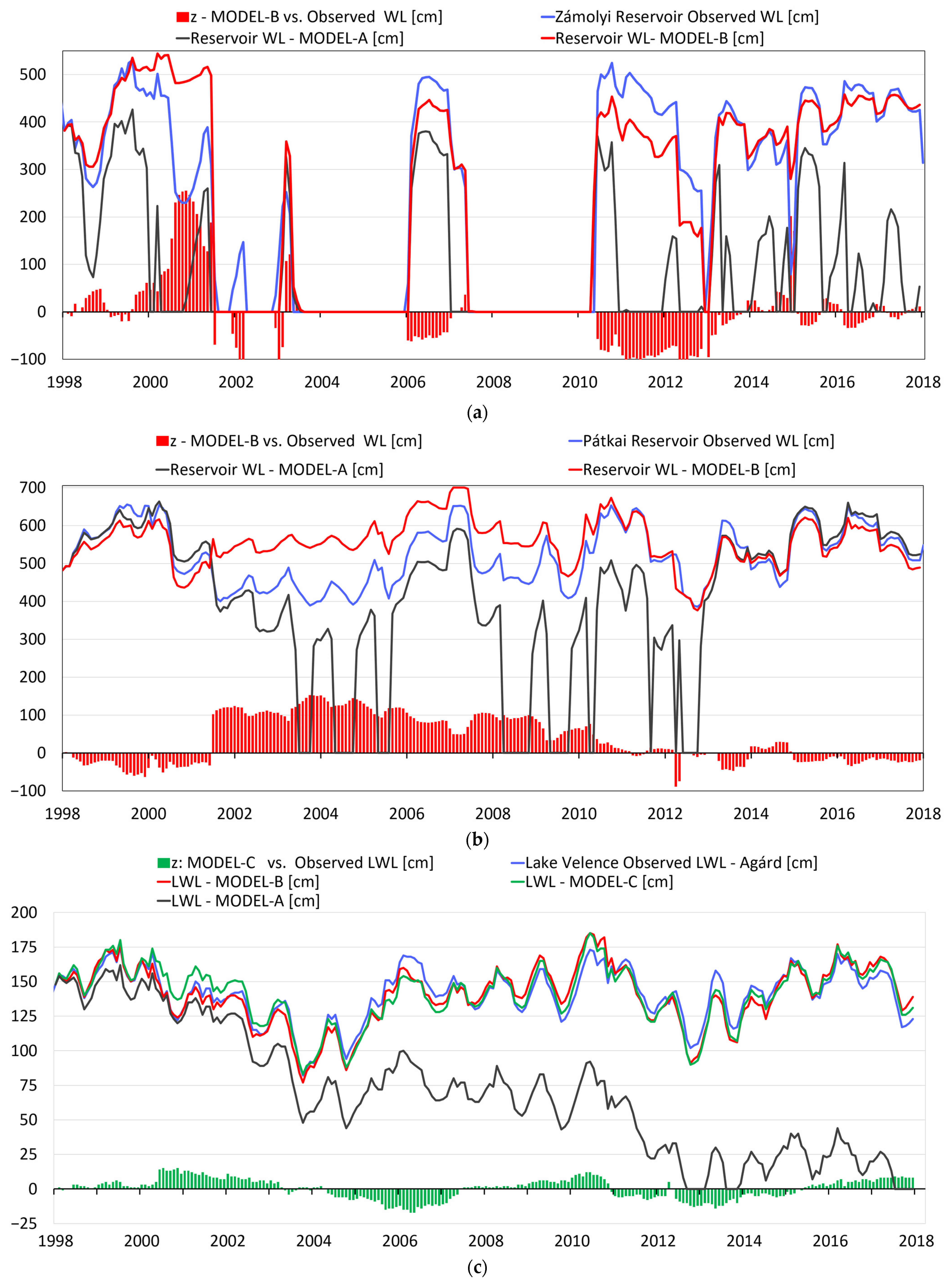
The water levels of Zámoly Reservoir, Pátka Reservoir, and Lake Velence were first simulated using the baseline water balance formulation (Model-A), based solely on measured and calculated but uncorrected input data, as shown in Figure 10a–c with a black line. The results show that Model-A produces rapidly diverging and physically unrealistic water levels within a few years. The accumulation of systematic errors in the water balance components propagates through the continuous storage calculation. The performance of Model-A for Zámoly Reservoir is NSE-A_ZR = −0.28; for Pátka Reservoir, NSE-A_PR = −5.13; and for Lake Velence, NSE-A_LV = −18.69. As a result, Model-A is unsuitable for long-term simulation of the cascaded system.

The divergence is observed consistently across all three water bodies, indicating that errors are systematic and propagate through the interconnected cascade. Since storage is computed continuously, even small biases in individual components accumulate over time, leading to large deviations in simulated water levels. The accumulation confirms the violation of the zero-mean residuals assumption, so the current measurement-based water balance cannot be used for long-term simulation without correction. Importantly, the divergence is observed consistently across all three water bodies, indicating that the issue is not localized but affects the entire cascaded system. This observation supports the hypothesis that errors propagate both temporally and spatially within interconnected systems.

5.2. Input Variable Analysis and Model Setup

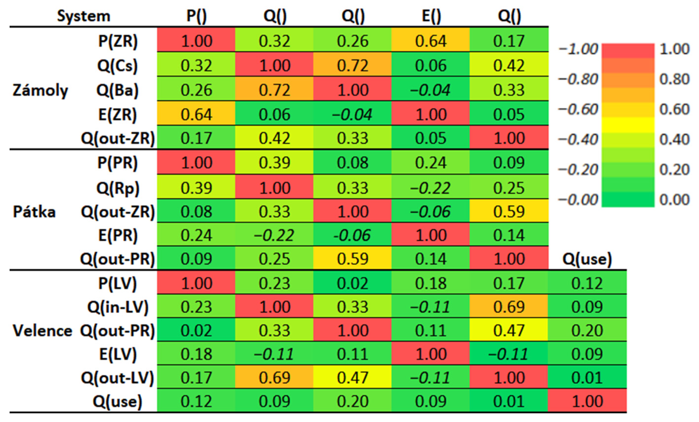
Before applying the two MLR models, the statistical properties of the input variables were evaluated to ensure the validity of the modeling framework. Pairwise correlations and multicollinearity were assessed for each water body, as shown in Figure 11 and Figure 12.

Moderate correlations were observed between inflow and outflow variables, reflecting the physical connectivity of the cascade system. However, multicollinearity remained within acceptable limits, with all Variance Inflation Factors (VIFs) below 5. For Lake Velence, most variables were weakly correlated, except inflow (Q_in) and outflow (Q_out). Since Q_out is directly measured, while Q_in partly includes estimated components, Q_out was considered more reliable. In addition, based on statistical testing (Student-t), Q_in showed higher explanatory power; therefore, Q_out was excluded from the regression formulation.

5.3. Performance of the Bias-Corrected Model (Model-B)

Model-B (red curves in Figure 10a–c) results in a substantial improvement over Model-A. The simulated water levels show improved agreement with observations: Zámoly Reservoir: NSE = B_ZR = 0.89, Pátka Reservoir: NSE-B_PR = 0.17, and Lake Velence: NSE-B_LV = 0.83.

The relatively low NSE for the Pátka Reservoir resulted from known inconsistencies in the measured reservoir release data from Zámoly and Pátka Reservoirs in June 2001. The large absolute error caused by this one month persisted over several years, up until 2010. Meanwhile, the model approximated monthly changes in water storage well. Overall, Model-B significantly reduces systematic bias and stabilizes long-term simulations.

Table 3. Final MLR coefficients used when calibrating Model-B and Model-C.

MLR Coefficient	Zámoly Reservoir	Pátka Reservoir	Lake Velence
			Model-B	Model-C
Precipitation	βZR,1 = 1.040	βPR,1 = 1.300	βBLV,1 = 1.270	βCLV,1 = 1.260
Inflow-1	βZR,2 = 1.940	βPR,2 = 0.870	βBLV,2 = 0.815	βCLV,2 = 0.815
Inflow-2	βZR,3 = 1.200	βPR,3 = 0.700 1	βBLV,3 = 0.820 2	βCLV,3 = 0.820 2
Evaporation	βZR,4 = 0.914	βPR,4 = 1.130	βBLV,4 = 0.988	βCLV,4 = 0.970
Outflow	βZR,5 = 0.700 1	βPR,5 = 0.820 2	βBLV,5 = 1.000	βCLV,5 = 1.000

¹ Outflow from Zámoly = Inflow-2 to Pátka. ² Outflow from Pátka = Inflow-2 to Velence.

presents the calculated coefficients.

As discussed earlier, Table 3 shows that the upstream outflow coefficients equal the corresponding downstream inflow coefficients, ensuring consistency within the cascaded system. The forced agreement (two coefficients), setting the Velence to ground truth (one coefficient = 1.0), and forcing zero intercepts (three offset coefficients = 0.0) reduce the number of adjustable MLR coefficients from 18 to 12.

The improvement introduced by Model-B demonstrates that MLR bias correction of water balance components can effectively reduce systematic errors.

5.4. Performance of the Seasonal Model (Model-C)

For Lake Velence, Model-C (see green curve in Figure 10c) provides a moderate improvement over Model-B during the calibration period, with NSE increasing by 0.03 points from NSE-B_LV = 0.83 to NSE-C_LV = 0.86.

Although the increase in NSE is modest, the improvement introduced by Model-C is structurally important. By applying correction only during the December–May period, the model directly targets the time window where systematic errors are known to occur. This selective correction reduces seasonal bias without overfitting periods where the original data already perform well. As a result, Model-C provides a more balanced representation of the system, as shown later in the model performance assessment and final verification.

5.5. Model Performance Assessment

5.5.1. Model Accuracy and Structural Assessment

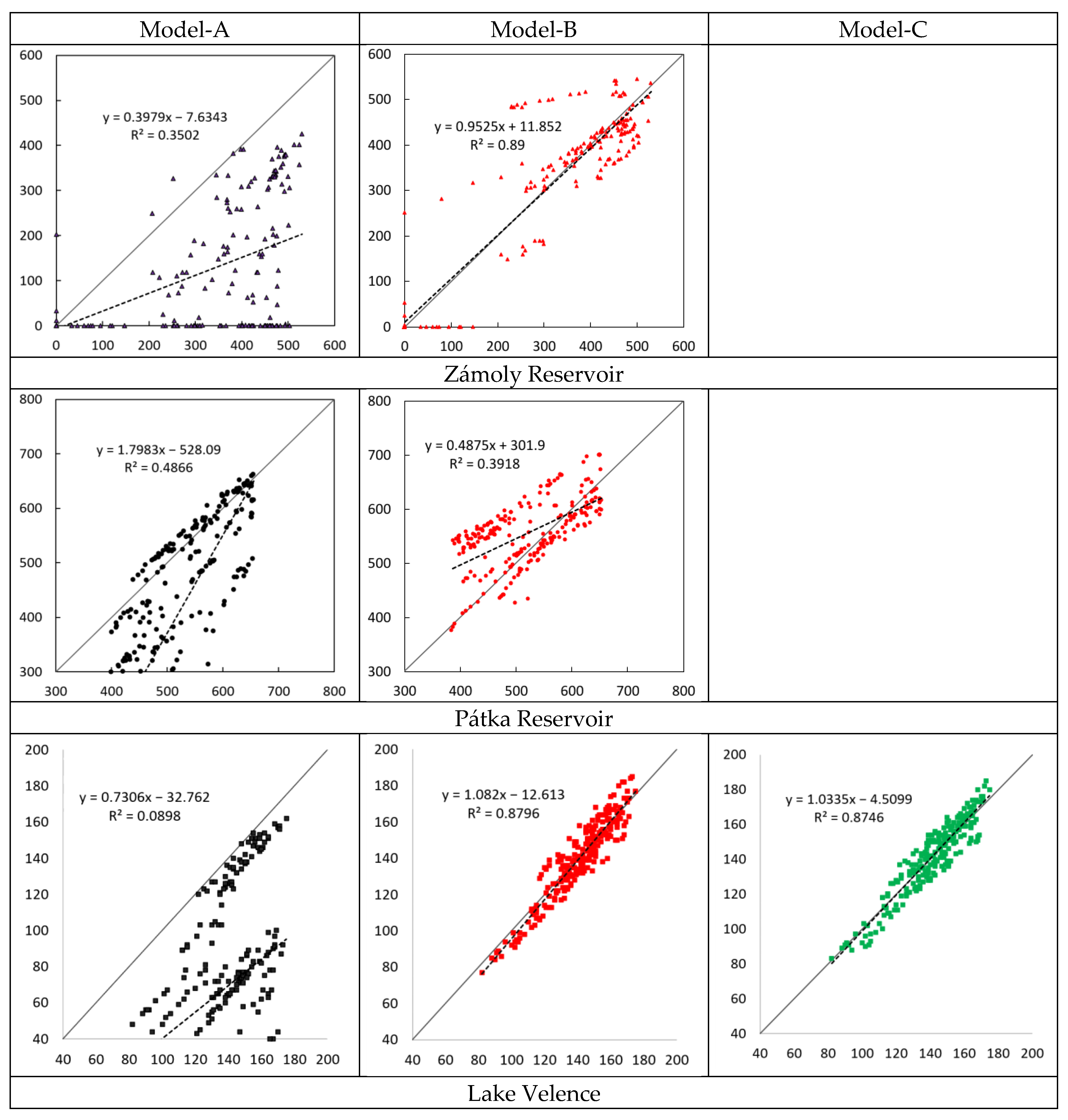
The agreement between the simulated and observed water levels was evaluated using scatter plots, including a 45° reference line and fitted regression lines (Figure 13). The 45° line represents perfect agreement, while deviations from this line indicate bias or scaling errors.

For Model-A, the regression results show substantial deviation from the 45° line, with slopes far from unity and low coefficients of determination. The result indicates both poor representation of variability and significant systematic bias. For Model-B, the regression slopes are close to 1, and intercepts are relatively small, particularly for Zámoly Reservoir (slope ≈ 0.95, R² ≈ 0.89), indicating that both the magnitude and variability in water levels are well reproduced. For Pátka Reservoir, the regression slope remains notably different due to the inconsistency in reservoir outflow for a certain month, as mentioned earlier. For Lake Velence, both Model-B and Model-C show slopes close to unity and high R² values, indicating good agreement with the observed dynamics. However, Model-C further improves the intercept, indicating improved bias correction. Model-C results for the reservoirs are identical to Model-B; therefore, their regression relationships remain identical.

5.5.2. Residual Analysis

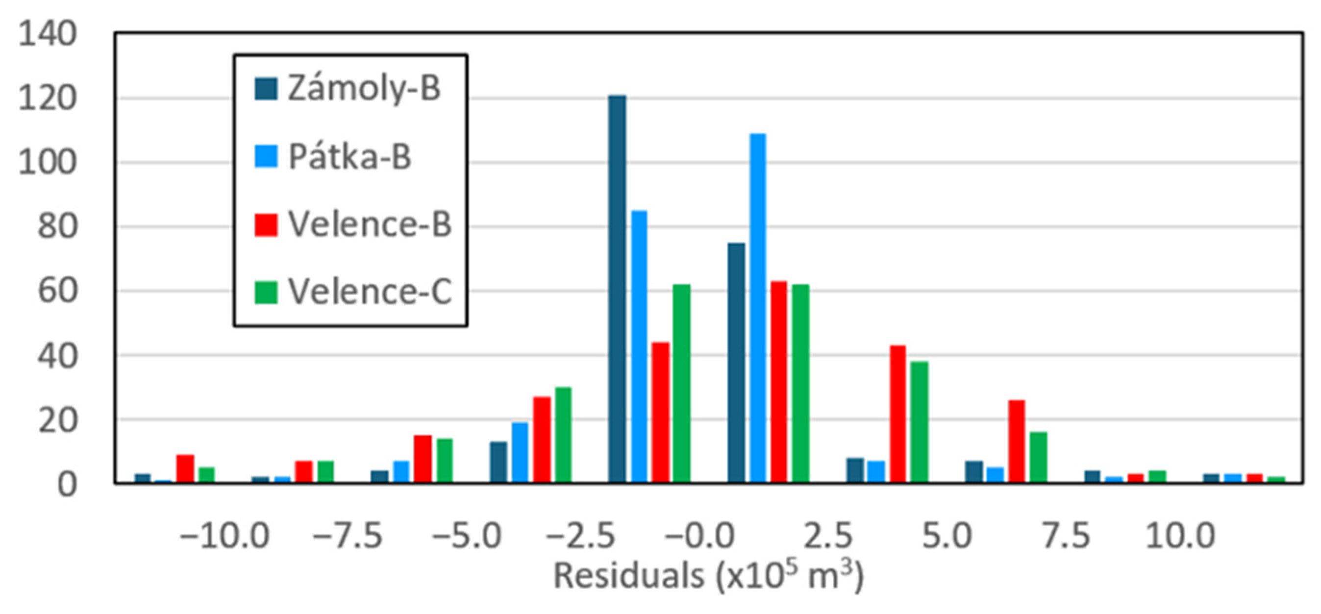
Residual diagnostics reveal clear differences in model performance across water bodies and model formulations. Figure 14 shows histograms of the residuals for Model-B and Model-C. The histograms for Zámoly and Pátka Reservoirs show distributions that are somewhat non-normal. The Zámoly data contain a significant number of zero values (317/444) for the time period studied (see Figure 9). The histograms for Lake Velence show a more normal distribution with Model-C.

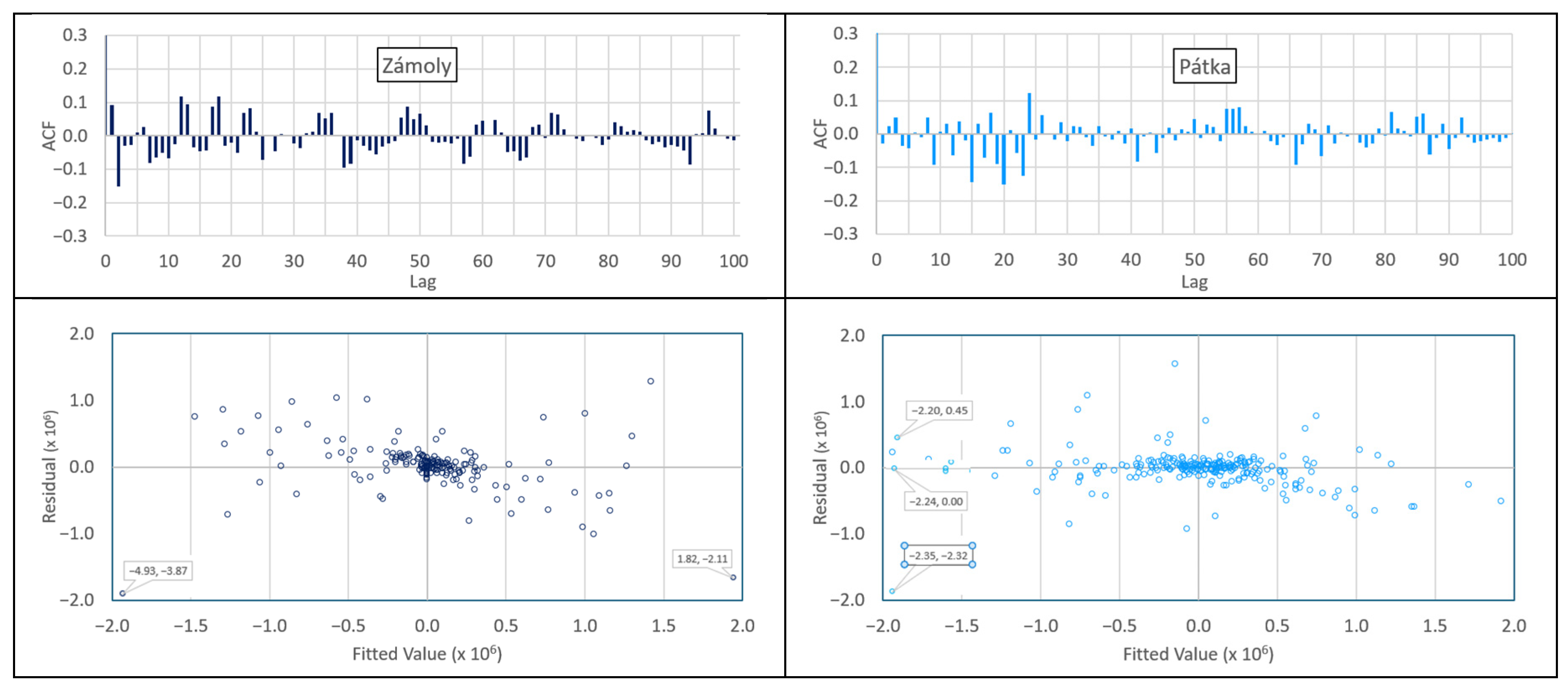
Figure 15 shows the autocorrelation functions (ACFs) and distribution of residuals for Zámoly and Pátka Reservoirs. Zámoly Reservoir exhibits some periodicity in its autocorrelation results; however, the ACF magnitude is modest. The Pátka Reservoir results show no pattern and low magnitudes. The residual distributions follow the same pattern, with Zámoly showing heteroscedasticity: negative fitted values yield positive residuals, and positive values yield negative residuals. Pátka presents a more random distribution; however, residuals may tend to increase with increasing fitted values, but the distribution is generally homoscedastic.

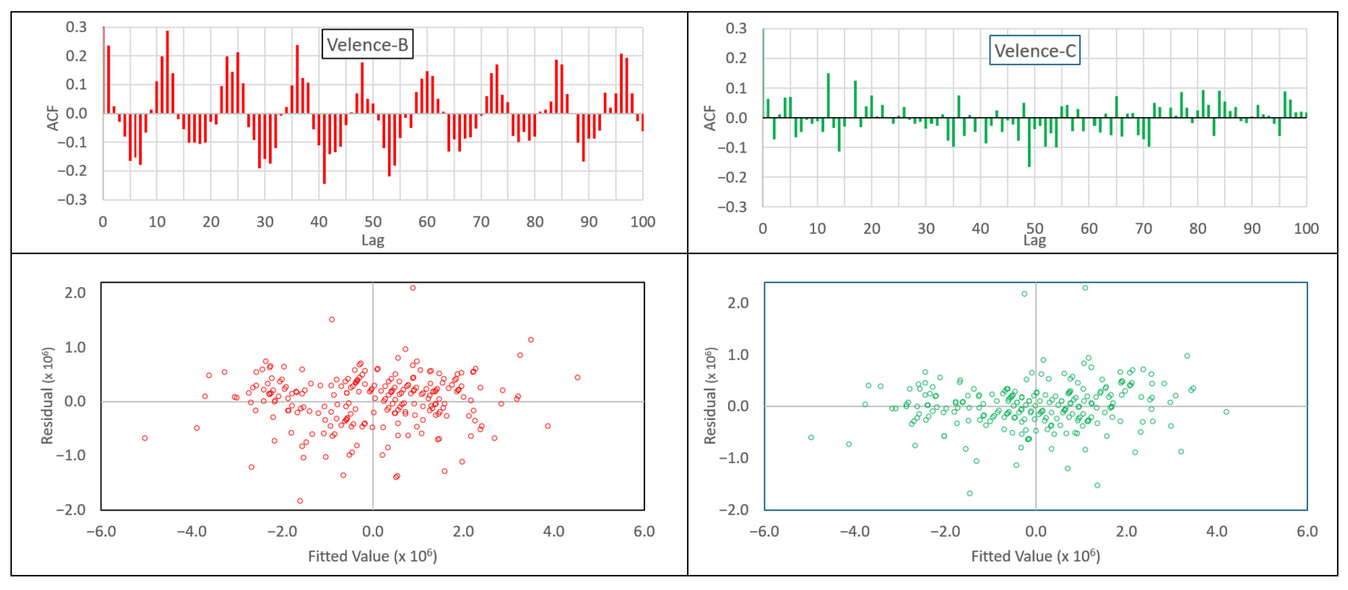
In contrast, the residuals for Lake Velence under Model-B are homoscedastic and closer to normality, but they exhibit autocorrelation, indicating temporal dependence. Model-C leads to a substantial improvement in residual behavior for Lake Velence. Residuals become more normally distributed, autocorrelation reduces significantly, and variance remains consistent over time, indicating homoscedasticity. Residual analyses for Lake Velence are shown in Figure 16.

5.6. Validation Results (2018–2024)

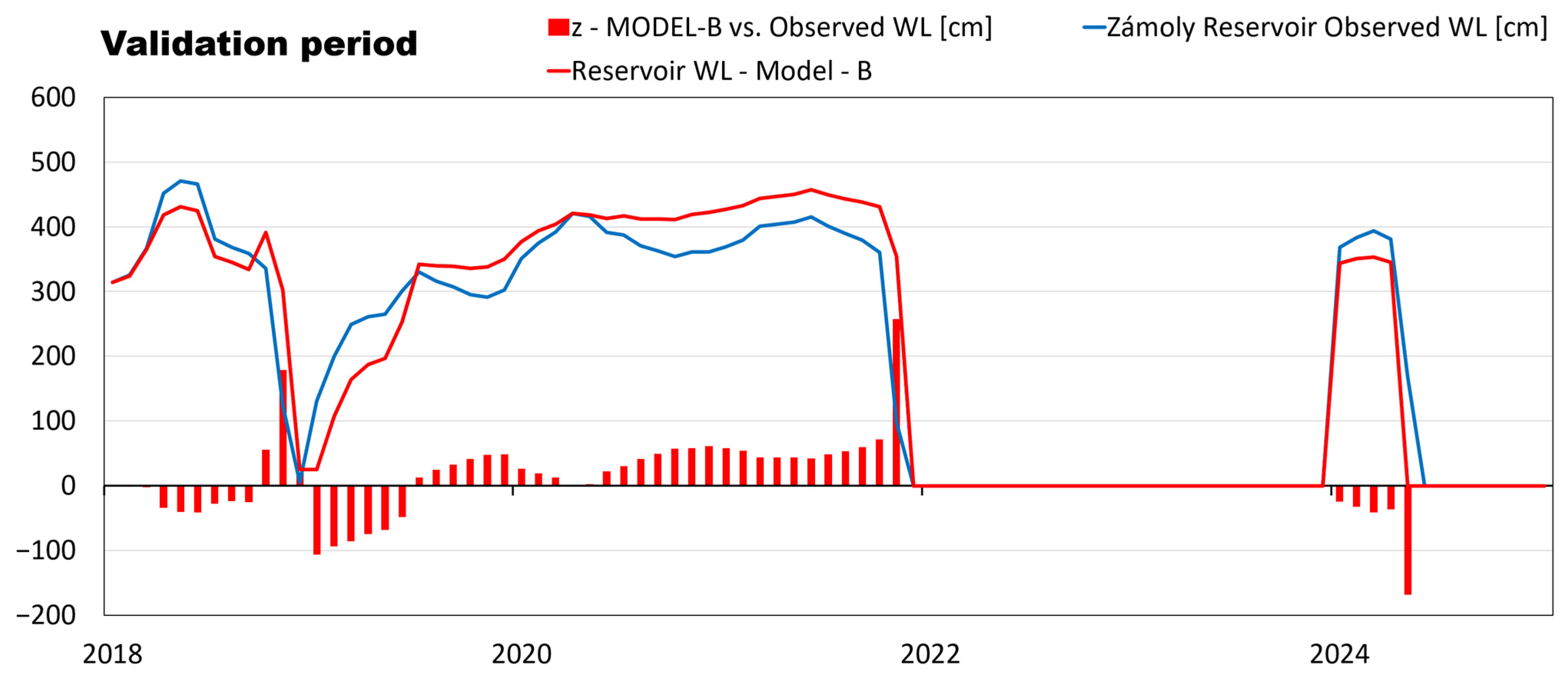
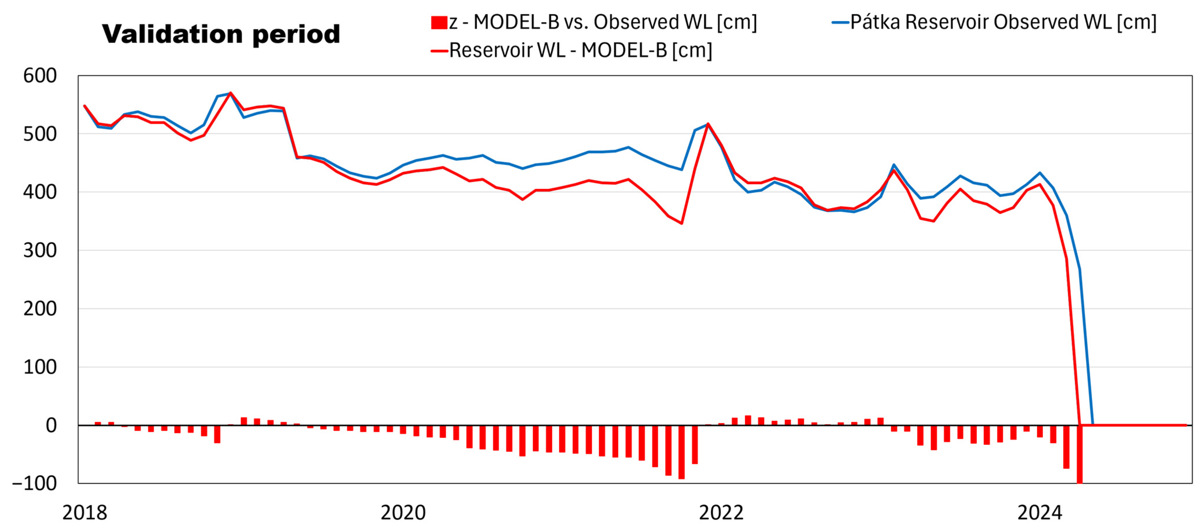
Model performance was evaluated on an independent validation period (2018–2024). For the reservoirs, Model-B produced outstanding results, exceeding the calibration results. For Zámoly Reservoir, NSE^B_ZR-valid = 0.91, and for Pátka Reservoir, NSE^B_PR-valid = 0.92.

The observed and simulated water level time series are shown in Figure 17 for Zámoly Reservoir and in Figure 18 for Pátka Reservoir.

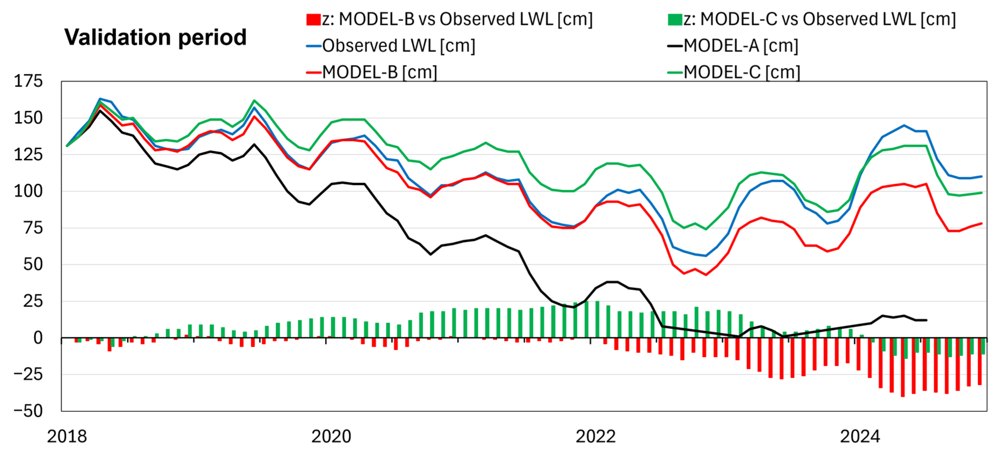
For Lake Velence, Model-C outperformed Model-B (Figure 19): for Model-B, NSE^B_LV-valid = 0.60, and for Model-C, NSE^C_LV-valid = 0.72.

The validation results highlight a key difference between Model-B and Model-C. While Model-B achieves a strong fit during the initial part of the validation period, its performance deteriorates under changing hydrological conditions, indicating limited robustness. In contrast, Model-C provides more stable performance across the entire validation period, with reduced long-term drift. The better performance suggests that accounting for seasonal bias improves model performance under non-stationary conditions. The improved validation results of Model-C are consistent with the residual analysis and support the hypothesis that temporally structured errors are a dominant source of uncertainty in the system.

The results show a clear progression in model performance. Model-A diverges due to cumulative bias, Model-B stabilizes the system through global correction, and Model-C further improves consistency by addressing the seasonal error structure.

6. Discussion

The results demonstrate that the water balance of the cascaded reservoir–lake system is affected by systematic and distributed errors rather than purely random variability. This conclusion is supported by the failure of Model-A, which results in physically unrealistic water levels within a relatively short period. Such behavior indicates that the assumption of zero-mean residuals is violated and that systematic biases are present in the input data. A key observation is that these errors cannot be attributed to a single component but instead arise from inconsistencies across multiple water balance terms, including inflow, precipitation, evaporation, and reservoir releases. The multiple terms are particularly evident in Zámoly Reservoir, where measured outflows substantially exceed the sum of inflows and precipitation minus evaporation. This imbalance suggests unmeasured inflows, uncertainties in discharge measurements, or structural limitations in the monitoring network. The relatively large correction applied to inflow-related coefficients in Model-B further supports the interpretation that inflow underestimation plays a major role in the observed discrepancies.

An important outcome of this study is the demonstration that errors propagate both temporally and spatially within cascaded hydrological systems. In such systems, inaccuracies introduced in upstream components are transmitted downstream through reservoir releases, thereby affecting all subsequent elements of the cascade. This mechanism explains the observed differences in model performance between the three water bodies. The upstream Zámoly Reservoir shows the best agreement after correction. At the same time, performance deteriorates at the intermediate Pátka Reservoir and then stabilizes again at Lake Velence due to the buffering effect of its larger storage capacity. These results highlight that water balance errors are not isolated but are dynamically transferred through the system. This finding extends previous studies that focused primarily on individual lakes or reservoirs and underscores the need for system-level approaches to address water balance closure in interconnected systems.

The application of multiple linear regression as a bias correction tool significantly improves model performance and stabilizes long-term simulations. However, the regression coefficients should not be interpreted solely as empirical fitting parameters. Instead, they provide insight into the underlying inconsistencies within the water balance components. Coefficients deviating from unity indicate the presence of systematic measurement errors, missing processes, or structural deficiencies of the initial water balance model. For instance, elevated coefficients associated with inflow suggest that measured inflows underestimate actual water contributions, while deviations in precipitation coefficients may reflect spatial representativeness issues or methodological limitations.

In contrast, evaporation coefficients remained consistently close to unity across all calibrated models, indicating that the evaporation estimates were generally reliable and required only minor adjustment. This consistency suggests that evaporation contributes less to the observed water balance errors than precipitation or inflow estimates. In this sense, the regression-based correction serves not only as a modeling tool but also as a diagnostic framework for identifying uncertainties in the input data.

One of the most significant findings of the study is the identification of a pronounced seasonal pattern in water balance errors, with systematic deviations occurring primarily during the December–May period. The improved performance of Model-C confirms that these errors are temporally structured and cannot be adequately addressed using time-invariant correction factors. The seasonal behavior suggests the influence of processes not fully captured by the current water balance formulation, including seasonal biases in precipitation measurements, potential groundwater interactions, and/or operational effects of reservoir management.

The role of precipitation uncertainty deserves particular attention. Spatial variability of rainfall across the catchment may introduce systematic bias when a limited number of stations are used to represent basin-wide conditions. Kebede et al. [43] reported similar findings that spatial rainfall gradients can lead to overestimation of lake levels when not properly accounted for. For Lake Velence, the weak negative correlation between precipitation and residual error suggests that precipitation inputs may be underestimated during wetter periods. However, precipitation bias alone cannot explain the magnitude and seasonal structure of the observed water balance deficit.

A more plausible explanation involves an unobserved groundwater component. As highlighted by Dorigo et al. [9], a water balance cannot be accurately closed if one or more components are missing. The groundwater modeling results of Baják et al. [37] provide strong evidence for this, indicating a net groundwater inflow of approximately 47 lake mm/year. This magnitude is comparable to the observed long-term annual error and would substantially reduce the imbalance if included in the water balance equation. The omission of groundwater exchange, therefore, represents a major limitation of the current modeling framework. The absence of an explicit groundwater term has important implications for interpreting the MLR-based correction coefficients as well. In the present model, regression coefficients implicitly compensate for missing or biased components, including groundwater fluxes. As a result, the calibrated coefficients represent aggregated corrections rather than purely physical scaling factors. Explicitly incorporating groundwater would likely reduce the magnitude of these corrections and improve the model’s physical interpretability while allowing a clearer distinction between measurement error and actual hydrological processes.

Residual diagnostics provide further insight into model adequacy. Model-B residuals exhibit heteroscedasticity, deviations from normality, and temporal autocorrelation, particularly for Lake Velence. These characteristics indicate that important processes remain unresolved and that model assumptions are only partially satisfied. The introduction of seasonal correction in Model-C significantly improves residual behavior by reducing autocorrelation, stabilizing variance, and bringing residuals closer to normality. These results confirm that seasonality is a key driver of model error structure.

The findings confirm that water balance closure in regulated systems cannot be achieved solely through the direct use of measured data. Instead, systematic errors embedded within multiple components must be addressed simultaneously. The proposed methodology provides a practical framework for achieving this by combining physical consistency with data-driven correction.

Despite these improvements, several limitations remain. The model does not explicitly account for groundwater exchange, and the regression-based correction does not provide a comprehensive physical explanation for the observed discrepancies. In addition, model performance depends on the quality of input data and the accuracy of reservoir operation records. Future research should focus on integrating groundwater fluxes, exploring probabilistic or Bayesian approaches for uncertainty representation [11], and combining regression-based correction with conceptual hydrological models. Although the present study demonstrates the applicability of the proposed methodology for reconstructing a consistent water balance, an explicit assessment of parameter uncertainty and sensitivity would be a valuable prerequisite before applying the calibrated models to evaluate alternative reservoir operation scenarios, as it would allow the robustness of management decisions to be quantified.

Overall, the proposed approach provides a scalable and operationally applicable method for closing the water balance in cascaded systems. By correcting systematic biases and ensuring consistency across connected water bodies, the methodology enables more reliable long-term simulations and supports the development of water management scenarios.

7. Conclusions

This study presented a data-driven methodology for constructing and closing the joint water balance of a cascaded reservoir–lake system using long-term monthly observations. A baseline water balance model based on uncorrected measured data (Model-A) was first implemented, followed by two bias correction approaches using multiple linear regression (Model-B and Model-C).

The results demonstrate that applying measured water balance components directly leads to significant cumulative errors, rendering the baseline model unsuitable for long-term simulation. These discrepancies arise from the combined effect of systematic errors across multiple components rather than from a single dominant source. The application of MLR correction with uniform coefficients across all months (Model-B) substantially improves model performance and stabilizes the simulated water level time series across all water bodies. However, residual analysis reveals that model errors exhibit temporal structure, particularly at the lake. Incorporating this seasonal behavior (Model-C) further improves model consistency by reducing autocorrelation and improving residual characteristics, resulting in more reliable long-term simulations.

The findings highlight that water balance closure in cascaded systems requires a system-level approach that accounts for both spatial connectivity and temporal variability of errors. The proposed framework provides a transparent and computationally efficient method for correcting systematic biases while preserving the information contained in measured time series.

Despite these improvements, limitations remain, particularly regarding the representation of groundwater exchange and other unobserved processes. Future work should focus on integrating additional physical components and on exploring probabilistic approaches to represent uncertainty explicitly.

Overall, the developed methodology enables the reconstruction of consistent water balance time series and provides a robust foundation for subsequent water management scenario analysis in regulated and interconnected lake and reservoir systems.