Article

How Spatial Resolution of Soil Information Affects Hydrological Modeling in More Complex Topography—A Comparison for a Mesoscale Mountainous Watershed in NE Tanzania


1
Institute for Integrated Management of Material Fluxes and of Resources (UNU-FLORES), United Nations University, 01067 Dresden, Germany
2
Institute of Soil Science and Site Ecology, Faculty of Environmental Sciences, TUD Dresden University of Technology, 01737 Tharandt, Germany
3
Department of Agriculture, Earth & Environmental Sciences, Mwenge Catholic University, Moshi P.O. Box 1226, Kilimanjaro, Tanzania
4
Department of Wildlife Management, College of African Wildlife Management, Mweka, Moshi P.O. Box 3031, Kilimanjaro, Tanzania
*
Author to whom correspondence should be addressed.
Hydrology 2026, 13(5), 124; https://doi.org/10.3390/hydrology13050124
Submission received: 26 February 2026 / Revised: 26 April 2026 / Accepted: 1 May 2026 / Published: 4 May 2026
(This article belongs to the Section Soil and Hydrology)

Abstract

Integrated watershed management relies on distributed hydrological models to simulate water transport processes and support decision-making. However, model reliability is often constrained by the resolution and quality of input data, particularly soil information. High-resolution soil datasets remain scarce in many regions of Sub-Saharan Africa, limiting the representation of spatial soil heterogeneity in hydrological simulations. This study evaluates the effect of detailed soil information derived using the Soil–Land Inference Model (SoLIM) on the performance of the Soil and Water Assessment Tool (SWAT) in the Sigi River watershed, a topographically complex watershed in northeastern Tanzania. Two model setups were compared: (i) a high-resolution SoLIM-based soil dataset and (ii) the coarser global ISRIC SoilGrids database. The SoLIM-informed model better reproduced hydrographs and flow duration curves and showed stronger parameter sensitivities, achieving superior calibration performance (NSE = 0.87, PBIAS = 8.7%) compared to SoilGrids (NSE = 0.86, PBIAS = 11.1%). Hydrological component analysis further revealed that SoLIM enhanced baseflow (181 vs. 60 mm/year) and percolation (349 vs. 135 mm/year) while reducing surface runoff (263 vs. 474 mm/year). These findings demonstrate that high-resolution soil data measurably improve the representation of subsurface processes and moderately improve streamflow performance, especially for baseflow and low-flow regimes; reduce model uncertainty; and improve the robustness of SWAT simulations, thereby supporting more effective watershed management in data-scarce and heterogeneous landscapes.

1. Introduction

Distributed models are crucial for effective integrated watershed management, as they provide essential insights into hydrological processes, ecological interactions, and human impacts on water resources [1]. They help watershed managers to identify problems, evaluate options, and develop adaptive strategies to address environmental issues while balancing socio-economic and environmental needs, thereby enhancing sustainability and resilience [2]. However, limitations and inaccuracies in model inputs hinder effective watershed management. These issues often result from insufficient data inputs, such as terrain, climate, land use, and soil [3,4].
In particular, soil plays a critical role in water transport processes as it controls infiltration, runoff formation, and water storage, making water available for plants, which minimizes surface evaporation and maximizes water use efficiency [5,6,7,8,9,10]. Despite its importance, high-resolution soil information, particularly at the small and meso watershed scales, is often scarce [11]. This scarcity is a widespread issue, as spatial soil information is frequently incomplete or insufficient in many regions worldwide, i.e., Sub-Saharan Africa [4]. The primary reasons for this situation include the time-consuming, labor-intensive, and costly nature of conventional soil survey [2,12,13]. Additionally, despite advancements in satellite-based systems, accurately capturing relevant soil properties through remote sensing remains challenging [11]. This limitation leads to significant challenges for hydrological assessment and sustainable land management, as critical soil characteristics such as soil depth, texture and related hydraulic properties are essential for streamflow generation and water balance [2,14]. Spatial variation in these properties also plays a crucial role in determining the spatially variable soil moisture regimes and evapotranspiration rates in a watershed.
Digital soil mapping has emerged as a technique to overcome the issue of soil information scarcity across the globe. Ref. [15] developed a prototype soil observation database for global soil mapping in Indonesia, outlining the steps needed to prepare legacy soil data for digital mapping while addressing challenges related to inadequate spatial soil data, i.e., in developing countries. This ultimately can provide insights for better soil data management too. Currently, high-resolution soil mapping can be achieved through advanced digital mapping techniques like the Soil–Land Inference Model (SoLIM), which applies the third law of geography, stating that similar geographic environments exhibit similar features [16]. In particular, the model utilizes environmental covariates such as moisture index, slope, and curvature to map soils and create a soil database. Refs. [13,14] used the SoLIM model to generate high-resolution soil data for the implementation of the SWAT model [17,18] to mesoscale watersheds in order to simulate streamflow.
Several studies have analyzed the impact of soil data resolution on the performance of the SWAT model [4,11,12,19,20,21]. Ref. [19] found that the spatial resolution of the global soil database leads to a high uncertainty of SWAT model outputs. Ref. [11] concluded that while the quality and resolution of soil data affect all components of the hydrological cycle, particularly soil water (SW) and water yield (WYLD), they do not cause significant discrepancies in WYLD simulation, especially after model calibration. Ref. [4] found that using finer-resolution soil data, such as those from DSOLMap, improved the daily streamflow simulation of the SWAT+ model both before and after calibration and validation. Ref. [13] demonstrated that using high-resolution SoLIM-generated soil data in SWAT yields more realistic simulations of initial peak flow events after the dry season. These results were attributed to the improved resolution of soil data, which provided a detailed spatial representation of soil properties such as depth, texture, bulk density, hydraulic conductivity, and organic carbon content [8]. It is known that these properties govern processes such as infiltration, water storage, and percolation, which are crucial for runoff formation. For instance, soils with higher infiltration rates and greater water-holding capacity can significantly affect the timing and magnitude of runoff and peak flows, especially during dry season transitions [5,6,10,22,23,24]. Low-resolution soil data, which aggregate these properties over larger spatial units, fail to capture this variability, leading to oversimplification of soil–water interactions and higher uncertainty in model predictions. However, conclusions regarding the effects of soil data resolution remain inconsistent across studies, as the magnitude of improvement depends strongly on dominant soil types and landscape characteristics such as topography and land cover, and these effects remain largely unexplored in tropical mountainous watersheds where soil data scarcity is most pronounced.
This study addresses a critical gap in hydrological modeling research in Tanzania, where the influence of input data, particularly soil data, on hydrological predictions has been minimally explored. Most previous studies have focused on applying the SWAT model without adequately assessing how uncertainties in input data propagate into key hydrological components that underpin water-related risks. As a result, the implications of soil data quality for simulating runoff generation, baseflow, and sediment transport remain poorly understood, despite their importance for drought assessment, flood response, and reservoir management, as these processes are strongly controlled by soil depth, texture, and hydraulic properties that are poorly represented in coarse global soil datasets. To address this gap, this research examines the effect of high-resolution soil data on SWAT model performance in the Sigi River watershed in northeastern Tanzania, a less-studied watershed characterized by complex topography and diverse land use/cover patterns across elevation gradients [25]. These landscape features contribute to strong spatial variability in soil properties. The basin also experiences severe soil erosion, leading to sedimentation and siltation in a downstream reservoir that is critical for the water supply of the metropolitan area of Tanga, Tanzania’s second-largest harbor [26,27]. Long-term discharge and climate records, together with recently collected local soil data, provide a unique opportunity to assess how improved soil representation influences hydrological simulations. Our study addresses the following questions: (1) To what extent do the key soil properties required by the SWAT model differ between the high-resolution SoLIM dataset and the generalized SoilGrid dataset? (2) How do the resolution and quality of soil input data influence the performance and predictive accuracy of the SWAT model in simulating hydrological processes?

2. Materials and Methods

2.1. Study Area

The Sigi River watershed is located in NE Tanzania (5°12′ S and 38°36′ E; 4°48′ S and 38°70′ E) (Figure 1). The elevation ranges from 90 to 1200 m asl. The watershed covers most of the East Usambara Mountains and their foothills [25]. At the outlet of the Mabayani Reservoir, for which the watershed has been delineated, it has an area of 887 km2. The region is characterized by a humid tropical climate with bimodal rainfall occurring from March to May and October to December. A dry season typically occurs from January to February, bridging the short and long rainy periods. Rainfall ranges from 1540 mm in the upland plateau (Amani station) to 1173 mm close to the reservoir dam (Lanconi station), with temperatures spanning from 20 °C to 27 °C [28,29]. The E Usambaras are characterized by old crystalline rocks, which have weathered to nutrient-poor, sandy–loamy and mostly acidic soils (predominantly Acrisols: [29,30,31]). Above an elevation of 850 m, soils are highly leached and quickly depleted by farming. In contrast, lower altitude soils, including those on escarpments and in lowlands, are richer in nutrients and more suitable for agriculture [30]. Alluvial valleys, like those of the Sigi R., contain nutrient-rich Fluvisols, ideal for farming. The study area showcases a diverse range of land uses, including primary and secondary forests, shrubland, and various plantations such as teak, other trees, tea, and sisal [25]. Small-scale cultivation is prevalent, alongside citrus and spice agroforestry practices. Built-up areas, grasslands, and areas dominated by rocks are also present, reflecting a mix of natural and agricultural landscapes. Land use and land cover vary notably with elevation: the uplands are dominated by forests, small-scale farms, tea plantations and spice agroforestry systems [25,31]; the foothill escarpments are characterized by small-scale cultivation, citrus agroforests, and teak plantations; while the lower coastal plain areas are mainly occupied by small-scale cultivation and citrus agroforests [25].
Since Tanzania’s independence in the 1960s, extensive forest and shrubland in the Sigi River watershed have been converted to agricultural land leading to increased sediment loading and declining water quality in the downstream reservoir [25,26,28]. This transformation has resulted in a 38% decrease in the reservoir’s storage volume since its construction, with the primary cause being the loss of vegetation and adverse soil management practices upstream jeopardizing water-related ecosystem services [26]. Forest cover was observed to decline between 1955 and 1996 [25,26], likely contributing to increased soil erosion and siltation, while efforts such as Sustainable Land Use Management (SLM) have been limited by the use of coarse-resolution land use and soil inputs in SWAT, reducing the model’s ability to inform effective adaptive land management strategies.

2.2. Digital Soil Mapping

The Soil–Land Inference Model (SoLIM) was applied to newly delineate soil units and develop a more detailed soil property database for the study area. SoLIM was selected for its ability to generate detailed, spatially continuous soil maps through fuzzy logic and environmental similarity, making it particularly suitable where field observations are sparse. SoLIM is a predictive digital soil mapping tool that leverages the spatial relationship between soil properties and environmental variables to create likelihood maps [32,33]. Grounded in the third law of geography, which states that locations with similar environmental characteristics tend to have similar soil properties, SoLIM infers soil attributes in areas with limited data by using known soil characteristics and their correlation with environmental factors. The model integrates two types of knowledge: typical soil occurrence conditions and how similarity changes as conditions deviate [32].

2.2.1. Data Sources and Processing

The environmental covariates used in this study included a 30 m resolution Shuttle Radar Topography Mission (SRTM) digital elevation model (DEM), which was obtained from the United States Geological Survey (USGS) through the Earth Explorer platform (http://earthexplorer.usgs.gov/). From the DEM, secondary terrain attributes such as humidity index, slope, profile curvature, and contour curvature were extracted. In addition, land use/land cover data were taken from [25].
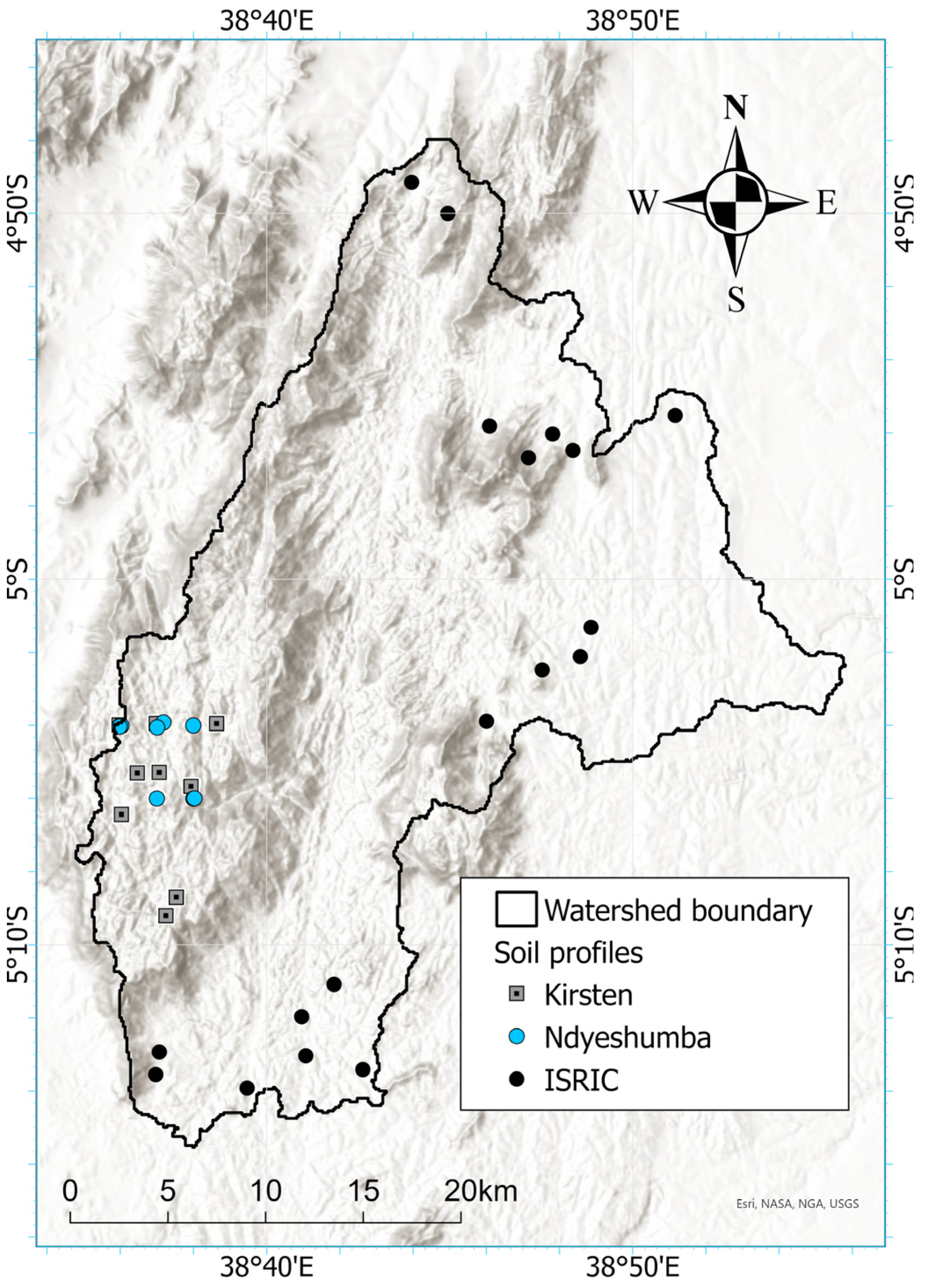
For soil data, 36 soil profiles in the Sigi River watershed were gathered from the literature (Figure 2, Table 1). Each contains information on soil physical properties such as texture, bulk density (BD), and soil carbon content. This dataset combines legacy soil profile data from [34], who studied soil property variations along slopes in the Amani sub-catchment to assess land use suitability, and [29], who quantified soil organic carbon stocks in the E Usambara Mts. across different land use and land cover conditions. Additionally, the dataset includes standardized soil profiles from the ISRIC World Soil Information archive, collected mostly between the 1960s and 1990s, providing a valuable historical context for spatial distribution of soil characteristics [35]. For the purpose of data harmonization, the soil profiles were conceptually divided into four depth intervals, 0–25 cm, 25–50 cm, 50–75 cm and 75–100 cm, using the equal-area quadratic spline depth function method as used by [15,36].
To generate soil property maps in SoLIM, a sample-based approach was applied, modeling and predicting soil properties based on relationships between environmental covariates and observed soil characteristics. The information on the soil properties of the selected 36 soil profiles was combined with environmental factors such as elevation, wetness index, slope, profile curvature, contour curvature, and land use/land cover as inputs to the SoLIM model. Using these inputs, SoLIM calculates similarity scores (Sij) between known and unknown soil locations, following the method described by [32], as shown in Equation (1):
S i j = P ( E ( e 1 i , e 1 j ) , E ( e 2 i , e 2 j ) , E ( e x i , e x j ) , E ( e y i , e y j ) )
where (Sij) represents the environmental similarity between unvisited location (i) and sample location (j); (exi) and (exj) are the values of the xth environmental covariate at these locations; and y is number of environmental covariates used. Functions E() and P() calculate environmental similarity at the covariate and soil sample scales, respectively, based on methods from [32]. The similarity score quantifies how closely the environmental variables at a known sampling point match those at an unvisited location. By extending this relationship spatially, the SoLIM model infers soil properties across the study area.
Then, a fuzzy membership map (i.e., continuous similarity map) was created based on soil properties to produce the soil mapping units (SMUs). The soil at each location is represented by a “soil similarity vector”, reflecting degrees of resemblance to various soil properties. By calculating these similarity values for every pixel, SoLIM produces a set of fuzzy membership maps, where each map shows the spatial distribution of a particular SMU. A more detailed explanation can be found in [37,38]. The fuzzy membership map in SoLIM was refined by assigning each pixel to the SMU with the highest membership value, creating a discrete “hardened” SMU map. This analysis was done using SoLIM Solutions 2015 software, version 5.

2.2.2. Validation of SoLIM Soil Map

Validation of the SoLIM-derived soil map was conducted using independent soil observations and model-derived uncertainty information. A subset of field soil profiles was withheld from model training and used exclusively for validation. Predicted soil classes were compared with observed soil classes at these locations to assess the agreement between mapped and field-based soil information.
Prediction uncertainty was further evaluated using the uncertainty outputs generated by the Soil–Landscape Inference Model (SoLIM) during soil class mapping. SoLIM employs a fuzzy logic framework to quantify the similarity between environmental covariates and soil–landscape rules derived from training samples, producing spatially explicit uncertainty values for each grid cell [19,32]. These uncertainty values express the confidence associated with each soil class prediction and were used to support the validation framework and guide interpretation of map reliability.
The combined use of independent validation samples and spatial uncertainty layers formed the basis for evaluating the quality and robustness of the soil map prior to its application in watershed-scale hydrological modeling.

2.3. Integration of SoLIM Data in SWAT

For the hydrological model, we selected the Soil and Water Assessment Tool (SWAT) [17,18]. The purpose was to examine how the difference in resolution and spatial distribution of soil types, particularly soil maps generated by the SoLIM, affects the model’s performance. SWAT is a semi-distributed, process-oriented model designed by the USDA to assess the effects of land management on water flows, sediment transport, and export of chemicals in complex watersheds. The model divides the watershed into sub-basins and hydrologic response units (HRUs) based on unique combinations of soil, land use, and slope [17,18]. In SWAT, soil information is crucial for simulating various hydrological processes and related flow rates which are essential for accurately addressing the effects of different land management practices on watershed dynamics.

2.3.1. Data Acquisition and Processing

A 30 m resolution Shuttle Radar Topography Mission (SRTM) digital elevation model (DEM) was utilized to extract key watershed delineation parameters, including the humidity index, slope, profile and contour curvatures, and the river network, using an automated model. Land use and land cover (LULC) data were derived using a Landsat image from 2022 based on [25]. Climate data (daily precipitation and air temperature) from 1990 to 2019 were obtained from long-term observations at the stations Amani (911 m asl), Lanconi (121 m asl), Marikitanda (975 m asl), Mlingano (205 m asl), and Longuza (165 m asl) provided by the Tanzania Meteorological Agency. Observed daily streamflow (discharge) data for the same period were taken from the Lanconi gauging station (121 m asl) provided by the Pangani Basin Authority.
A detailed soil map for the mesoscale watershed of the Sigi River is not available currently. Therefore, spatially distributed soil information from SoilGrids (https://soilgrids.org/) was used in our study. The tool was selected because it provides globally consistent, open access soil property estimates at relatively high spatial resolution with standardized depth intervals, making it a widely used reference dataset in hydrological modeling. Its level of detail supports the representation of soil–water interactions, infiltration, and evapotranspiration, while its regular updates and methodological consistency enable robust comparison with locally derived soil datasets, despite limitations in capturing fine-scale soil heterogeneity. The soil datasets used include the SoilGrids data at a scale of 250 m, developed by ISRIC and accessed through https://soilgrids.org/ as well as the soil dataset generated using SoLIM (Section 2.2).

2.3.2. SWAT Model Setup

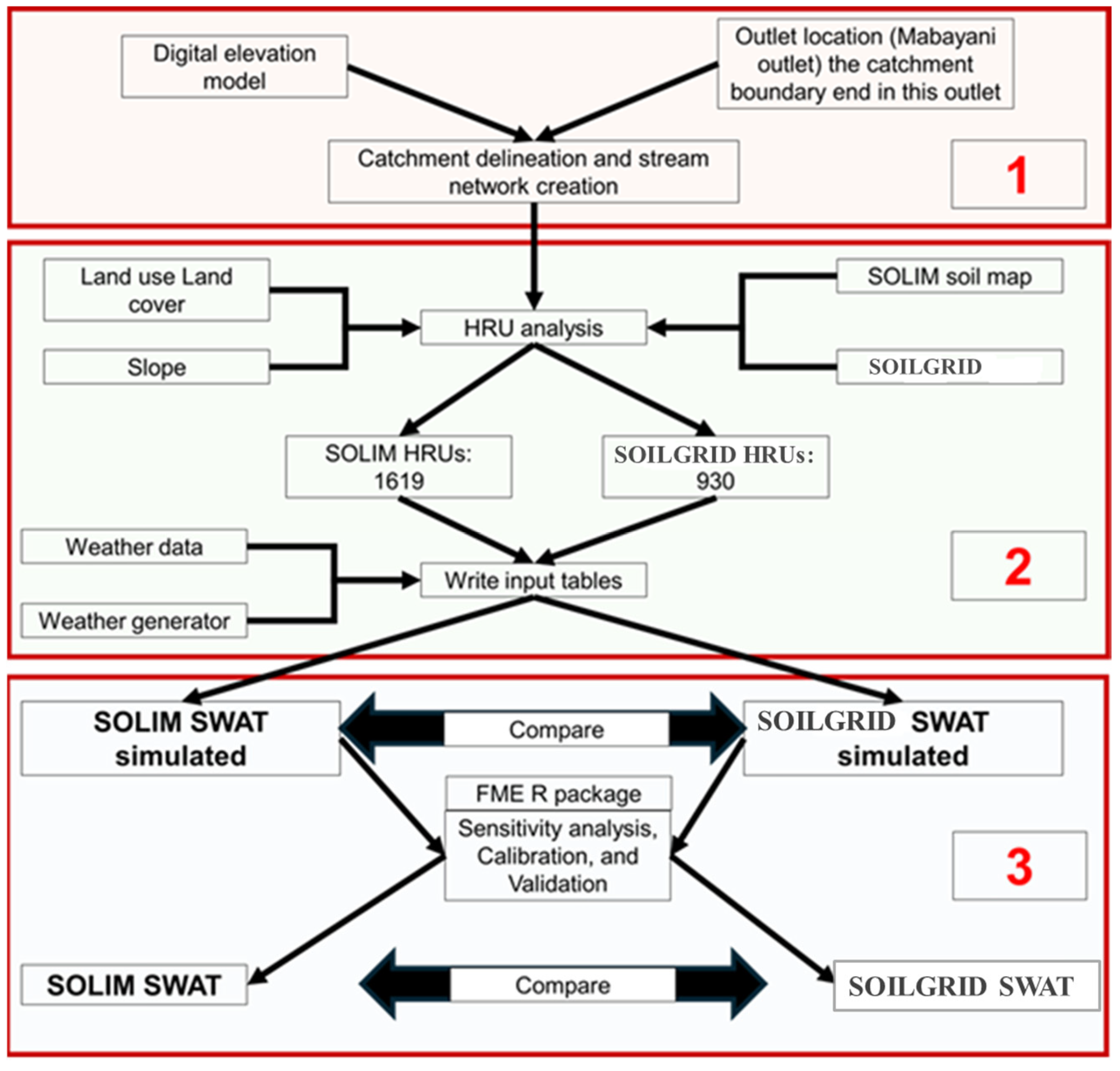
Figure 3 describes the workflow for SWAT model setup and simulation. It consists of three main steps: (1) delineate the Sigi River watershed; (2) run the SWAT model using the SoLIM-based soil map (scenario 1) and SoilGrids soil map (scenario 2) as model inputs for comparison; and (3) perform sensitivity analyses, calibration, and validation in both scenarios. In this study, model setup was conducted using QSWAT version 1.6.3.
The Sigi River watershed was delineated using a 30 m resolution digital elevation model (DEM) to define its boundaries and stream network. SWAT utilized the DEM to identify drainage patterns and divided the watershed into sub-watersheds. This process ensures accurate simulation of hydrological processes and serves as the basis for further analyses. As a result, a watershed area of 887 km2 was delineated, and 108 sub-watersheds were identified.
The watershed and sub-watershed delineations were used to set up two SWAT models, using two different soil scenarios (SoLIM and SoilGrids) to generate HRUs. The SWAT model uniformly simulates water flows and underlying vegetation and soil processes within each HRU. Before generating HRUs, adjustments were made to the plant growth module based on [39] to improve the SWAT model’s simulation of perennial vegetation dynamics under growth conditions in the tropics. HRUs were then generated by overlaying land use, soil, and slope data within each sub-watershed without applying any threshold, resulting in 1619 HRUs for the SoLIM scenario and 930 HRUs for the SoilGrids scenario, with the difference attributed to the higher resolution of the SoLIM map. Both models incorporated the same daily climate data for the period 1990–2019, including temperature, precipitation, relative humidity, wind speed, and solar radiation, enabling the generation of daily outputs at the HRU and sub-watershed scales. To minimize the impact of initial conditions, a 6-year warm-up period (1990–1996) was used, followed by a 22-year simulation period (1997–2019). This approach ensured a more accurate simulation of hydrological processes and water discharge for the Sigi River watershed.
Models are mostly associated with significant uncertainties arising from experimental design, input data and parameter [40]. The sensitivity analysis was performed separately for two SWAT model scenarios, one using the SoLIM-derived soil map and the other using the SoilGrids map. The global sensitivity analysis method, which uses multivariate linear regression with parameters generated through uniform Latin Hypercube Sampling, similar to the Sequential Uncertainty Fitting algorithm (SUFI-2) [41], was applied. The parameters selected for sensitivity analysis (Table 2), commonly used for streamflow calibration, were taken from study [39]. Three objective functions, namely Nash–Sutcliffe efficiency (NSE), coefficient of determination (R2), and probability bias (PBIAS) as described by [42] for streamflow, were used to assess model responses to changes in the parameters.
For model calibration, Separate Automated Latin Hypercube Sampling (LHS) was conducted for the two scenarios using the FME package in R to generate 3000 parameter sets as done by [39], with the parameters being the most sensitive ones obtained in the sensitivity analysis. Model performance for both scenarios was evaluated using NSE, R2, and PBIAS [42] over the 1997–2007 period, with validation conducted for 2008–2019. This approach enabled the comparison of model performance and sensitivity to the two different soil input scenarios.
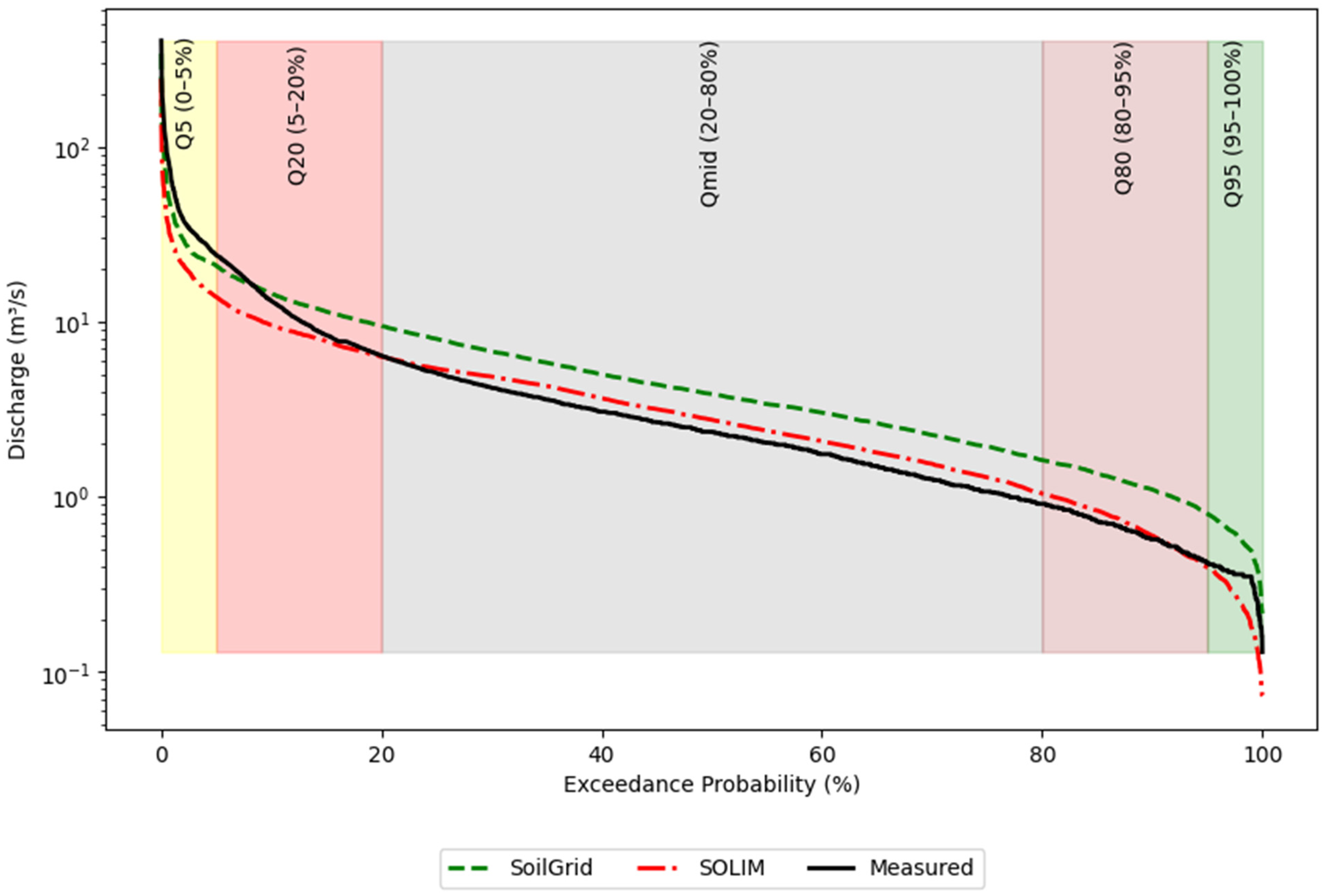
Further analysis was conducted to evaluate how SoLIM and SoilGrids map scenarios differ in simulating high and low flow events using flow duration curves (FDCs) constructed using the HydroGOF package [39]. Each FDC was divided into five segments (5FDC) following [39,43]: very high flows (0–5%, Q5), high flows (5–20%, Q20), medium flows (20–80%, Q50), low flows (80–95%, Q80), and very low flows (95–100%, Q95).

3. Results

3.1. SoLIM-Derived Soil Data: Spatial Distribution and Characteristics

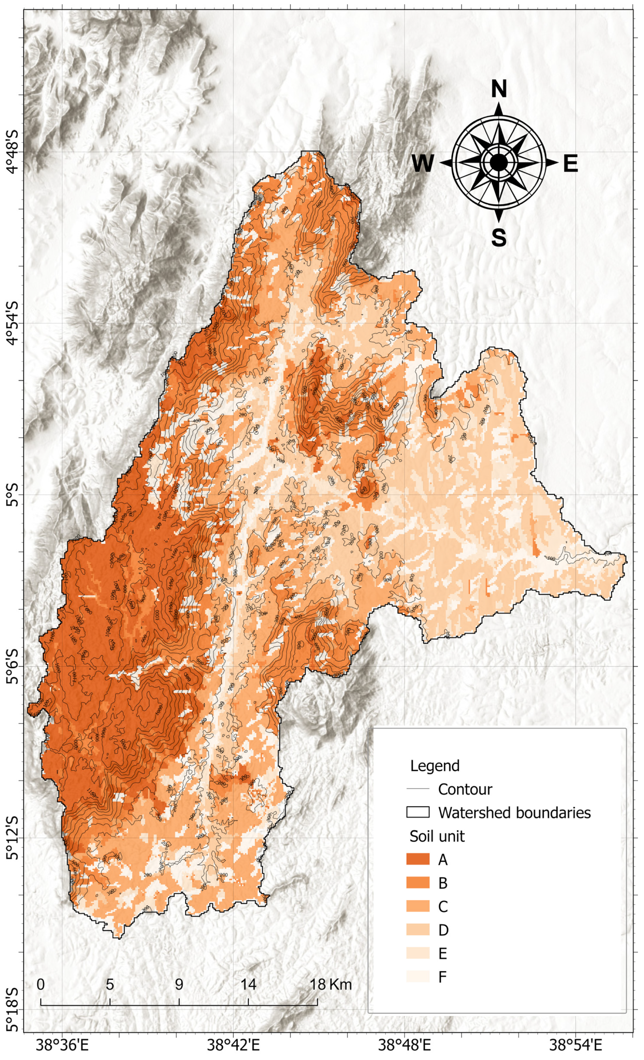
The application of SoLIM for the Sigi River watershed resulted in the delineation of six distinct soil units. The map in Figure 4 shows their spatial distribution. In Table 3, the key physical properties of the six soil units are given. Their respective shares of areas in the watershed vary between 10 and 20%. Unit A was characterized by moderate BD (1.05–1.22 g/cm3) and relatively high AWC (0.18–0.34 cm3/cm3) in the subsurface layers. Values for saturated hydraulic conductivity (K) were low to moderate (6–19 mm/h), while SOC declined sharply with depth, from 2% at the surface to 0.7% at 75–100 cm. Unit B is characterized by higher clay contents (50–68%) and correspondingly lower sand contents, resulting in lower rates of K (3–21 mm/h) but increased water retention (AWC up to 0.35 cm3/cm3 in deeper layers). Bulk density (BD) ranged from 1.03 to 1.21 g/cm3, remaining relatively stable across depths. Unit C contrasted strongly, with a loamy texture dominated by sand (46–55%) and moderate clay (20–24%). This resulted in relatively uniform BD values (1.25–1.33 g/cm3) and lower water-holding capacities (AWC 0.16–0.22 cm3/cm3). K values were modest (8–15 mm/h), while SOC remained low (1.1–1.5%). Unit D, with clay contents of 34–46%, displayed rather low K (1–10 mm/h) and very low AWC (0.10–0.17 cm3/cm3), consistent with its compact structure (BD up to 1.27 g/cm3). Values of SOC were moderate (0.55–1.42%) in the topsoil. Unit E represented the most heterogeneous soil group: while the surface horizon had relatively low clay (14%) and high sand (74%), deeper layers became progressively finer textured (clay up to 40%). This variability translated into a wide range of water-holding capacities (AWC 0.13–0.23 cm3/cm3) and K (6–28 mm/h). Notably, the topsoil carbon contents reached 3.16%, the highest among all units. Unit F, in contrast, was dominated by coarse texture (sand contents 75–82%) and very low clay contents (<10%). This sandy texture resulted in the highest K of all units (50–70 mm/h) but also the lowest water retention (AWC 0.07–0.10 cm3/cm3). BD increased with depth (1.17–1.33 g/cm3).
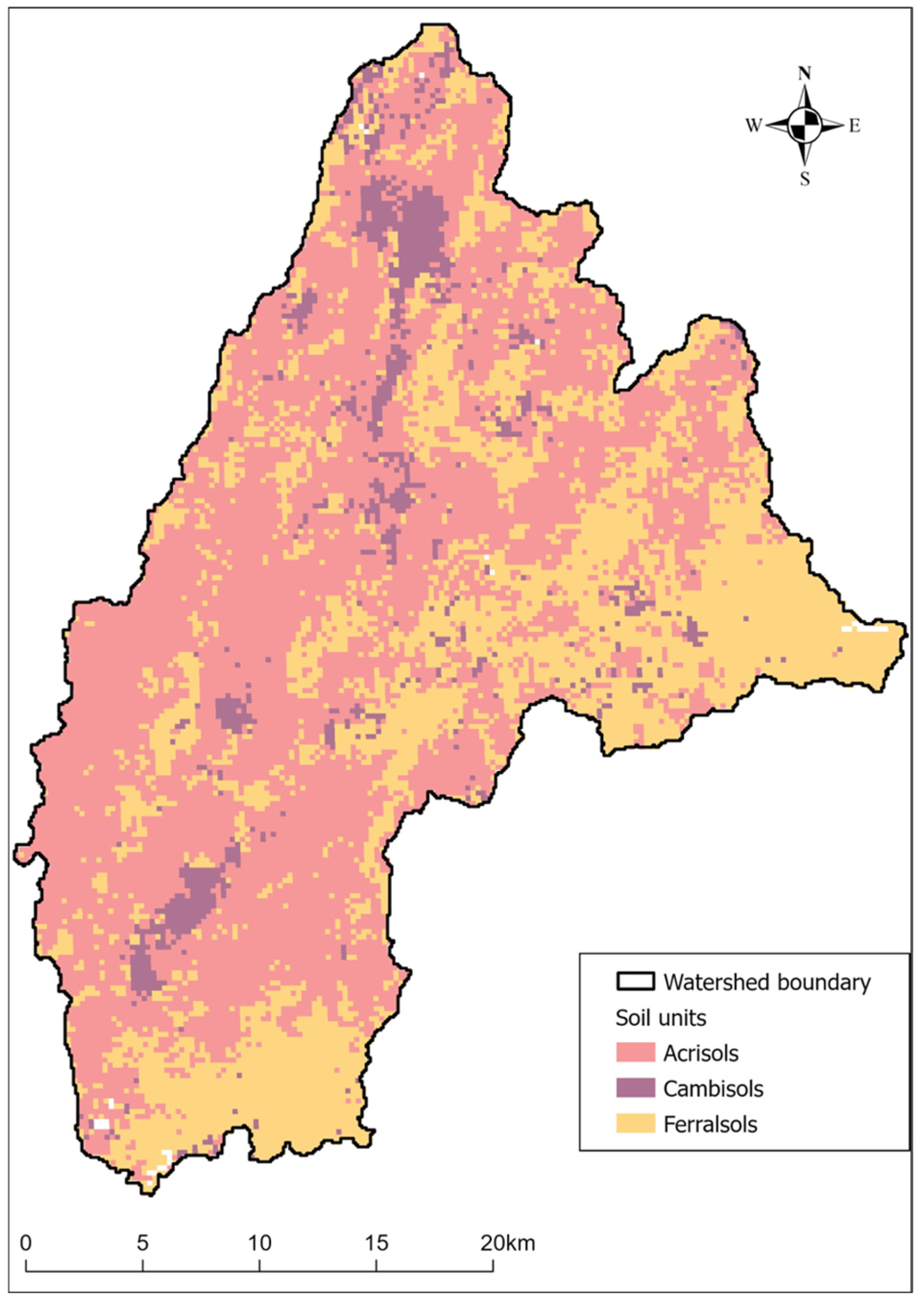
SoilGrids yields three major soil units for the Sigi River watershed: Acrisols, Ferralsols, and Cambisols. The map in Figure 5 shows their spatial distribution in the watershed. In Table 4, the corresponding numbers for the four depth intervals are given. The Acrisols (at 64%, they are by far the dominant soil unit in the watershed) had BD values increasing with depth from 1.35 to 1.48 g/cm3, with AWC gradually decreasing from 0.18 to 0.15 cm3/cm3. K values were relatively low, between 5 and 10 mm/h. Clay contents increased from 40% at the surface to 45% at depth, while SOC declined from 1.2% to 0.3%. Ferralsols were characterized by BD values of 1.30–1.42 g/cm3, with AWC decreasing from 0.20 to 0.16 cm3/cm3. K ranged from 3 to 8 mm/h. Clay content was consistently high, increasing from 55% in the surface to 62% in the deepest layer, while SOC declined from 1.0% to 0.3%. Cambisols showed BD values from 1.32 to 1.45 g/cm3 and AWCs ranging from 0.21 to 0.16 cm3/cm3. K decreased from 12 mm/h at the surface to 6 mm/h in the subsoil. Clay content increased with depth, from 25% at the surface to 32% at 75–100 cm, while SOC decreased from 1.0% to 0.4%.

3.2. Accuracy and Uncertainty of the SoLIM-Derived Soil Map

To evaluate the performance of the SoLIM-derived soil map at the soil unit level, predicted soil classes were compared with observed classes at independent validation locations. The accuracy assessment was quantified using the agreement coefficient (AC), alongside error-based metrics adapted to categorical comparison, and supported by the standard deviation (SD) of observed class distribution. The SoLIM soil map achieved an overall agreement coefficient of 0.76, indicating good correspondence between predicted and observed soil units. The classification error, expressed as mean absolute disagreement, was 0.24, suggesting that approximately 76% of soil units were correctly identified. The variability in observed soil unit distribution (SD = 0.28) indicates moderate heterogeneity across the watershed, within which the model predictions fall.
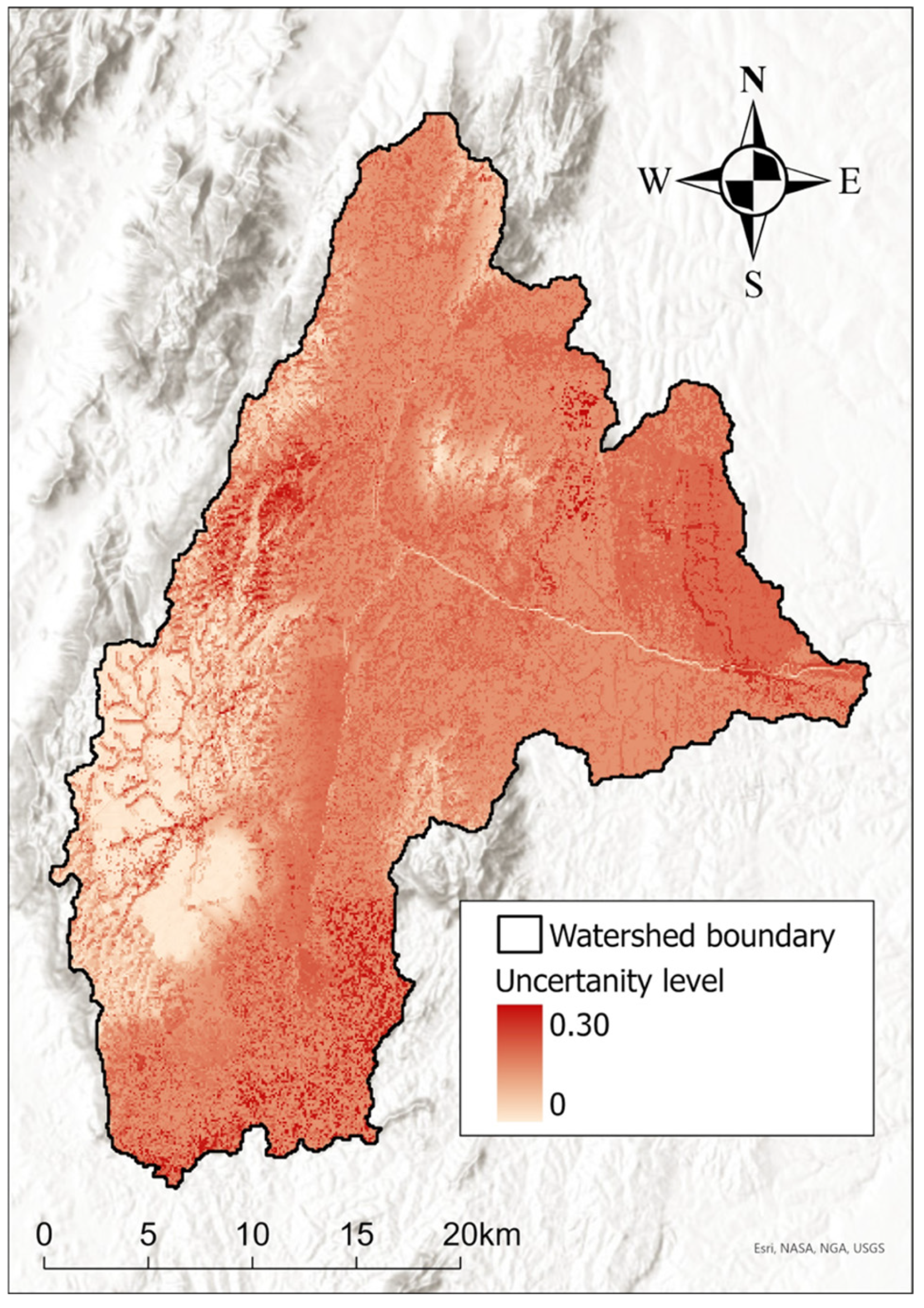
The spatial distribution of prediction uncertainty derived from the SoLIM model is shown in Figure 6. Uncertainty values range from 0 to 0.30, where lower values indicate higher confidence in soil class assignment based on the degree of similarity between environmental covariates and soil–landscape rules. Across most of the watershed, uncertainty values are low to moderate with localized zones of elevated uncertainty likely associated with heterogeneous terrain conditions or limited training data coverage, with large areas exhibiting values close to zero. Higher uncertainty values (approaching 0.30) occur in spatially limited clusters, particularly in zones characterized by complex topography. These patterns indicate spatial variability in prediction confidence, with localized areas exhibiting reduced certainty relative to the surrounding landscape.

3.3. SWAT Performance Before Calibration and Validation

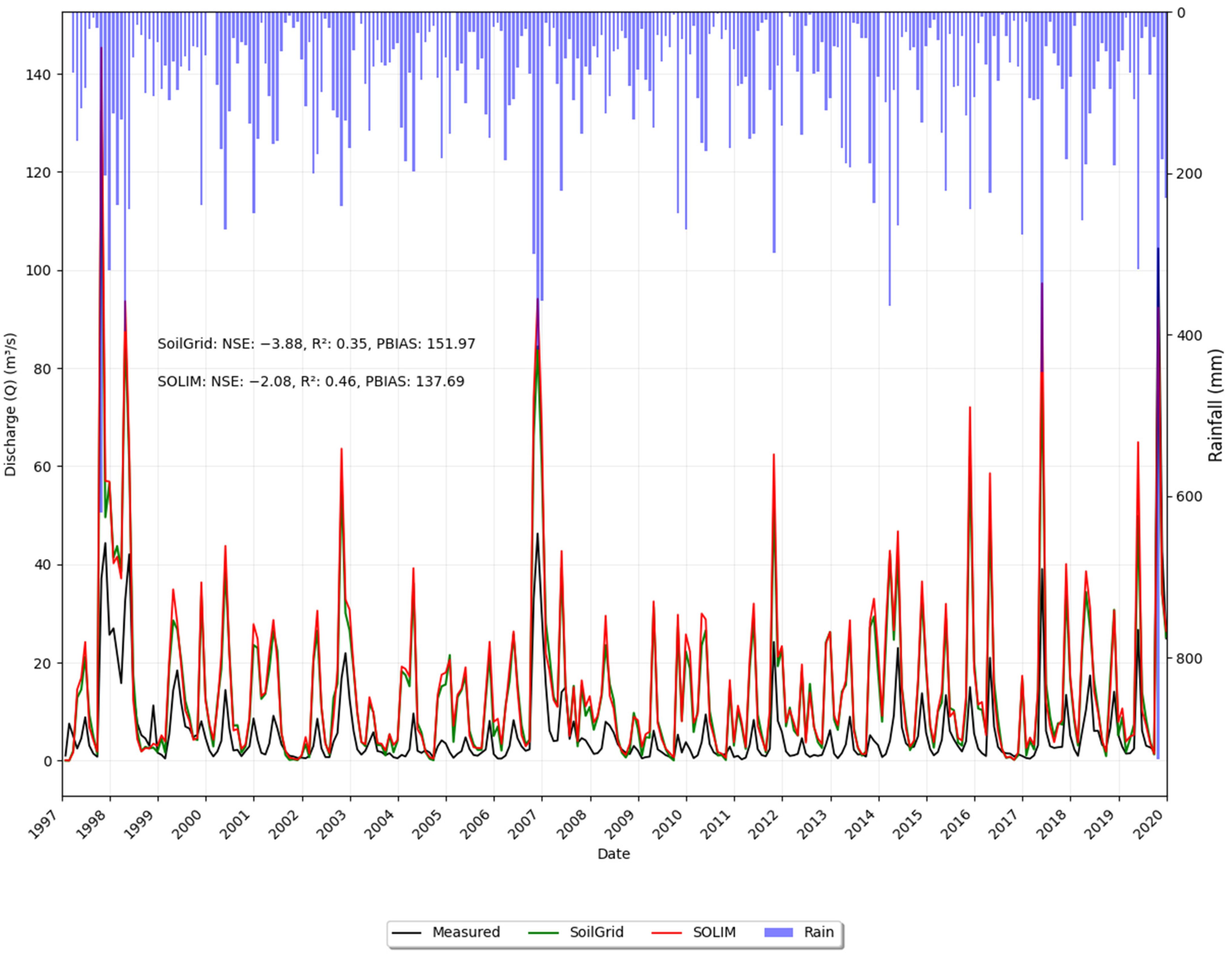
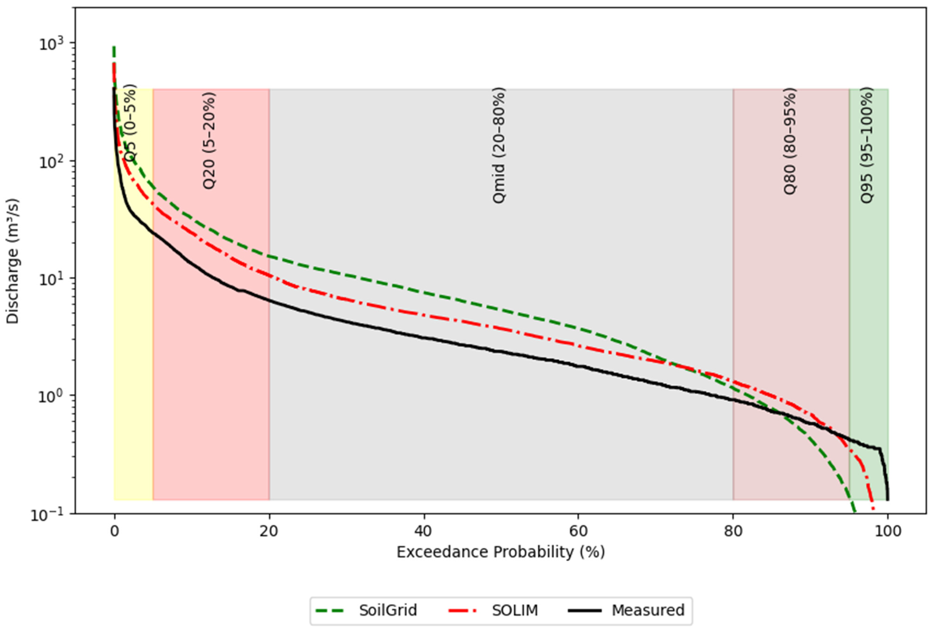
In Figure 7, the temporal comparison between observed and simulated streamflow using different soil datasets is presented. This demonstrates a clear effect of soil resolution on the performance of streamflow simulation in SWAT. Before calibration and validation, the SoLIM map enables the model to more closely align the seasonal and inter-annual variations with observed streamflow than the low-resolution SoilGrid. A comparison of the two hydrographs underlines that the SoLIM map (red line) better captures the overall temporal dynamics of discharge compared to the SoilGrids map (black line), particularly during high-flow events. The statistical metrics indicate that the SoLIM map outperforms the SoilGrids map, achieving higher Nash–Sutcliffe efficiency (NSE; −2.08 and −3.88, respectively) and coefficient of determination (R2; 0.46 and 0.35, respectively). The SoLIM-based model accurately estimates the timing and magnitude of both high and low flows (Figure 8). The figure illustrates the ability of each soil dataset to reproduce the full spectrum of streamflow conditions at the watershed outlet, including low-flow behavior and peak-flow events. The FDC demonstrates how well each soil map captures the full range of streamflow conditions, from low flows to flood events. It reinforces these findings, demonstrating that the SoLIM map aligns more closely with observed measured discharge (green dashed line) across all flow regimes, especially during high flows (Q0–Q5%), mid-range flows (Q20–Q80%), and extremely low-flow conditions (Q80–100%). Meanwhile, the SoilGrids map exhibits greater overestimation, highlighting its limitations in accurately capturing low-flow dynamics.

3.4. SWAT Performance After Calibration and Validation

A sensitivity assessment of both calibrated SoLIM and SoilGrid SWAT models for the Sigi River watershed revealed significant variations in how SWAT parameters affected model performance when comparing the SoLIM and SoilGrid-based models. The curve number (CN2.mgt) emerged as the most influential parameter in both scenarios, though SoLIM showed stronger sensitivity (t-stat: 45.96) compared to SoilGrid (t-stat: 33.76). The SoLIM-based model consistently resulted in high parameter sensitivities, including Manning’s roughness coefficient (CH_N2.rte: 7.49 vs. 6.01) and soil hydraulic conductivity (SOL_K.sol: 6.67 vs. 5.00) (Table 5).
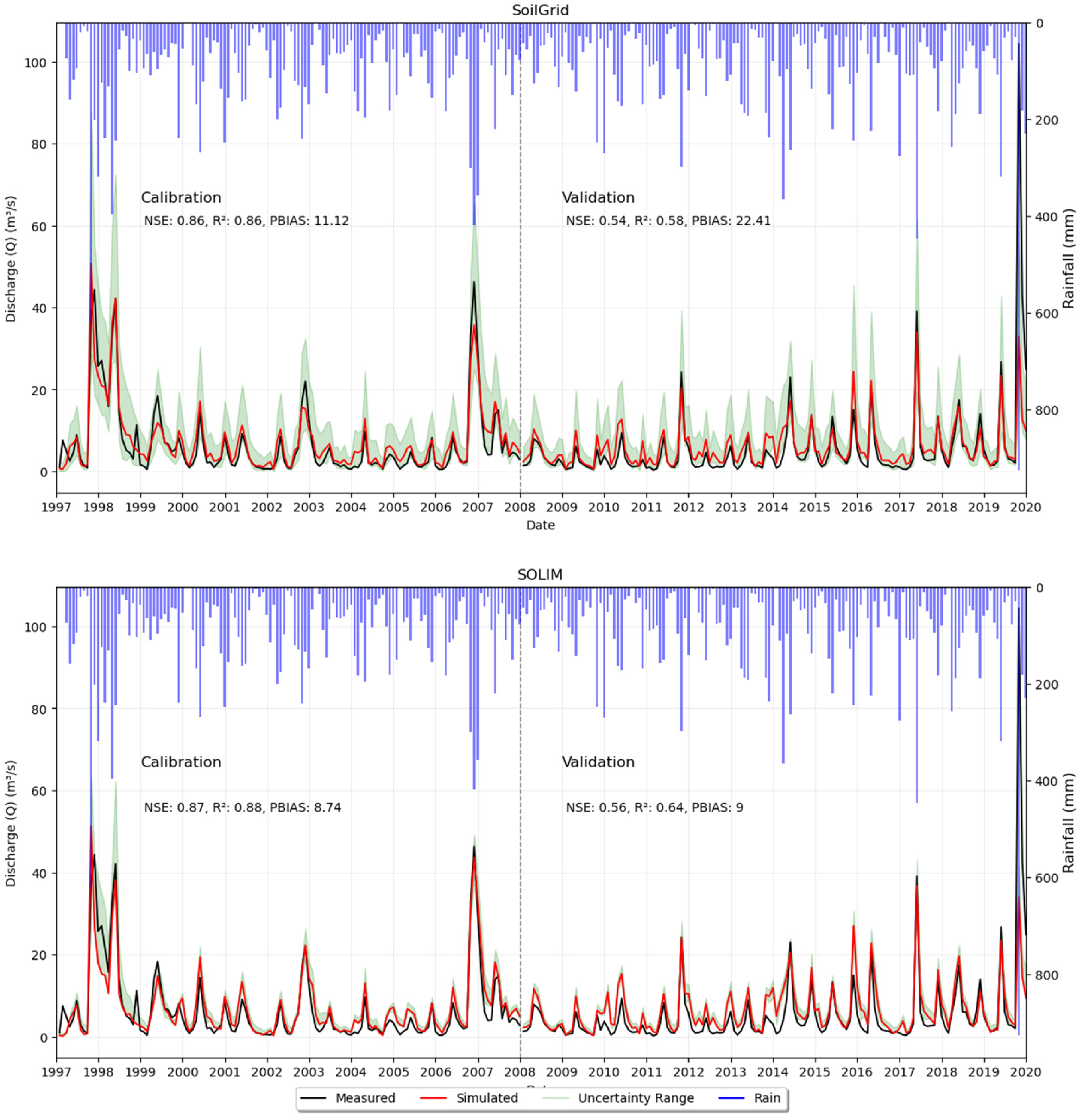
Figure 9 compares the measured and modeled streamflow dynamics of the Sigi River across various soil data scenarios during both the calibration and validation periods. The results highlight the enhanced performance of the SoLIM-based model in simulating seasonal and inter-annual variations in streamflow over the SoilGrid scenario. The SoLIM map had a narrower uncertainty range than the SoilGrid map, which underscores its reliability in capturing hydrological variability. The SoLIM map consistently has higher performance in terms of the overall temporal dynamics of discharge compared to the SoilGrid map, particularly for high-flow and low-flow events. The statistical metrics demonstrate that the SoLIM map outperforms the SoilGrid map during both calibration and validation periods, achieving a Nash–Sutcliffe efficiency (NSE) of 0.87 and a Percent Bias (PBIAS) of 8.74%. In contrast, the SoilGrid scenario performed less favorably, with an NSE of 0.86 and a PBIAS of 11.12%. Peak flow simulations were notably more accurate with the SoLIM map, reducing overestimation by up to 15% compared to SoilGrid, which overpredicted discharge during extreme events by as much as 25%. Similarly, low-flow simulations improved under the SoLIM scenario, reducing underestimations by 20% relative to SoilGrid. Figure 10 illustrates how well each soil dataset can replicate the full range of streamflow conditions at the watershed outlet, including both low-flow behavior and peak-flow events. The flow duration curve (FDC) (Figure 10) supports these findings, showing significant improvements in discharge predictions across all flow regimes when using the SoLIM map. In high-flow conditions (Q5–Q20), the SoLIM model reduced deviations from measured values to below 10%, which was less different from the SoilGrid scenario. For low-flow conditions (Q80–Q95), the SoLIM map demonstrated a 20% reduction in underestimation that outperformed the SoilGrid map, while mid-range flows (Q20–Q80) exhibited a narrower uncertainty band compared to SoilGrid.

3.5. Effects on Hydrological Components

Table 6 presents the annual water balance components simulated by the SoLIM- and SoilGrids-based models. The results show considerable differences between the SoLIM and SoilGrid-based model, highlighting distinct patterns in runoff, baseflow, and percolation. The SoLIM-based model produces greater infiltration and percolation, resulting in substantially higher baseflow and a total water yield driven largely by subsurface processes rather than rapid overland flow. In contrast, the SoilGrids-based model produces a more surface-runoff-dominated system, characterized by limited infiltration, reduced baseflow, and increased surface runoff and evapotranspiration.

4. Discussion

This study examines the effect of soil data resolution on the simulation performance of the SWAT model in a tropical mountainous watershed with complex topography and diverse vegetation cover. We compared the effects of two contrasting datasets derived from (i) SoLIM, which produced high-resolution soil information based on relationships between environmental covariates and soil characteristics from existing profiles in the watershed, and (ii) the globally available SoilGrids data. The significant distinction between these two datasets is not only their spatial resolution but also the level of soil property differentiation they provide, especially for texture, available water capacity (AWC), and saturated hydraulic conductivity (K), which control how rainfall is partitioned into surface runoff, soil storage, and groundwater recharge. Assessing these differences helps clarify the importance of more detailed soil representation on integrated water resource management at the watershed scale, with regard to its effects on the simulation of runoff, baseflow, and sediment transport that are directly relevant to measures for drought risk reduction, flood response, and reservoir management.

4.1. Soil Heterogeneity and Hydrological Implications

Table 3 and Table 4 demonstrate clear differences in how soil information is represented in the SoLIM and SoilGrids datasets. The two datasets differ in the number of soil units delineated within the study area, with SoLIM identifying more units than SoilGrids. Soil properties derived from SoLIM also show substantially greater heterogeneity, presumably better reflecting real soil cover, whereas those from SoilGrids are comparatively homogeneous. The greater number of soil units and the higher variability observed in the SoLIM dataset reflect its finer spatial details and use of locally relevant environmental covariates, which enable improved discrimination of soil conditions [14,33]. In contrast, the globally derived SoilGrids dataset applies to broader spatial generalization that smooths local variability and aggregates soil characteristics into more uniform units [44]. This structural difference influences water partitioning into various water budget components because soil texture and hydraulic conductivity control infiltration, storage, and percolation processes. In the SoLIM dataset, sandy and high-K soils promote rapid infiltration and recharge, while clay-rich or finer soils favor surface runoff generation, creating spatially differentiated flow pathways and baseflow contributions [14]. For example, in our results, SoLIM identifies both very-high-conductivity sandy soils (Unit F) and very-low-conductivity clay soils (Unit D), producing strong spatial contrasts in infiltration capacity, whereas SoilGrids lacks these extremes, helping to explain the reduced infiltration and baseflow simulated under that scenario. SoilGrids tend to reduce hydraulic contrasts by assigning more uniform soil behavior across larger areas, which shifts simulated partitioning toward greater surface runoff and reduced subsurface flow [45]. Conversely, more generalized soil representations may oversimplify runoff generation and subsurface storage patterns, with implications of high uncertainty for simulations of flood response, drought resilience, and reservoir sediment dynamics in heterogeneous catchments. These contrasts underscore the importance of using context-specific and high-resolution soil datasets, particularly in climate-sensitive regions, where a realistic representation of soil heterogeneity is critical for improving predictions of water availability and ecosystem responses and for preparing adaptive mitigation measures.

4.2. SWAT Model Performance and Calibration Dynamics

In the pre-calibration SWAT simulations (Figure 7), clear differences emerged between the two soil datasets. The SoLIM-derived input produced more realistic spatial and temporal streamflow patterns than SoilGrids. This can be attributed to the features of the SoLIM soil map that preserve better spatial differentiations in texture, depth, and hydraulic conductivity across contrasting landscapes, which directly control how rainfall is partitioned into infiltration, storage, and quick runoff before any parameter tuning is applied. As a result, the model starts from a hydrological structure that better reflects actual water flow pathways in the catchment, leading to more credible baseline flow dynamics even before calibration [11,20]. After calibration, the SoLIM-based model more accurately simulated the timing and magnitude of both high and low flows, as shown by the flow duration curve (Figure 10), and displayed a narrower uncertainty range (Figure 9). This performance gain is linked to the stronger physical basis of the finer SoLIM soil inputs, where differentiated hydraulic properties and water-holding capacity across soil units allow SWAT to simulate infiltration, storage, and delayed release more realistically [5,6]. As a result, calibration required fewer parameter adjustments and produced more reliable behavior across discharge conditions, increasing confidence in the model’s representation of hydrological variability and extremes [46]. It is thus assumed that parameter adjustment was more straightforward and intuitive with the SoLIM-based model than with the SoilGrids-based model. This underlines the benefit of using more realistic initial soil parameterization. Although calibration improved the results of both models, the SoilGrids-based model required much stronger adjustments of CN2, SOL_K and ESCO, indicating compensation for incorrect soil structure [46]. This parameter compensation masks structural error and does not correct hydrological partitioning, as reflected by its lower baseflow and distorted FDC shape.

4.3. Soil Effect on Flow Partitioning and Hydrological Components

Differences in simulated water budget components between the SoLIM and SoilGrids scenarios highlight that soil data resolution strongly influences hydrological processes. The SoLIM model produced higher water yield and baseflow and lower surface runoff, which might indicate better representation of infiltration and subsurface storage (Table 6). This behavior reflects the higher K and AWC values assigned by SoLIM to deep, weathered upland soils and alluvial valley soils, which promote infiltration and percolation into shallow and deep aquifers [45]. These patterns likely result from SoLIM’s integration of local terrain and soil variability through fuzzy logic and GIS-based mapping, which captures site-specific hydraulic properties more effectively, governing how water moves through the vadose zone. [33,47]. In the Sigi River watershed, deeply weathered soils at the upper elevations (mostly Acrisols) support deep percolation and delayed runoff, while sandy alluvial soils in valley bottoms allow rapid infiltration but limited storage. [30]. By preserving these contrasts, the SoLIM dataset enables SWAT to route water realistically into both shallow and deep flow pathways. In contrast, SoilGrids smooths these properties across the landscapes, leading to excessive surface runoff on steep slopes and reduced groundwater recharge, which explains the unrealistically low baseflow and high evapotranspiration in this scenario. [4,14]. The lower evapotranspiration predicted by the SoLIM indicates that the SWAT model suggests reduced surface water availability due to more soil water retention, while the modest increase in soil water content further reflects improved representation of soil hydraulic behavior. In contrast, the generalized nature of SoilGrids soil inputs tends to homogenize local variability, leading to a less accurate representation of subsurface storage and lateral flow processes. This limitation leads to an underestimation of baseflow and an overestimation of evapotranspiration in heterogeneous catchments [45,48]. To verify the interpretations of the SWAT model results, a series of validations is required for individual water budget components, such as SoLIM-based ET vs. observed ET, which are lacking in the studied watershed. More observations and measurements should be set up in the future.

5. Conclusions

This study underlines that soil data resolution critically shapes the performance of SWAT as a commonly used watershed model when implemented to a mesoscale mountainous watershed, such as the Sigi River watershed in the humid tropics of Tanzania. High-resolution SoLIM soil information captures fine-scale variability and hydraulic contrasts, enabling more realistic simulations of infiltration, baseflow, and surface–subsurface water partitioning, while coarse global datasets like SoilGrids homogenize these properties, reducing model reliability. Accurate soil representation is essential for assessing dry season water availability, flood response, and sediment delivery to reservoirs, which directly affect water security.
These findings highlight the need for watershed management and policy decisions to account for input data quality: investments in high-resolution soil mapping can improve predictive modeling, support sustainable water allocation, and guide climate adaptation strategies. Future research should evaluate the transferability of detailed soil datasets across similar watersheds. Furthermore, research should integrate refined land use and management scenarios and explore cost-effective approaches for generating local soil information in data-scarce regions. The results demonstrate that improving soil data quality has direct implications for hydrological prediction reliability and for the design of resilient, data-driven watershed management strategies in mountainous tropical regions.

Author Contributions

Conceptualization, S.C., L.Z. and K.-H.F.; methodology, S.C., L.Z. and K.-H.F.; software, S.C., L.Z. and K.-H.F.; validation, S.C., L.Z. and K.-H.F.; formal analysis, S.C., L.Z. and K.-H.F.; investigation, S.C., L.Z. and K.-H.F.; resources, S.C., L.Z. and K.-H.F.; data curation, S.C., L.Z., O.D.K. and K.-H.F.; writing—original draft preparation, S.C., L.Z., O.D.K. and K.-H.F.; writing—review and editing, S.C., L.Z., O.D.K. and K.-H.F.; visualization, S.C., L.Z., O.D.K. and K.-H.F.; supervision, L.Z. and K.-H.F.; project administration, S.C., L.Z., and K.-H.F.; funding acquisition, L.Z. and K.-H.F. All authors have read and agreed to the published version of the manuscript.

Funding

This research was funded by the Saxon State Ministry for Energy, Climate Protection, Environment, and Agriculture (SMEKUL) award number 124219, through a PhD scholarship awarded to the first author.

Data Availability Statement

The data are available from the corresponding author upon reasonable request.

Conflicts of Interest

The authors declare no conflicts of interest.

References

  1. Singh, S.; Mishra, K.; Chavan, R.; Tiwari, H.L. Advancements and Challenges in Hydrological Modeling: A Comprehensive Review; Pandey, M., Umamahesh, N.V., Das, J., Pu, J.H., Eds.; Springer Nature: Berlin/Heidelberg, Germany, 2025; pp. 423–442. [Google Scholar]
  2. Busico, G.; Colombani, N.; Fronzi, D.; Pellegrini, M.; Tazioli, A.; Mastrocicco, M. Evaluating SWAT model performance, considering different soils data input, to quantify actual and future runoff susceptibility in a highly urbanized basin. J. Environ. Manag. 2020, 266, 110625. [Google Scholar] [CrossRef]
  3. Chaplot, V. Impact of spatial input data resolution on hydrological and erosion modeling: Recommendations from a global assessment. Phys. Chem. Earth Parts A/B/C 2014, 67–69, 23–35. [Google Scholar] [CrossRef]
  4. López-Ballesteros, A.; Nielsen, A.; Castellanos-Osorio, G.; Trolle, D.; Senent-Aparicio, J. DSOLMap, a novel high-resolution global digital soil property map for the SWAT + model: Development and hydrological evaluation. CATENA 2023, 231, 107339. [Google Scholar] [CrossRef]
  5. Basche, A.D.; DeLonge, M.S. Comparing infiltration rates in soils managed with conventional and alternative farming methods: A meta-analysis. PLoS ONE 2019, 14, e0215702. [Google Scholar] [CrossRef]
  6. Bens, O.; Wahl, N.A.; Fischer, H.; Hüttl, R.F. Water infiltration and hydraulic conductivity in sandy cambisols: Impacts of forest transformation on soil hydrological properties. Eur. J. For. Res. 2007, 126, 101–109. [Google Scholar] [CrossRef]
  7. Rowley, J. Conducting research interviews. Manag. Res. Rev. 2012, 35, 260–271. [Google Scholar] [CrossRef]
  8. Li, R.; Song, X.; Duan, Z.; Peng, M. Using fuzzy approach to build a continuous relationship between SCS curve number and soil properties. In Proceedings of the 2011 19th International Conference on Geoinformatics; IEEE: New York, NY, USA, 2011; pp. 1–5. [Google Scholar]
  9. Libohova, Z.; Seybold, C.; Wysocki, D.; Wills, S.; Schoeneberger, P.; Williams, C.; Lindbo, D.; Stott, D.; Owens, P.R. Reevaluating the effects of soil organic matter and other properties on available water-holding capacity using the National Cooperative Soil Survey Characterization Database. J. Soil Water Conserv. 2018, 73, 411–421. [Google Scholar] [CrossRef]
  10. Worqlul, A.W.; Ayana, E.K.; Yen, H.; Jeong, J.; MacAlister, C.; Taylor, R.; Gerik, T.J.; Steenhuis, T.S. Evaluating hydrologic responses to soil characteristics using SWAT model in a paired-watersheds in the Upper Blue Nile Basin. CATENA 2018, 163, 332–341. [Google Scholar] [CrossRef]
  11. Bouslihim, Y.; Rochdi, A.; El Amrani Paaza, N.; Liuzzo, L. Understanding the effects of soil data quality on SWAT model performance and hydrological processes in Tamedroust watershed (Morocco). J. Afr. Earth Sci. 2019, 160, 103616. [Google Scholar] [CrossRef]
  12. Ye, X.; Zhang, Q.; Viney, N.R. The effect of soil data resolution on hydrological processes modelling in a large humid watershed. Hydrol. Process. 2011, 25, 130–140. [Google Scholar] [CrossRef]
  13. Tavares Wahren, F.; Julich, S.; Nunes, J.P.; Gonzalez-Pelayo, O.; Hawtree, D.; Feger, K.-H.; Keizer, J.J. Combining digital soil mapping and hydrological modeling in a data scarce watershed in north-central Portugal. Geoderma 2016, 264, 350–362. [Google Scholar] [CrossRef]
  14. Lei, Q.; Zhang, T.; An, M.; Luo, J.; Qin, L.; Zhu, A.-X.; Qiu, W.; Du, X.; Liu, H. Sensitivity analysis of SWAT streamflow and water quality to the uncertainty in soil properties generated by the SoLIM model. J. Hydrol. 2024, 642, 131879. [Google Scholar] [CrossRef]
  15. Sulaeman, Y.; Minasny, B.; McBratney, A.B.; Sarwani, M.; Sutandi, A. Harmonizing legacy soil data for digital soil mapping in Indonesia. Geoderma 2013, 192, 77–85. [Google Scholar] [CrossRef]
  16. Zhu, A.; Lu, G.; Liu, J.; Qin, C.; Zhou, C. Spatial prediction based on Third Law of Geography. Ann. GIS 2018, 24, 225–240. [Google Scholar] [CrossRef]
  17. Arnold, J.G.; Srinivasan, R.; Muttiah, R.S.; Williams, J.R. Large Area Hydrologic Modeling and Assessment Part I: Model Development. J. Am. Water Resour. Assoc. 1998, 34, 73–89. [Google Scholar] [CrossRef]
  18. Bieger, K.; Arnold, J.G.; Rathjens, H.; White, M.J.; Bosch, D.D.; Allen, P.M.; Volk, M.; Srinivasan, R. Introduction to SWAT+, A Completely Restructured Version of the Soil and Water Assessment Tool. J. Am. Water Resour. Assoc. 2017, 53, 115–130. [Google Scholar] [CrossRef]
  19. Zhao, A. Effect of different soil data on hydrological process modeling in Weihe River basin of Northwest China. Arab. J. Geosci. 2016, 9, 664. [Google Scholar] [CrossRef]
  20. Escamilla-Rivera, V.; Cortina-Villar, S.; Vaca, R.A.; Golicher, D.; Arellano-Monterrosas, J.; Honey-Rosés, J. Effects of Finer Scale Soil Survey and Land-Use Classification on SWAT Hydrological Modelling Accuracy in Data-Poor Study Areas. J. Water Resour. Prot. 2022, 14, 100–125. [Google Scholar] [CrossRef]
  21. Smit, E.; van Tol, J. Impacts of Soil Information on Process-Based Hydrological Modelling in the Upper Goukou Catchment, South Africa. Water 2022, 14, 407. [Google Scholar] [CrossRef]
  22. Emerson, W.W. Water-retention, organic-C and soil texture. Soil Res. 1995, 33, 241–251. [Google Scholar] [CrossRef]
  23. Lal, R.; Shukla, M.K. Principles of Soil Physics; CRC Press: Boca Raton, FL, USA, 2004; ISBN 978-0-429-21533-9. [Google Scholar]
  24. Mirus, B.B. Evaluating the importance of characterizing soil structure and horizons in parameterizing a hydrologic process model. Hydrol. Process. 2015, 29, 4611–4623. [Google Scholar] [CrossRef]
  25. Chidodo, S.; Zhang, L.; Zarei, A.; Feger, K.-H. Remote sensing-based assessment of four decades of land use/land cover change in the Sigi River Watershed, East Usambara Mountains, Tanzania. Front. Remote Sens. 2025, 6, 1594331. [Google Scholar] [CrossRef]
  26. Yanda, P.Z.; Munishi, P.K.T. Hydrological and Land UseCover Change Analysis for the Ruvu River and Sigi River (East Usambara) Watersheds; WWF/CARE for the Equitable Payment for Watershed Services Project: Dar es Salaam, Tanzania, 2007; 87p. [Google Scholar]
  27. Notter, B.; Hurni, H.; Wiesmann, U.; Ngana, J.O. Evaluating watershed service availability under future management and climate change scenarios in the Pangani Basin. Phys. Chem. Earth Parts A/B/C 2013, 61–62, 1–11. [Google Scholar] [CrossRef]
  28. Hamilton, A.C.; Bensted-Smith, R. Forest Conservation in the East Usambara Mountains, Tanzania; IUCN: Gland, Switzerland; Cambridge, UK, 1989. [Google Scholar]
  29. Kirsten, M.; Kaaya, A.; Klinger, T.; Feger, K.H. Stocks of soil organic carbon in forest ecosystems of the Eastern Usambara Mountains, Tanzania. CATENA 2016, 137, 651–659. [Google Scholar] [CrossRef]
  30. Hartemink, A.E. Soil fertility decline in some Major Soil Groupings under permanent cropping in Tanga region, Tanzania. Geoderma 1997, 75, 215–229. [Google Scholar] [CrossRef]
  31. Kimaro, O.D.; Desie, E.; Verbist, B.; Kimaro, D.N.; Vancampenhout, K.; Feger, K.H. Soil organic carbon stocks and fertility in smallholder indigenous agroforestry systems of the North-Eastern mountains, Tanzania. Geoderma Reg. 2024, 36, e00759. [Google Scholar] [CrossRef]
  32. Zhu, A.X.; Liu, J.; Du, F.; Zhang, S.J.; Qin, C.Z.; Burt, J.; Behrens, T.; Scholten, T. Predictive soil mapping with limited sample data. Eur. J. Soil Sci. 2015, 66, 535–547. [Google Scholar] [CrossRef]
  33. Zhu, A.-X.; Band, L.; Vertessy, R.; Dutton, B. Derivation of Soil Properties Using a Soil Land Inference Model (SoLIM). Soil. Sci. Soc. Am. J. 1997, 61, 523–533. [Google Scholar] [CrossRef]
  34. Ndyeshumba, P. Soil and Land Use Catenas: A case study of Amani Sub-Catchment, East Usambara Mountains, Tanzania; University of Twente: Enschede, The Netherlands, 1995. [Google Scholar]
  35. Leenaars, J.G.B.; van Oostrum, A.J.M.; Ruiperez Gonzalez, M. Africa Soil Profiles Database, Version 1.2: A Compilation of Georeferenced and Standardised Legacy Soil Profile Data for Sub-Saharan Africa (with Dataset); ISRIC-World Soil Information: Wageningen, The Netherlands, 2014. [Google Scholar]
  36. Odgers, N.P.; Libohova, Z.; Thompson, J.A. Equal-area spline functions applied to a legacy soil database to create weighted-means maps of soil organic carbon at a continental scale. Geoderma 2012, 189–190, 153–163. [Google Scholar] [CrossRef]
  37. Zhu, A.; Burt, J.; Moore, A.; Smith, M.; Liu, J.; Qi, F. SoLIM: A New Technology for Soil Mapping Using GIS, Expert Knowledge and Fuzzy Logic; Department of Geography, University of Wisconsin: Madison, WI, USA, 2007. [Google Scholar]
  38. Zhu, A.X. A personal construct-based knowledge acquisition process for natural resource mapping. Int. J. Geogr. Inf. Sci. 1999, 13, 119–141. [Google Scholar] [CrossRef]
  39. Kamamia, A.W.; Mwangi, H.M.; Feger, K.-H.; Julich, S. Assessing the impact of a multimetric calibration procedure on modelling performance in a headwater catchment in Mau Forest, Kenya. J. Hydrol. Reg. Stud. 2019, 21, 80–91. [Google Scholar] [CrossRef]
  40. Abbaspour, K.C.; Rouholahnejad, E.; Vaghefi, S.; Srinivasan, R.; Yang, H.; Kløve, B. A continental-scale hydrology and water quality model for Europe: Calibration and uncertainty of a high-resolution large-scale SWAT model. J. Hydrol. 2015, 524, 733–752. [Google Scholar] [CrossRef]
  41. Abbaspour, K.C.; Johnson, C.A.; van Genuchten, M.T. Estimating Uncertain Flow and Transport Parameters Using a Sequential Uncertainty Fitting Procedure. Vadose Zone J. 2004, 3, 1340–1352. [Google Scholar] [CrossRef]
  42. Moriasi, D.; Gitau, M.; Pai, N.; Daggupati, P. Hydrologic and Water Quality Models: Performance Measures and Evaluation Criteria. Trans. ASABE 2015, 58, 1763–1785. [Google Scholar] [CrossRef]
  43. Pfannerstill, M.; Guse, B.; Fohrer, N. Smart low flow signature metrics for an improved overall performance evaluation of hydrological models. J. Hydrol. 2014, 510, 447–458. [Google Scholar] [CrossRef]
  44. Feeney, C.J.; Cosby, B.J.; Robinson, D.A.; Thomas, A.; Emmett, B.A.; Henrys, P. Multiple soil map comparison highlights challenges for predicting topsoil organic carbon concentration at national scale. Sci. Rep. 2022, 12, 1379. [Google Scholar] [CrossRef] [PubMed]
  45. Huang, S.; Eisner, S.; Haddeland, I.; Tadege Mengistu, Z. Evaluation of two new-generation global soil databases for macro-scale hydrological modelling in Norway. J. Hydrol. 2022, 610, 127895. [Google Scholar] [CrossRef]
  46. Geza, M.; McCray, J.E. Effects of soil data resolution on SWAT model stream flow and water quality predictions. J. Environ. Manag. 2008, 88, 393–406. [Google Scholar] [CrossRef]
  47. Grunwald, S.; Thompson, J.A.; Boettinger, J.L. Digital Soil Mapping and Modeling at Continental Scales: Finding Solutions for Global Issues. Soil. Sci. Soc. Am. J. 2011, 75, 1201–1213. [Google Scholar] [CrossRef]
  48. Bormann, H.; Breuer, L.; Gräff, T.; Huisman, J.A. Analysing the effects of soil properties changes associated with land use changes on the simulated water balance: A comparison of three hydrological catchment models for scenario analysis. Ecol. Modell. 2007, 209, 29–40. [Google Scholar] [CrossRef]
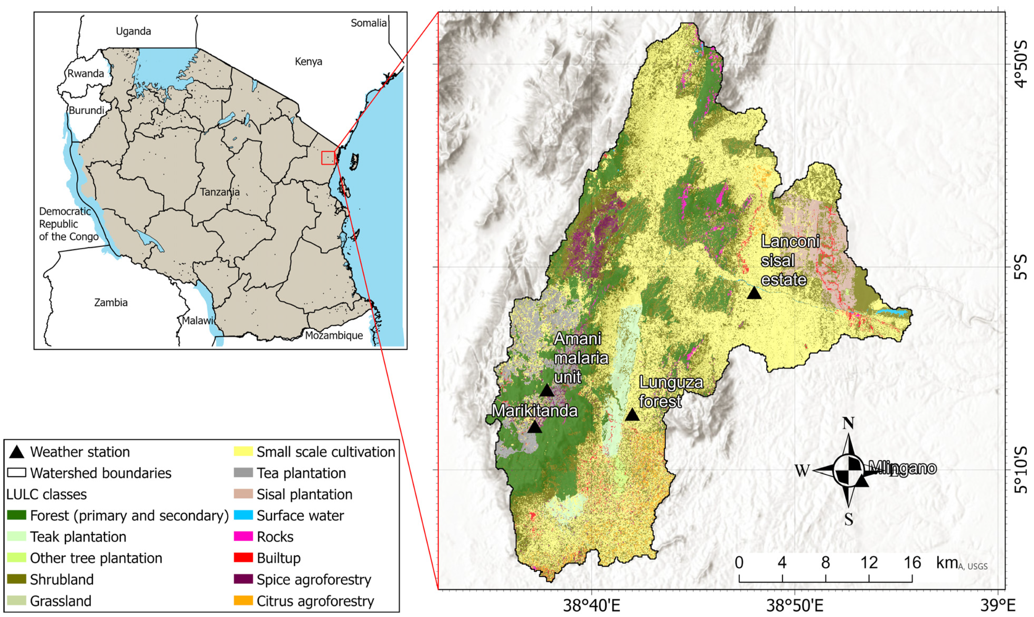
Figure 1. An overview map of the Sigi River watershed, illustrating its geographical extent and boundaries. The map is based on the 2022 land use/land cover classification derived from Landsat imagery [25], overlaid with contour lines to represent topography.
Hydrology 13 00124 g001
Figure 2. An overview of distribution of the 36 soil profiles taken from [29,34,35]. Topographic hillshade from ESRI, NASA NGA, and USGS.
Hydrology 13 00124 g002
Figure 3. Workflow for SWAT model setup and simulation using two soil datasets (SoLIM and SoilGrids), highlighting key steps in watershed delineation, model setup, calibration, and output analysis. Numbers 1, 2, and 3 indicate the sequential steps in the process.
Hydrology 13 00124 g003
Figure 4. Spatial distribution of the six soil units produced by the SoLIM model for the Sigi River watershed.
Hydrology 13 00124 g004
Figure 5. Spatial distribution of soil units produced by SoilGrids for the Sigi River watershed.
Hydrology 13 00124 g005
Figure 6. Spatial distribution of SoLIM soil map prediction uncertainty across the watershed. Lighter colors indicate lower uncertainty and higher model confidence, while darker red areas represent higher uncertainty.
Hydrology 13 00124 g006
Figure 7. Observed and simulated monthly discharge (m3 s−1) and monthly rainfall (mm) for the Sigi River watershed, measured at the Lanconi gauging station, over the full simulation period (1997–2019). Simulated streamflow was derived from the SWAT model, with daily outputs aggregated to monthly time steps for visualization. Model performance was assessed using objective functions calculated from daily observed discharge measurements, ensuring consistency between evaluation and simulation time scales.
Hydrology 13 00124 g007
Figure 8. Flow duration curves (FDCs) for the Sigi River watershed, comparing simulated streamflow from the SWAT model using the SoilGrids soil map (green line) and the SoLIM soil map (red line) with observed discharge measured at the Lanconi gauging station (black line) to calibration and validation. Discharge is shown on a logarithmic scale and plotted against exceedance probability. Shaded areas represent different flow regimes (high flows, mid-range flows, and low flows).
Hydrology 13 00124 g008
Figure 9. Observed and simulated monthly discharge (m3 s−1) and monthly rainfall (mm) for the Sigi River watershed, measured at the Lanconi gauging station, over the selected calibration and validation periods. Simulated streamflow was derived from the SWAT model after calibration, with daily outputs aggregated to monthly time steps for visualization. Model performance was assessed using objective functions calculated from daily observed discharge measurements, ensuring consistency between evaluation and simulation time scales.
Hydrology 13 00124 g009
Figure 10. Flow duration curves (FDCs) for the Sigi River watershed, comparing simulated streamflow from the SWAT model using the SoilGrids soil map (green–black lines) and the SoLIM soil map (red line) with observed discharge measured at the Lanconi gauging station (green–black lines) during the calibration and validation periods. Discharge is shown on a logarithmic scale and plotted against exceedance probability. Shaded areas represent different flow regimes (high flows, mid-range flows, and low flows).
Hydrology 13 00124 g010
Table 1. Summary of soil profile data used in the study, including sources, number of profiles, depth range, and number of horizons.
StudyNumber of ProfilesDepth Range (cm)Newly Generated Number of Horizons in Each Profile
Ndyeshumba (1995) [34]90–1004
Kirsten (2016) [29]90–1004
ISRIC (2014) [35]180–1004
Table 2. Selected SWAT parameters for sensitivity analysis and calibration.
ParameterMethodDescription
Surface runoffCN2r(relative)Curve number
SURLAGv(replace)Surface runoff lag time
Ground water/baseflowALPHA_BFv(replace)Baseflow alpha factor
GW_DELAYa(absolute)Ground water delay
RCHRG_DPv(replace)Deep aquifer percolation fraction
REVAPMNv(replace)Threshold depth of water in the shallow aquifer for “revap” to occur
GW_REVAPv(replace)Ground water revap coefficient
GWQMNv(replace)Threshold depth of water in the shallow aquifer required for return flow to occur
Lateral flowLAT_TTIMEv(replace)Lateral flow travel time
HRU_SLPr(relative)Average slope steepness
ChannelOV_Nr(relative)Manning’s value for overland flow
SLSUBBSNr(relative)Average slope length
CH_N2v(replace)Manning’s n value for the main channel
CH_K2v(replace)Effective hydraulic conductivity in main channel alluvium
SoilESCOv(replace)Soil evaporation compensation factor
SOL_Kr(relative)Saturated hydraulic conductivity of the soil layer
SOL_BDr(relative)Soil bulk density
SOL_AWCr(relative)Available water capacity of the soil layer
Table 3. Key soil physical properties derived from the SoLIM model for the six different soil units obtained (A–F) across the four depth intervals (0–25 cm, 25–50 cm, 50–75 cm, and 75–100 cm). Parameters include bulk density (BD), available water capacity (AWC), saturated hydraulic conductivity (K), carbon content (SOC), and particle size distribution (sand, silt, clay). The respective areas of each soil unit are expressed as percentages of the total watershed area.
Soil Unit
(% of Area)
Depth (cm)BD (g/cm3)AWC (cm3/cm3)K (mm/h)SOC (%)Sand (%)Silt (%) Clay (%)
A
(20%)
0–251.050.20192.02144145
25 501.180.1860.90123850
50–751.220.3460.70133651
75–1001.210.31100.70133453
B
(18%)
0–251.030.19112.00163450
25–501.090.2531.21142462
50–751.210.25210.52122266
75–1001.200.35170.51102268
C
(19%)
0–251.250.22151.50255520
25–501.280.20121.30275122
50–751.300.18101.20284923
75–1001.330.1681.10304624
D
(21%)
0–251.160.101.211.42145234
25–501.180.11411.11164440
50–751.200.1760.98164440
75–1001.270.17100.55104446
E
(10%)
0–251.070.1320.323.16127414
25–501.370.237.190.56107218
50–751.400.1360.34146224
75–1001.360.14280.29124840
F
(12%)
0–251.170.10601.10751510
25–501.260.09550.6078148
50–751.310.08700.4080128
75–1001.330.07500.3082108
Table 4. Soil physical properties from SoilGrids for Acrisols, Ferralsols, and Cambisols across four depth intervals (0–25 cm, 25–50 cm, 50–75 cm, and 75–100 cm). Parameters include bulk density (BD), available water capacity (AWC), saturated hydraulic conductivity (K), carbon content (SOC), and particle size distribution (sand, silt, clay). The respective areas of each soil unit are expressed as percentages of the total watershed area.
Soil Unit
(% of Area)
Depth (cm)BD (g/cm3)AWC (cm3/cm3)K (mm/h)SOC (%)Sand (%)Silt (%)Clay (%)
Acrisol
(64%)
0–251.350.18101.20303040
25–501.400.1760.70322642
50–751.450.1650.50342343
75–1001.480.1550.30352045
Ferralsol
(26%)
0–251.300.2081.00252055
25–501.350.1860.60251758
50–751.380.1740.40261460
75–1001.420.1630.30261262
Cambisol
(10%)
0–251.320.21121.00403525
25–501.360.1990.70423028
50–751.400.1870.50452530
75–1001.450.1660.40462232
Table 5. SWAT-calibrated parameters and their sensitivities for the Sigi River watershed (r = relative change; v = replace value; *** p < 0.001; ** p < 0.01).
ParameterMethodFitted Value (SoilGrid)Fitted Value (SoLIM)t-Stat (SoilGrid)t-Stat (SoLIM)Significance
CN2.mgtr41.1838.42−33.76−45.96***
CH_N2.rtev0.1710.0466.017.48***
SOL_K.solr1911.11−5−6.67***
SOL_AWC.solr0.790.354.51−5.02***
ESCO.hruv0.260.04−3.75−4.02**/***
Table 6. Comparison of annual average water balance components (mm) simulated with the SWAT model using the SoLIM and SoilGrids soil datasets for the Sigi River watershed over the 1997–2019 simulation period.
Water Flow (in mm)SoilGridSoLIM
Precipitation13001300
Water Yield (Discharge)669793
Surface Runoff (SURF Q)474263
Baseflow (LAT Q)60181
Evapotranspiration (ET)642418
Percolation135349
Disclaimer/Publisher’s Note: The statements, opinions and data contained in all publications are solely those of the individual author(s) and contributor(s) and not of MDPI and/or the editor(s). MDPI and/or the editor(s) disclaim responsibility for any injury to people or property resulting from any ideas, methods, instructions or products referred to in the content.