The Observed Wind-Induced Deviation of Drop Fall Trajectories Above an Optical Disdrometer

Abstract

The impact of wind on disdrometer measurements has not yet been demonstrated through controlled reproducible physical experiments. This study aims to provide quantitative evidence of the deviation in raindrop trajectories approaching the sensing area of an optical disdrometer (the Thies Clima LPM) when immersed in a wind flow with a known velocity and direction relative to the sensor orientation. To this end, water drops with diameters between 0.9 mm and 1 mm were released in a wind tunnel and directed towards the instrument’s sensing area. Their trajectories were measured using a high-speed camera and compared with those expected in undisturbed conditions, as well as with the airflow field around the instrument body as measured in previous studies. This experiment provided the first direct measurement of the deviation in individual drop trajectories induced by wind near the Thies Clima LPM, a disdrometer commonly used in hydrological studies and applications. The effect of the non-radially symmetric geometry of the instrument on wind direction was observed, identifying the configuration most affected (parallel to the laser beam). The repeatability of the drop releasing system was checked by releasing multiple drops from the same position. This allowed attributing differences in the observed trajectories to a variation in the drop diameter. The collected dataset can be used to validate numerical models of the wind-induced bias of disdrometers and to develop adjustment functions for field measurements.

1. Introduction

Disdrometers are non-catching type precipitation gauges (NCGs) widely used as a ground reference for developing or validating precipitation retrieval algorithms for weather radars, satellite borne and opportunistic sensors. Estimates of aerial precipitation allow hydrological and hydrodynamic models to be run for the quantification of water balances at catchment scale, as well as for the assessment of fluvial and pluvial flooding issues. When compared with traditional rain gauge measurements, the precipitation rate provided by disdrometers exhibits significant discrepancies (see, for example [1]), meaning that the accuracy of disdrometer measurements must be properly quantified.

Although the impact of wind on traditional precipitation measurements obtained using catching-type rain gauges (CGs) is well understood [2], and adjustment functions have been developed and applied in studies about liquid and solid precipitation (see, e.g., [3,4]), this issue is rarely addressed in the literature when it comes to measuring microphysical and integral precipitation properties using disdrometers [5]. Due to the complex shape of the disdrometer, which produces an obstruction to the trajectories of incoming hydrometeors and is highly dependent on wind direction, the wind-induced bias of such measurements can be even larger than for CGs. Moreover, the recent literature has explicitly linked the magnitude of wind-induced bias for CGs to the microphysical properties of precipitation (see, e.g., [6]). This means that measurement biases for NCGs affect the accuracy of CG measurements and propagate through hydrological modeling chains that use traditional rain gauge measurements as input data.

Various studies have noted that disdrometer measurements in windy conditions may differ from those of other reference instruments, and the instrument performs differently when exposed to wind from different directions (see, e.g., [7]).

Strong winds are typically associated with tropical cyclones, for example. Lin et al. [8] investigated possible sources of bias in precipitation measurements using an optical disdrometer (the OTT Parsivel) in such conditions, based on data collected simultaneously by a disdrometer and an automatic weather station on board a mobile observation vehicle. Measurements were taken during four typhoons in China between 2014 and 2018. The rainfall intensity obtained from the disdrometer was found to be lower than that obtained from the weather station, with the underestimation increasing with the wind speed. An empirical wind-adjusted quality control method was therefore proposed.

Previously, Friedrich et al. [9] investigated the impact of the wind speed and direction on optical disdrometer measurements. This was prompted by the observation of artefacts in the distribution of particle sizes when an unexpected concentration of large-diameter raindrops with unrealistic fall velocities (far from the terminal velocity and which do not follow the equation of motion for an object in free fall) was recorded using OTT Parsivel disdrometers in strong winds during a dedicated experiment. This effect was associated with stationary disdrometers but not with articulating ones (which automatically rotate their sampling area into the wind), thus highlighting the impact of wind direction.

The impact of wind on raw velocity–diameter spectrographs obtained from the Thies Clima Laser Precipitation Monitor (LPM) optical disdrometer was experimentally measured by Capozzi et al. [10], who noted a progressive increase in the wrongly allocated hydrometeors in the particle size and velocity distribution (PSVD) matrix up to 70% at wind speed higher than 8 m s⁻¹.

The signature of wind-induced bias on disdrometer measurements therefore emerges from the literature, but direct evidence has not yet been provided. However, previous studies have already examined this phenomenon in the context of CGs, which only provide integral measurements of the precipitation process. Evidence of wind-induced bias has been sought for many years using wind tunnel (WT) experiments; though in many cases, the studies were limited to visual or barely quantifiable results (see [11,12,13,14,15,16]).

These experiments began with the early work of Bastamoff and Witkiewitch [11], although Jevons [12] initially used a simple WT test involving smoke trails from smoldering brown paper to support his pioneering explanation of the wind exposure problem (also called the Jevon’s effect after [17]). Sanuki et al. [13] conducted tests in the WT to optimize two types of wind shield for rain gauges (conical and hollow ring-shaped designs), visualizing the flow deformation around the instrument funnel and windshield by tying wool strings to the model and taking pictures in the WT. The aim of the assessment of the windshield design was to minimize eddies in the airflow field.

Robinson and Rodda [14] also studied the airflow pattern around four types of CGs in the WT, using tuft indicators and smoke trajectories to visualize the aerodynamic behavior of two rain gauges with cylindrical shapes, a drop counter gauge, and a champagne glass-shaped gauge.

Warnik [15] first visualized the deviation of hydrometeor trajectories when traveling across the disturbed airflow zone close to the gauge collector by injecting real and sawdust snow into the WT to study the quantitative catch of the model gauge. Later, Green and Helliwell [16] measured the trajectories of injected water drops above a cylindrical CG using photographs taken with a reflex camera but with low detail.

More recently, Cauteruccio et al. [18] performed a detailed fully quantitative experiment addressing various CGs with different (though always radially symmetric) external geometry in dedicated WT tests, using a high-speed camera and particle image velocimetry. The results showed that the typical shapes of traditional tipping-bucket and weighing rain gauges (cylindrical and ‘chimney’) perform less well in windy conditions, while an inverted conical shape is less susceptible to wind impact.

However, to the authors’ knowledge, no similar studies exist for disdrometers or non-catching precipitation measurement instruments in general. The fact that disdrometers typically have a more complex non-radially symmetric geometry due to the measurement principle involved adds to the complexity of the problem.

In this study, a WT experiment was conducted to provide quantitative evidence of the deviation in raindrop trajectories in proximity to the sensing area of the Thies Clima LPM optical disdrometer, when immersed in a wind field with known velocity and direction relative to the sensor orientation. The trajectories observed were measured using a high-speed camera and compared with each other and with those in the least disturbed conditions, as well as with the airflow field around the instrument body, as measured in previous studies. This experiment provides the first direct measurements of the wind-induced bias of individual drop trajectories for a commonly used disdrometer in hydrological studies and applications.

The collected dataset enables numerical models used to quantify the wind-induced bias affecting NCG measurements to be validated. Numerical modeling allows a wide range of combinations of wind speed, wind direction and drop size to be investigated, extending beyond the limits tested in the wind tunnel. Continuous adjustment functions can be derived and applied a-posteriori or in real time when contemporary disdrometer and wind measurements are available. Drop size distribution measurements propagate in the adjustment of traditional CG measurements when wind is present, and therefore in the associated hydrological applications. The parameter values of hydrological and hydrodynamic models can vary significantly depending on whether corrected or uncorrected precipitation time series are used.

The paper is organized as follows: Section 2 describes the disdrometer used in the tests and provides technical details of the experimental setup, including the drop-releasing device and WT equipment. It also presents the drop detection system, along with the post-processing method used to retrieve the trajectories of the released drops from high-speed footage, as well as their deviation close to the instrument body. Section 3 presents experimental results, highlighting the observed aerodynamic effects in the measured drop trajectories. The repeatability of the experiment is demonstrated, and a comparison is provided between sample trajectories and the least disturbed ones. Finally, Section 4 discusses the main results in terms of their application and use in further research, providing concluding remarks.

2. Materials and Methods

2.1. The Thies LPM Disdrometer and Previous WT Experiments

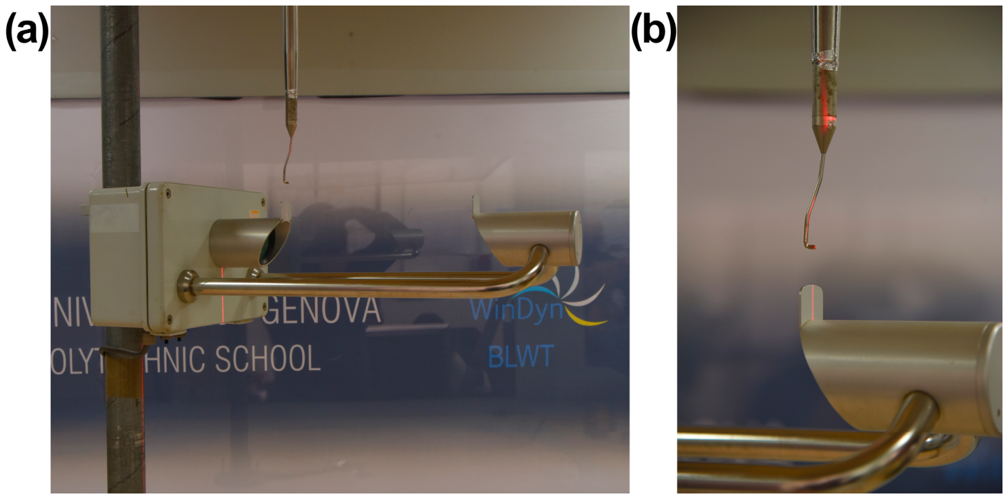
The Laser Precipitation Monitor (LPM) is a commonly used optical transmission disdrometer manufactured by Thies CLIMA, Adolf Thies GmbH & Co. KG, Göttingen, Germany ([19], see Figure 1a). The instrument’s transmitting head is directly attached to the circuitry box, while the receiver head is connected to it via supporting arms. The emitter head uses a laser diode to produce a 20 mm-wide light beam, which is detected by a horizontally aligned receiving sensor.

A photodiode in the receiver head converts the power of the laser beam into an electrical signal, which is reduced by light blockage due to hydrometeors crossing the beam. Power reduction is proportional to the size of the falling hydrometeor, and the fall velocity is obtained from the duration of the beam blockage (extinction). The combination of hydrometeor size and fall velocity enables other objects that may cross the laser beam, such as insects, to be excluded. In such cases, in fact, the size–velocity relationship would differ from that expected for hydrometeors (e.g., as described by Gunn and Kinzer [20]). The laser diode operates at a high frequency (173 kHz), and a low-pass filter is used in the receiver to minimize interference from ambient light.

The diameter of liquid hydrometeors is categorized into 22 classes ranging from 0.125 to ≥8 mm, while the fall velocity is categorized into 20 classes spanning a range of 0.2 to ≥10 m/s. The distribution of the hydrometeor size and fall velocity over class binning, aggregated at one-minute resolution, is also used to calculate the precipitation intensity and amount, visibility, the kinetic energy of precipitation, and the radar reflectivity.

A single user-configurable data telegram is reported at a fixed interval, which is typically set to one minute. The typical output telegram provides information on the particle size and velocity distribution, but raw measurements can also be included. For each hydrometeor detected, the raw telegram provides size (diameter) and fall velocity information. However, the two telegrams cannot be output at the same time.

Following a comparison with an unspecified reference sensor at a wind speed of less than 3 m/s, the manufacturer states that the margin of error in the measurement of the precipitation intensity (rain equivalent) is ≤15% for rainfall at an intensity of up to 20 mm/h and ≤30% for snow [19]. The same installation instructions provide specific guidance on how to orient the disdrometer onsite. In the Northern Hemisphere, the laser beam should be oriented towards the south (±10°). The receiver should be positioned on the south side to minimize the impact of sunlight on the sensor. However, no guidance is provided regarding the possible impact of wind, which can affect the trajectories of approaching hydrometeors, modifying the number of drops that reach the instrument’s sensing area and the expected combinations of drop size and fall velocity.

Figure 1a illustrates the instrument’s non-radial symmetry. While the body of the instrument is symmetrical with respect to a vertical plane passing through the longitudinal axis of the sensing area (i.e., the laser beam), there is no symmetrical surface perpendicular to the laser beam. This demonstrates that the angle at which the wind impacts the instrument can have a significant effect, as the instrument presents different cross-sectional areas to the wind depending on its direction.

A comprehensive measurement campaign had previously been performed by Chinchella et al. [21] in the WT of the University of Genoa (Italy) to characterize airflow velocity components near the surface of the Thies Clima LPM. This WT is composed of a closed-loop subsonic circuit and is used for aerodynamic and civil engineering experiments. The WT has a working section with a total length of 8.8 m and a cross-sectional area of 1.7 × 1.35 m² (width × height). Airflow measurements were taken at the end of the working section where the naturally developed wall boundary layer is 0.13 m thick. A static Pitot tube was placed at the top of the test section to measure the reference wind speed. Local wind speed measurements were taken using a fast-response four-hole ‘Cobra’ probe mounted on a traversing system with three degrees of freedom (see [22] for additional details). A full-scale Thies LPM instrument was installed on a supporting pole within the WT and fixed to a rotating base plate. A laser beam was used to check the alignment between the instrument’s longitudinal axis and the Cobra probe’s head, which was fixed to a traversing system (see Figure 1b). This process was repeated for nine wind directions by rotating the instrument on its supporting pole. Measurements showed that significant disturbance develops close to the instrument body, which affects its measuring area and strongly depends on wind direction.

2.2. The Experimental Setup

To measure the effect of the aerodynamic disturbance on the trajectories of hydrometeors, a new experimental campaign was carried out using the large-scale WT facility of the Politecnico di Milano (Italy). This experiment was conducted as part of the Italian national PRIN 2022MYTKP4 project, “Fostering innovation in precipitation measurements: from drop size to hydrological and climatic scales”.

A dedicated experimental setup was prepared in the WT, complete with a full-scale instrument. The WT facility features a low turbulence high-speed chamber, where the instrument under test and the drop generation and release systems were installed. The chamber (4 m wide, 3.8 m high and 6 m long) is characterized by a nearly laminar flow (i.e., the along-wind turbulence intensity is lower than 0.2%) and a boundary layer extending approximately 0.1 m from the walls. The instrument was fixed to the floor of the test chamber, centered in the along-wind direction.

Water drops were released into the airflow field, and their deviated trajectories close to the instrument’s sensing area (where the airflow field is modified by the presence of the instrument body) were captured with a high-speed camera. Various combinations of wind direction and drop release height were tested in a controlled environment by rotating the instrument in the WT.

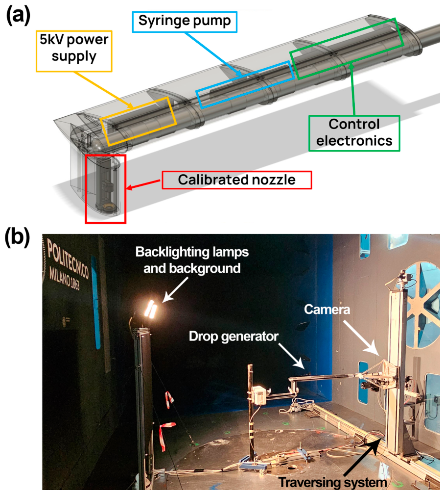
A purpose-built drop generator was used to release drops into the airflow on demand. The apparatus comprises a control unit, a syringe pump and an electrostatic release system (see Figure 2a). Once a drop of the desired volume is produced by the syringe pump and formed at the tip of a calibrated needle, its detachment is achieved by applying a 5 kV potential difference between the needle and a metallic ring positioned few millimeters below. This improves the reproducibility of the drop volume by limiting the effect of surface tension during detachment. The entire drop releasing system is covered by an aerodynamic outer shell that was modeled as a NACA symmetric airfoil [23] and 3D printed, to minimize flow disturbance.

To precisely adjust the release position of the water drops, the generator was mounted on an automated traversing system, allowing movement in the longitudinal and vertical directions. Considering the transversal direction, the generator is positioned so that the drop would be released precisely in the middle of the WT chamber where the center of the disdrometer laser beam is also positioned. A similar drop generator was developed and extensively tested in a fixed laboratory assembly during a previous project and was then used to calibrate disdrometers in static airflow conditions [24]. Furthermore, for the aerodynamic drop generator, preliminary tests were carried out in the WT of the University of Genoa to check that the drop detached smoothly and to identify any possible deviations in its trajectory that could result from the generator assembly.

The trajectory of each released drop was recorded close to the instrument body on the along-wind vertical plane by using an i-SPEED 220 high-speed camera (PTC International Ltd, Hong Kong), with a resolution of 1600 by 700 pixels. The camera was equipped with a Fujinon CF35HA lens and was positioned 1.7 m from the center of the WT, with a framerate set to 1000 fps. A black background was also inserted in the WT, and lamps were used to illuminate the released drops from behind. This was necessary to ensure a high contrast level in the recordings and facilitate automated image post-processing. To appreciate the deformation of the drop trajectories when the flow field is disturbed by the presence of the instrument body sufficiently strong wind is necessary. Experiments were therefore conducted at a wind speed of 10 m/s with generated drop diameters between 0.9 mm and 1 mm, which were released from different heights above the instrument’s sensing area. Three different wind directions were tested: 0°, 45° and 90°, obtained by physically rotating the instrument inside the WT. The repeatability of the drop-releasing system was checked by releasing five drops in each direction at a fixed releasing height. The configuration of the test chamber of the WT is shown in Figure 2b.

2.3. Processing of Drop Trajectories

The camera was synchronized with the drop generator and recorded a 0.3 s video for each drop released, capturing about 300 frames. This time window was sufficient for the drop to detach from the generator, accelerate through the air and reach the instrument with about 50 ms to spare.

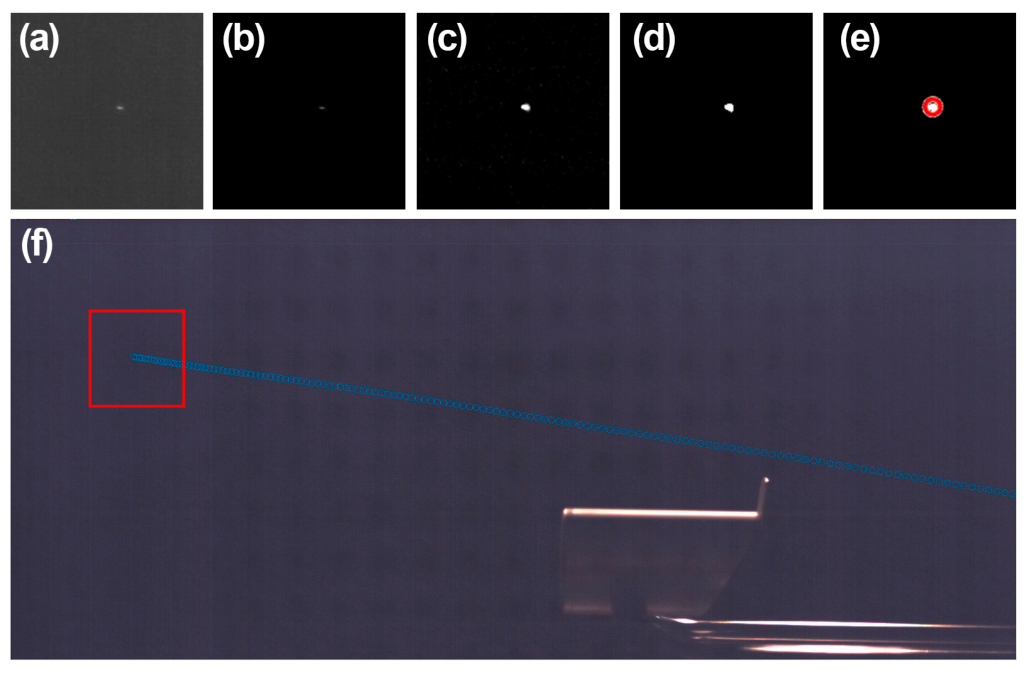
Figure 3 shows the post-processing steps applied to the sub-frame of a sample drop position and the retrieved trajectory. To retrieve the drop trajectory, each frame was converted to greyscale (Figure 3a). The background was then removed, and the effect of digital noise was reduced by subtracting the average of the first eight frames, in which the drop was not yet visible, from the subsequent frames (Figure 3b). Finally, a combination of Gaussian and Laplacian filters was applied to enhance the drop contours (Figure 3c). Once binarized (Figure 3d), the positions of the white pixels were detected automatically (Figure 3e). To eliminate any pixels produced by residual digital noise or reflections, the instrument body was masked using a black frame. Finally, isolated pixels and pixels that did not move between frames were also removed.

After each frame was thoroughly cleaned, the outline and center of the drop were detected, enabling the entire trajectory to be reconstructed (see Figure 3f). Conversion of the trajectories’ coordinates from the image reference system to the WT reference system is possible, as the position of the camera and focal length of the lens used are known. Furthermore, the drop velocity in the 2-D shooting plane was calculated, since the time interval between two subsequent images is known (1 ms).

The recorded drop trajectories provide evidence of the particle–fluid interaction that is responsible for their significant deviation close to the instrument body. The drop generator was positioned 0.5 meters upstream of the center of the instrument’s sensing area, with its elevation changing from a maximum coordinate of Z = 0.16 meters above it to a minimum of Z = 0.08 meters. For ease of referencing the drop release position in the following figures, the release elevation will be indicated with the relative vertical coordinate H, considering H = 0 as corresponding to the highest drop release elevation (Z = 0.16 m).

To visualize the aerodynamic disturbance experienced by the drops in flight, numerical simulation results from the work of Chinchella et al. [21] were also used. We calculated the successive positions of the drop along each trajectory with respect to the airflow velocity field numerically simulated in that study. Then, we extracted the airflow velocity components along the path of each drop released, as presented in the following.

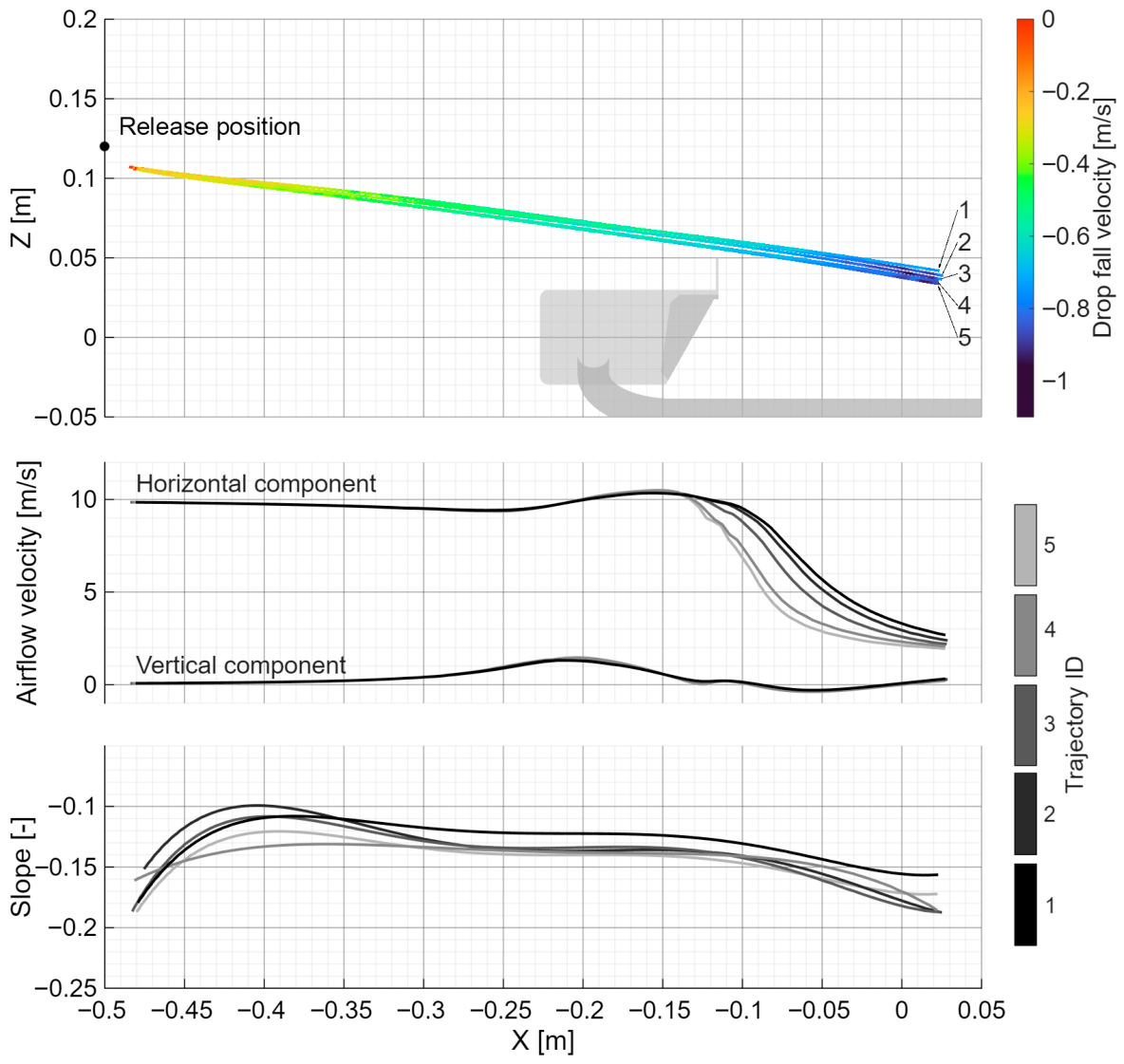
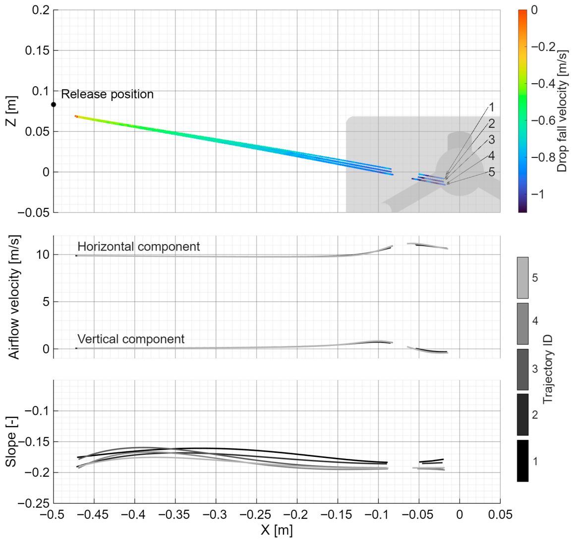
To investigate the impact of the aerodynamic disturbances produced by the instrument on the drop trajectories, a series of five drops were released at H = 0, −10, −20, −30 and −35 mm. This test was repeated for each wind direction, with the results presented in Figure 4, Figure 5 and Figure 6 for 0°, 45° and 90°, respectively.

3. Results

3.1. Aerodynamic Effect on Drop Trajectories

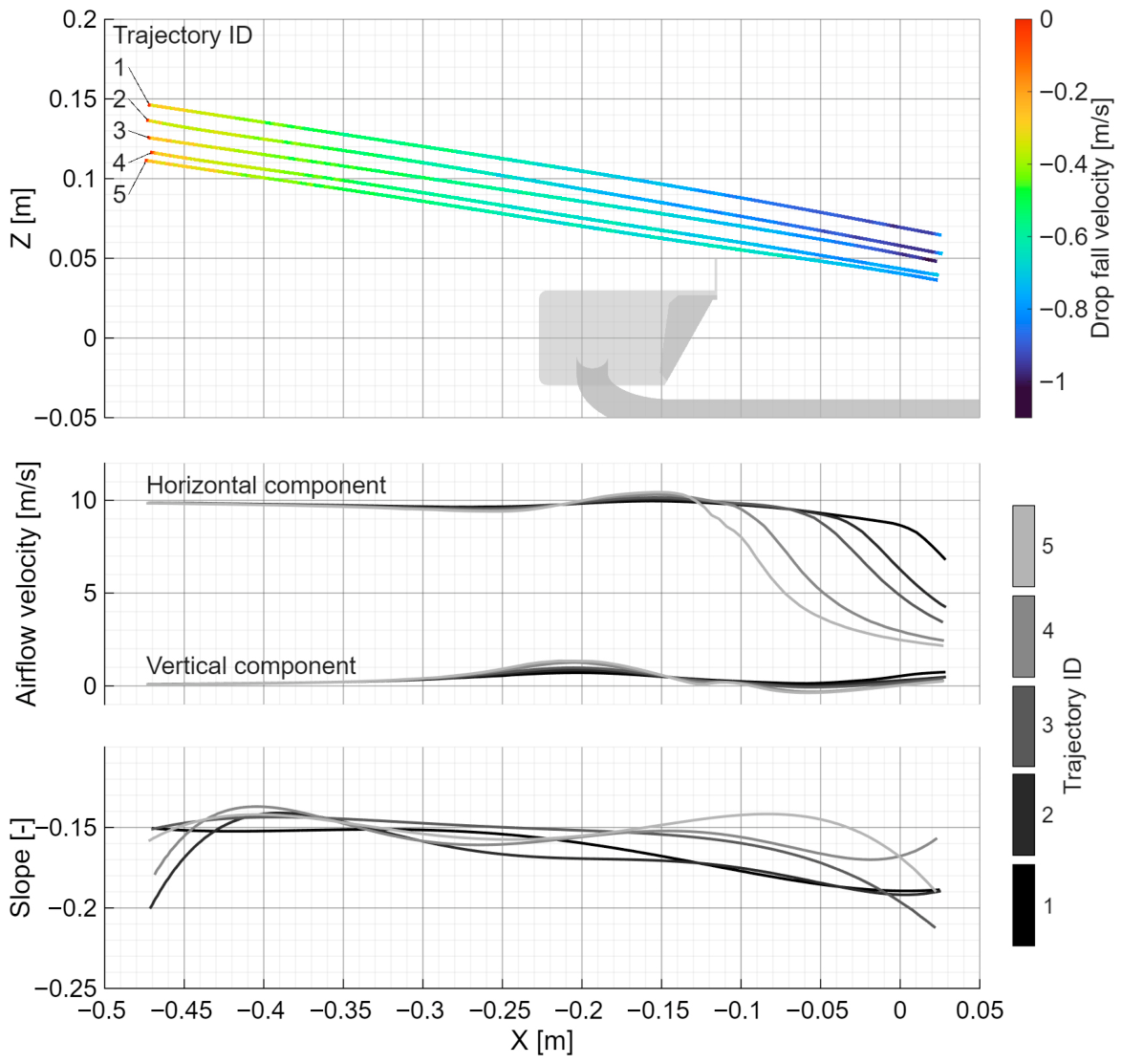
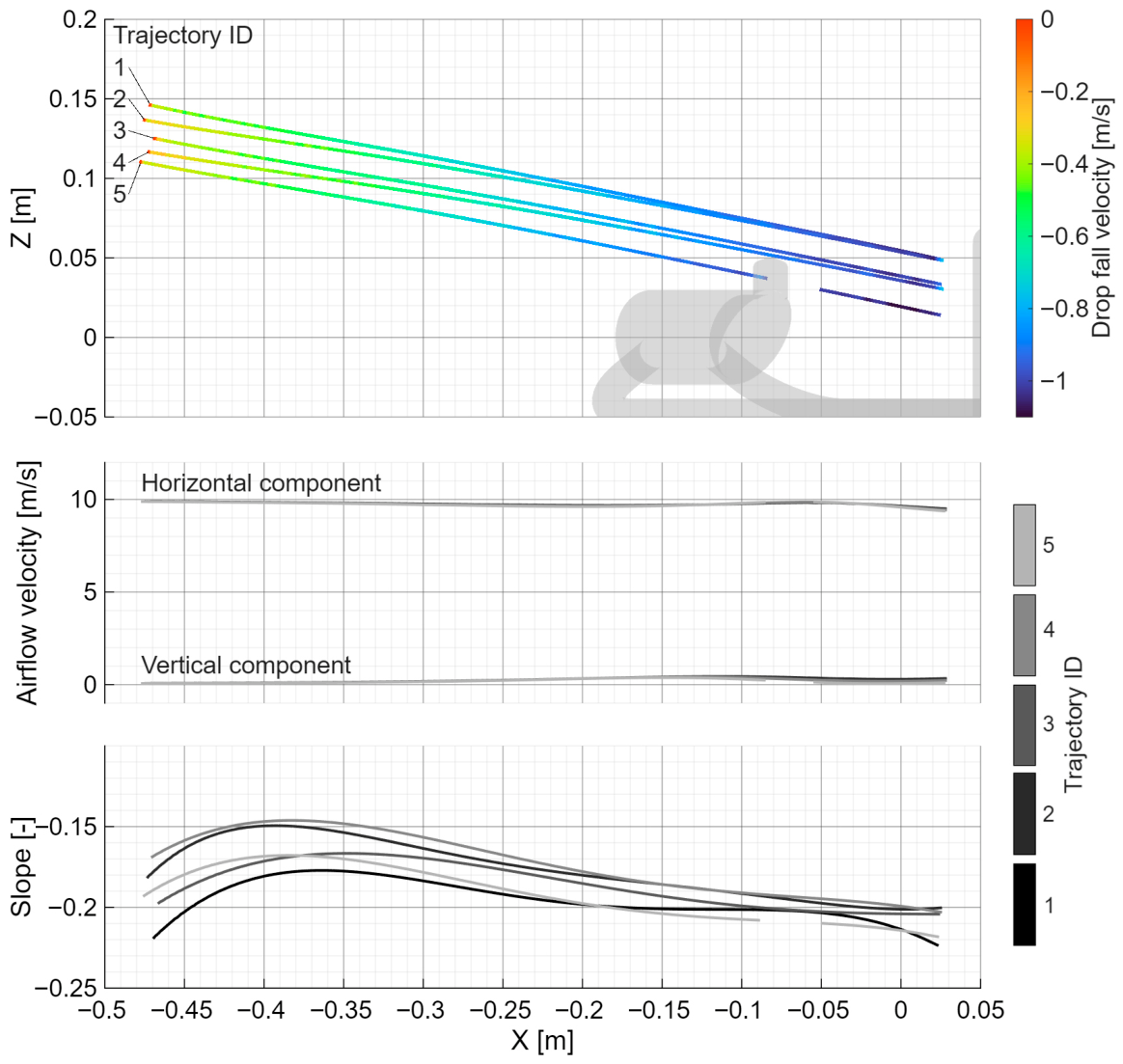
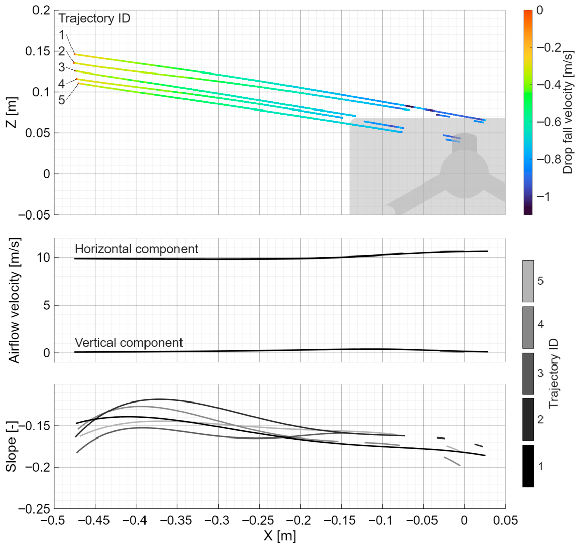
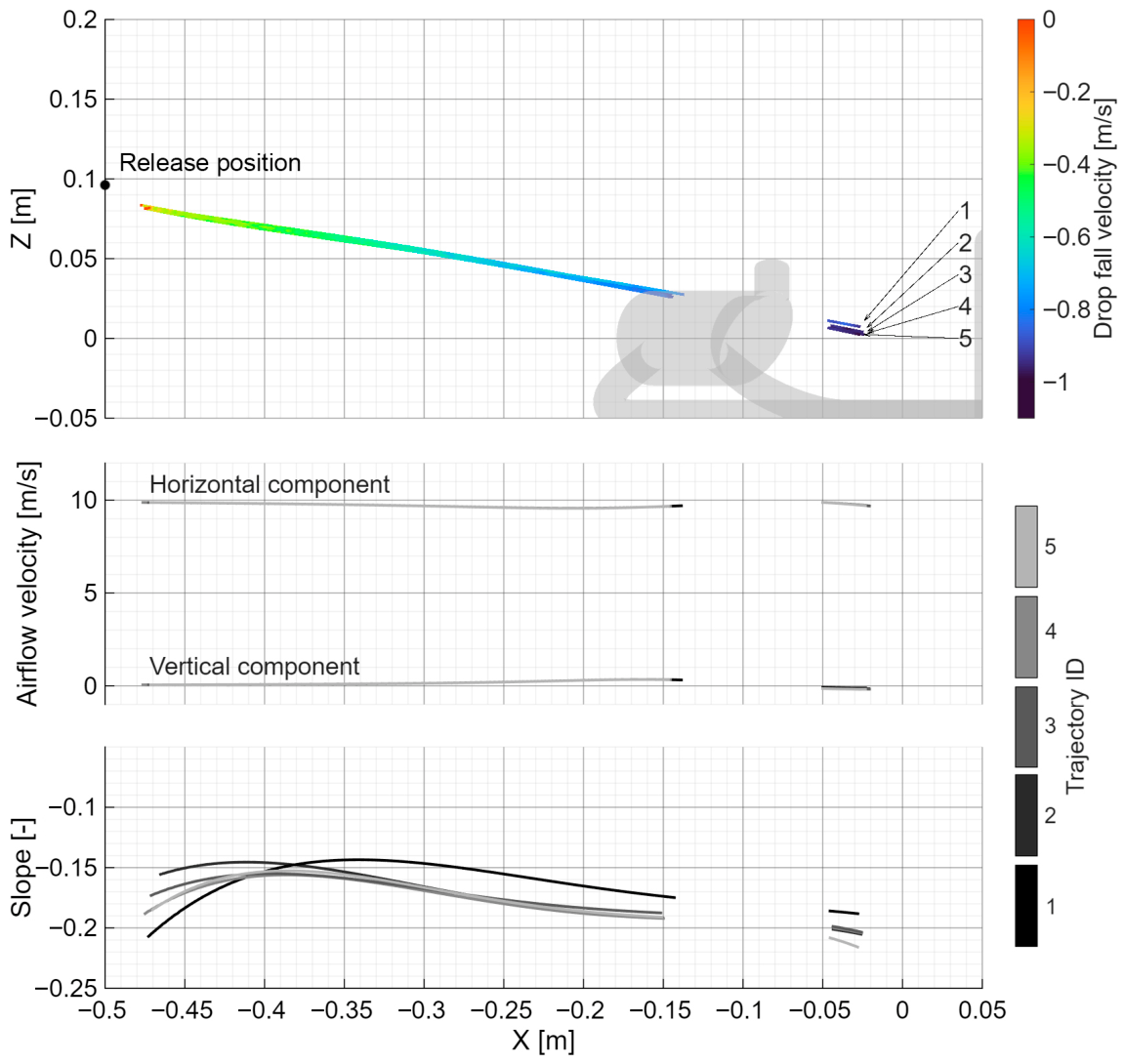
In the figures below, the drop trajectories are depicted in the top panel and are color-coded according to their measured fall velocity (the vertical component of the drop velocity), highlighting the vertical acceleration experienced by the drop after detachment and its dependence on aerodynamic disturbance as it approaches the instrument. The central panel illustrates the numerical airflow velocity components along the drop trajectory obtained from numerical simulation. The bottom panel shows the measured slope of each trajectory, calculated using a central difference scheme to smooth the results.

The top panel of Figure 4 shows that the five trajectories start almost parallel to each other and are then diverted to a different extent when approaching the instrument. Beyond a horizontal coordinate of about X = −0.25 m, drops starting from a lower elevation show a reduced vertical velocity than those starting from a higher elevation. This is consistent with the onset of a strong updraft (>1 m/s) along the trajectories as shown in the central panel. As expected, this updraft is higher for trajectories that are closer to the instrument body and mostly concentrated above the first half of the receiver’s head.

Along the remaining path, updraft is mostly absent, while a consequent abrupt reduction in the horizontal airflow velocity component appears. This reduction is due to the boundary layer and the flow separation produced by the thin metallic plate protruding from the receiver head. Drops released from a lower elevation decelerate first and show significant diversion. This reflects into a change of slope in the trajectory, as observed in the bottom panel. Overall, a clear effect of the obstruction due to the instrument body and its small geometric features is observed, with a non negligeable impact on the drop trajectories.

The trajectories obtained for a wind direction of 45° are shown in the top panel of Figure 5. In this and in the following graphs, the trajectories may be partially incomplete because they are hidden behind the instrument body for a portion of their path. In the top panel, differences are evident between drops having an ID of 1, 3 and 5 and drops having an ID of 2 and 4. Trajectories are almost parallel for their entire path if compared within the same group, but the two groups differ significantly.

This is notwithstanding the fact that both the horizontal and vertical components of the airflow velocity are almost identical for all trajectories, as shown in the central panel. Therefore, the difference can only be ascribed to the different diameter of the drops as released by the drop generator. This aspect of repeatability is investigated in the following subsection.

Considering each group separately, it is evident that no significant aerodynamic disturbance is present along the observed trajectories. This is also evident in the bottom panel, where the slope of the trajectories is presented. In all cases, indeed, the slope gradually decreases, while drops tend to reach their terminal velocity.

Finally, Figure 6 presents the results obtained for a wind direction of 90°. Similarly to the previous case, the trajectory with ID = 2 and 4 shows a different behavior than the other ones. The central panel also shows that the horizontal and vertical components of the airflow velocity are slightly more disturbed than in the previous case.

Some limited updraft occurs above the upwind supporting arm, while some limited acceleration is evident just after encountering the instrument’s main body. Considering the slope of the observed trajectories, similar to the behavior observed in Figure 5, a gradual decrease in the slope while drops approach their terminal velocity is evident.

3.2. Repeatability

To evaluate the repeatability of the drop releasing system, tests were also conducted by releasing multiple drops from the same height. This is important since some differences in the trajectories were noted that can only be explained with a change in the drop diameter. During these tests, the release height was adjusted so that the drop would reach the instrument sensing area and could be measured by the instrument. During the tests, however, for a wind direction of 0°, drops could not reach the instrument sensing area. Meanwhile, a few measured drops are available for tests at a wind direction of 45° and 90°.

After accounting for the instrumental error of this specific disdrometer, as reported in the work of Chinchella et al. [24], the measured drop diameter ranged between 0.8 mm and 1.1 mm, with most of the diameters being between 0.9 and 1 mm. This variability may explain some of the discrepancies shown in the previous images.

The trajectories used for evaluating repeatability are presented in Figure 7, Figure 8 and Figure 9. The top panel of Figure 7 shows good agreement between the trajectories of five drops released from the same position, at H = −40 mm. Both the overall path and the fall velocity gradient are very similar for all the observed trajectories in this group, with a limited dispersion in their terminal portion.

However, it also highlights the strong nonlinearity of the problem. As shown in the central panel, small differences in the trajectories result in the drop crossing the separation layer significantly earlier or later, which induce larger or smaller deviations in the last portion. The overall spread of the terminal position of the trajectories is about 10 mm.

In terms of slope, the behavior is quite consistent, as shown in the bottom panel. While the slope still increases overall, like in previous cases, an abrupt change is evident at about X = −0.1 m, due to the crossing of the separation layer, after which drops enter a low flow velocity zone.

At a wind direction of 45°, as previously shown, aerodynamic disturbance is at a minimum. This is also evident in Figure 8 for a fixed release height of H = −64 mm, where the dispersion of trajectories (top panel) is minimal. A different release height was used because, when the instrument is held at different angles to the wind, the starting point must be adjusted to aim at the center of the instrument’s sensing area.

The horizontal and vertical components of the airflow velocity encountered by the drop (central panel) are nearly constant along the entire trajectory. The slope of the trajectories is also similar between all drops, except for the one with ID = 1. Discarding this trajectory, the overall maximum dispersion at the terminal position would be less than 5 mm; otherwise, it remains below 10 mm.

Finally, Figure 9 shows in the top panel five trajectories of drops released at H = −77 mm for a wind direction of 90°. With respect to the previous case, a higher dispersion is evident, which is slightly over 10 mm at the terminal position and is comparable to the case of a wind direction equal to 0°. In the central panel, both the horizontal and vertical airflow velocity components are shown to increase when the drop encounters the instrument supporting arm. In terms of slope, the gradual decrease shown in the previous cases stops when approaching the instrument supporting arm, and the slope of the five trajectories remains almost constant, with even a limited increase.

3.3. Assessment of Drop Deviation

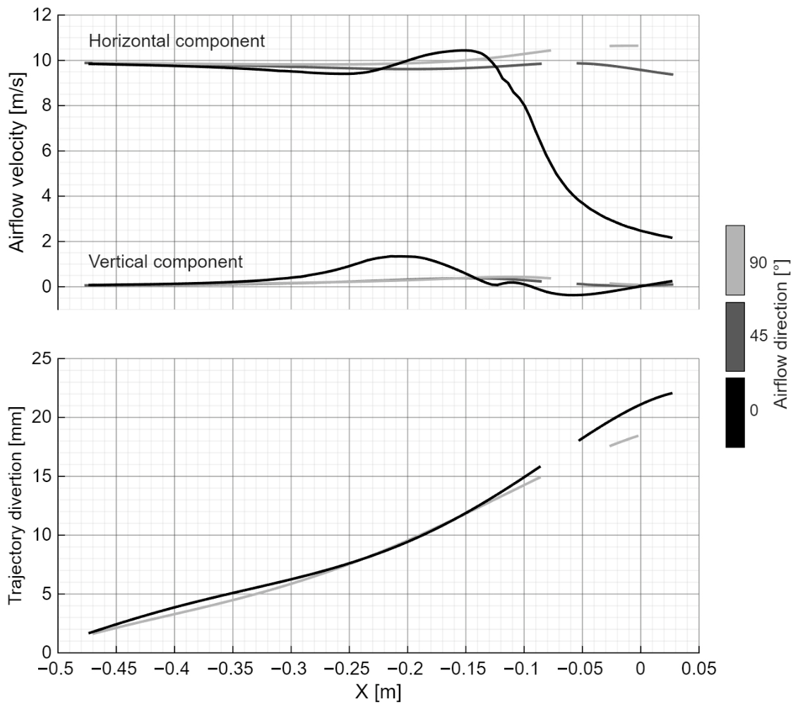
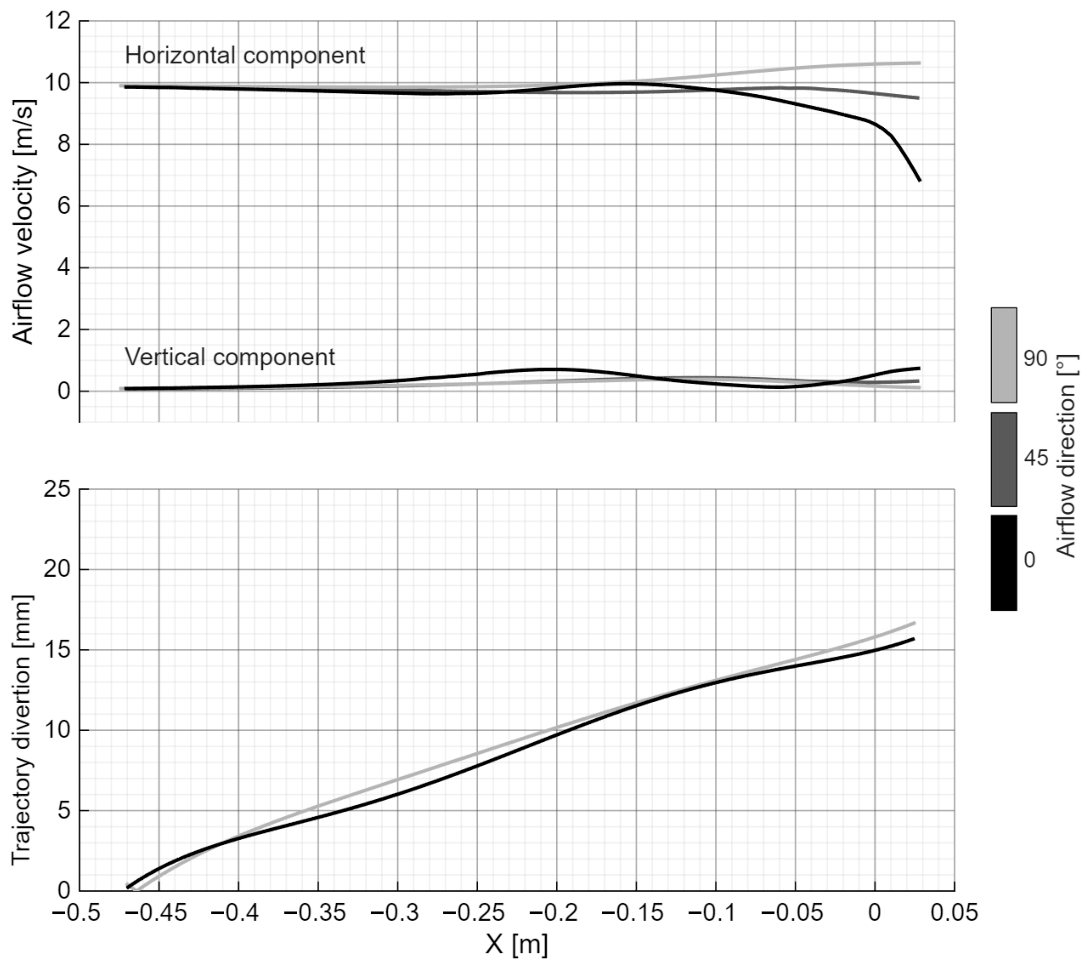
To quantify the influence of the wind direction on the aerodynamic disturbance experienced by the drop trajectories, deviations were calculated for drops released at H = 0 and H = −35 mm for the three investigated wind directions. The diversion of the drop trajectory was obtained as the absolute distance between the observed and reference “undisturbed” trajectory. Among the three trajectories starting from each specific position, this was chosen as the one that encounters the least aerodynamic disturbance during its flight. In both cases, the reference trajectory was the one observed at a wind direction of 45°, where the aerodynamic disturbance is minimal.

The horizontal and vertical components of the airflow velocity along each trajectory of drops released from the same height but for different wind direction are shown in the top panel of Figure 10 and Figure 11, together with the deviation from the least disturbed trajectory (bottom panel).

Figure 10 shows the effect that different wind directions may produce on drop trajectories approaching the instrument from the same release position. As can be seen from the top panel, when drops are released at H = 0, the one observed for a wind direction of 45° encounters the least disturbance. Meanwhile the drops released for a wind direction of 0° encounter first some strong updraft, followed by a reduction in the horizontal component of the airflow velocity. The drop observed for a wind direction of 90° instead encounters first a limited updraft followed by an increase in the horizontal airflow velocity component. In both cases, the interaction between the airflow and the drops produces a diversion of the two disturbed trajectories that reaches a maximum of about 16 mm as shown in the bottom panel. This is noticeably higher than the maximum dispersion shown in Figure 7, Figure 8 and Figure 9, meaning that this diversion cannot be ascribed to drop size variability alone.

Another example of the diversion of drop trajectories depending on the wind direction is shown in Figure 11. In this case, drops are released at H = −35 mm, closer to the instrument body. Similar considerations to the previous case hold, with the trajectory observed for a wind direction of 45° experiencing again the least disturbance (see top panel). However, the overall flow disturbance in all three cases is significantly higher in this case, especially for a wind direction of 0°. An increased diversion of the trajectories (bottom panel) is obtained, especially for the trajectory observed for wind direction of 0°. In that condition, the increase is about 45% with respect to the results reported in Figure 10, while for a wind direction equal to 90°, the increase is only about 10%.

4. Discussion

This study provides evidence of the deviation in the trajectories of falling drops when they approach the sensing area of the Thies LPM disdrometer in the presence of a wind flow. This is due to the aerodynamic behavior of the instrument’s body and the perturbation it provides against the wind. WT results demonstrate that the deviation in drop trajectories depend not only on the release height and drop diameter but also on the instrument’s orientation relative to the wind direction (angle of attack).

Although this was expected, there has been no quantitative experimental evidence of the wind-induced deviation in drop trajectories for non-catching precipitation measurement instruments (including disdrometers) in the literature. The results of this study enhance our understanding of environmental biases in precipitation measurements by demonstrating how wind can introduce a form of ‘catching’ bias, even in non-catching instruments. Drops that are aerodynamically deflected may swerve away from the sensing area and be entirely missed, or they may cross the sensing area from trajectories that would not be intercepted in the absence of wind.

The overall bias in rainfall measurements is the result of integrating all raindrop trajectories that cross the sensing area within a given period. This depends on the number and size distribution of natural raindrops, as well as the wind speed and direction. While it is difficult to simulate this in a WT, numerical simulation can help calculate the resulting effect on multi-dispersed rain when the instrument is impacted by wind.

The results presented above can be readily used to validate numerical models of the wind-induced bias, which are based on the simulation of raindrop trajectories across the airflow field disturbance caused by the instrument’s bluff-body behavior. These models reproduce the deviation of these trajectories when the drop approaches or crosses the sensing area of the instrument. Due to the significant assumptions involved, computational fluid dynamics simulations and particle tracking algorithms require validation against physical measurements.

In the case of simple radially symmetric geometries like those of traditional catching-type precipitation measurement instruments, validation was successfully obtained by comparing simulations with dedicated WT experiments. However, this has not yet been possible for the more complex geometry of non-catching instruments, including disdrometers, due to a lack of quantitative experimental evidence. The geometry of such instruments comprises various thin protruding elements, such as the vertical shielding plates of the Thies Clima LPM, as well as bluff elements, such as the circuitry box of the same instrument. Therefore, transferring the validation of numerical simulation models obtained for the much simpler catching-type instruments is not straightforward. The results presented in this paper fill this gap and foster improved accuracy in precipitation measurements using disdrometers.