Development of the Boundary Water Level Method: A New Approach for Continuous Flow Monitoring in Open Channels

Abstract

This research develops a new low-cost method for continuous flow monitoring in open channels. Flow is calculated using a standard 1D hydraulic model that integrates surveyed cross-sections and water level measurements at the boundaries of a studied reach, from which the name Boundary Water Level Method (BWLM) is derived. By implementing low-cost ultrasonic sensors for water level measurement, the method gains advantage for application on smaller channels, which are often not included in national hydrological monitoring networks due to limited budgets. New and innovative monitoring methods in hydrology are a necessary alternative to increasing the monitoring budgets, especially for continuous, real-time flow monitoring. Like any novel method, it requires validation under the intended environmental conditions, especially when designed primarily for ungauged channels. Validation was conducted on two test-sites by comparing the BWLM discharge and the discharge from official hydrological stations, with an error of up to 15%. BWLM provides reliable discharges using estimated hydraulic roughness values based on the literature and experience. Sensitivity analysis of the estimated hydraulic roughness coefficient demonstrated a substantial influence on the resulting discharge values. This has to be considered when implementing the method in unstudied basins.

1. Introduction

1.1. Motivation and Problem Statement

Most of the countries worldwide face challenges related to an insufficiently developed hydrological monitoring network and a limited availability of real-time hydrological data. The most important hydrological variables are water level (stage) and discharge (flow). The measurement, collection, and processing of hydrological data require substantial financial resources, as they involve extensive field measurements combined with demanding office-based work. Consequently, budgetary constraints directly affect the quality and coverage of hydrological monitoring systems [1]. One alternative to increasing financial investments is the development of new, more practical and cost-effective measurement methods, which entail lower implementation costs compared to conventional approaches [2,3].

In addition to data availability, the temporal and spatial distribution of measurements, as well as their overall quality, are of critical importance. While hydrological monitoring networks on larger rivers were often established more than a century ago for purposes such as navigation, hydropower exploitation, or flood protection, smaller watercourses frequently remain inadequately monitored.

Effective and responsible management of rivers and water resources requires the establishment of an adequate monitoring network for the systematic collection and analysis of measured data. Hydrological data gains relevance when provided with minimal temporal delay. Furthermore, due to the dynamic nature of riverbed morphological changes, alterations within catchments, climatic extremes, anthropogenic influences, and increasing flood risk management demands, the availability of continuous, real-time hydrological data has become essential. Consequently, there is a need for reliable and cost-effective methods for continuous flow monitoring, which motivated the development of the Boundary Water Level Method.

1.2. Existing Methods for Flow Monitoring in Open Channels

In practical applications, different methods for flow monitoring in open channels are used. The choice of method depends on hydraulic and morphological characteristics of the watercourse, as well as on the required accuracy of the data, meaning that different approaches are generally used for lowland rivers and steep mountain streams. Furthermore, the flow monitoring method to be applied also depends on the required level of data reliability and precision [4].

For the measurement of very small discharges, the volumetric method can be applied. It is based on measuring the time required for water to fill a given volume. It is usually done with a stopwatch and a bucket.

The float (or tracer) method is another method suitable for measuring discharge in small watercourses. Surface velocity is first determined using a float (e.g., a leaf) or a tracer (e.g., biodegradable dye). The surface velocity is calculated as the travel distance over a defined reach divided by the travel time. To obtain the mean velocity, the surface velocity is reduced by an empirical coefficient with values usually ranging from 0.7 to 0.9, depending on the channel conditions. The discharge is then calculated as the product of the mean velocity and the average cross-sectional area over the studied reach.

Small discharges can also be measured using hydraulic structures such as gates or weirs. Empirical formulas are available for various types of gates and weirs, allowing discharge to be calculated as a function of measured water levels, structure dimensions and flow conditions.

For periodic discharge measurements in streams and rivers, the velocity–area method is the most commonly used approach. In small watercourses, flow velocity is typically measured using current meters or electromagnetic velocity meters, whereas in larger rivers, Acoustic Doppler Current Profiler (ADCP) instruments mounted on vessels are most commonly employed. Regardless of the method used to measure velocity, discharge is calculated by discretizing the cross-section into a number of subsections, within which representative velocity values are measured. The total discharge across the entire cross-section is then obtained by summation. Due to its reliability, the velocity–area method is also the most commonly used calibration method for other discharge measurement techniques.

These flow monitoring methods are described in detail in standard textbooks and other literature sources, for example, in [5].

A commonly used approach for flow monitoring at hydrological stations is the use of a rating curve (Q-h curve). A rating curve represents the functional relationship between stage and discharge. Rating curves are developed by conducting periodic measurements, primarily using the velocity–area method. During each measurement, both stage and discharge are recorded [1]. Once a sufficient number of stage–discharge pairs has been collected, a curve is defined that best represents their relationship. After the curve has been established, the corresponding discharge can be determined from each stage measurement using the regression relationship.

For rough estimates of discharge in open channels, the slope–area method can be applied. This is an indirect discharge determination method, used when more precise methods are unavailable, particularly following flood events. By identifying high-water marks, the water surface slope during peak flow is estimated. With knowledge of two or more channel cross-sections along the reach and an estimate of the hydraulic roughness coefficient, discharge is calculated using Manning’s equation. The slope–area method is described in the international standard [6]. A continuous variant of the slope–area method has also been developed, in which water levels are measured continuously using appropriate sensors (e.g., pressure sensors). However, it still requires conditions of uniform or approximately uniform flow, as it relies on Manning’s equation [7].

Some less widely adopted approaches use mobile applications and satellite data to estimate discharge in open channels. The flow in small open channels can be determined by analyzing short video recordings captured with mobile phones [8]. Discharge is calculated based on the observed water level, estimated surface velocity, and measured cross-sectional profile. The standard version operates only in daylight, but by incorporating infrared light sources, measurements can also be obtained at night. For larger rivers (channel width over 30 m), the flow can be assessed by employing satellite observations [9]. Discharge, flow depth, and velocity are derived from remotely sensed water surface area, water surface slope, and stage. This method is based on fundamental hydraulic equations.

Unmanned Aerial Systems (UASs) have gained increasing attention in river monitoring applications due to their ability to provide flexible, high-resolution spatial and temporal observations of riverine environments. These systems are particularly advantageous in complex or inaccessible reaches, where conventional gauging methods are limited. Recent studies indicate a growing use of UASs for river flow monitoring over the past decades, reflecting their expanding role in hydrological investigations [10]. UAS-based approaches have also been demonstrated as effective complementary tools for river discharge estimation and channel characterization, supporting their integration into modern monitoring frameworks [11].

Non-contact measurement techniques, particularly radar-based sensors, are being increasingly used to measure water level and velocity in rivers [12]. This approach reduces the risk to personnel working in the channel, especially when flow depth varies significantly or when high velocities and floating debris are present. Traditional direct measurement techniques can also be difficult to apply in rough terrains and are often limited to low-flow or medium-flow conditions, which introduces considerable uncertainty when extrapolating to higher water levels.

In recent years, the index velocity method has been increasingly used for flow monitoring in open channels. This technique calculates discharge based on the relationship between the mean velocity and a reference velocity, which can be measured using various instruments. When the mean flow velocity is known, discharge is simply calculated as the product of the mean velocity and the cross-sectional area. With the growing use of non-contact velocity sensors, many studies have investigated the use of surface velocity as a reference velocity [13,14].

2. Materials and Methods

2.1. General Description of BWLM

The Boundary Water Level Method is developed and evaluated in this study as a cost-effective system for measuring water levels and determining discharge in open channels, using the combination of already available technologies.

In this method, discharge is calculated using a standard one-dimensional hydraulic model established for a selected river reach. The hydraulic model incorporates geodetically surveyed cross-sectional profiles of the reach and direct, non-contact water level measurements at the reach boundaries as boundary conditions, from which the name “Boundary Water Level Method” is derived.

The reliability of the results is based on the physically grounded relationship between boundary water levels, channel geometry, and hydraulic roughness as input parameters, and the resulting discharge computed along the reach by satisfying the Saint-Venant equations.

A crucial uncertain parameter for flow calculation using BWLM is the hydraulic roughness coefficient, and it has to be estimated on the basis of literature and modeling experience. Manning’s roughness coefficient, n (m⁻¹/³ s), is the standard parameter used to represent channel friction in open-channel flow modeling. Various handbooks provide descriptions of open-channel conditions together with corresponding ranges of applicable n values.

The selection of water levels, i.e., stage hydrographs, as upstream and downstream boundary conditions is possible but not a prevalent engineering practice in hydraulic modeling. Typically, discharge hydrographs are prescribed as the upstream boundary condition, while stage hydrographs or rating curves (Q-h relationships) are used at the downstream boundary [15,16].

2.2. Monitoring Device and Data Acquisition

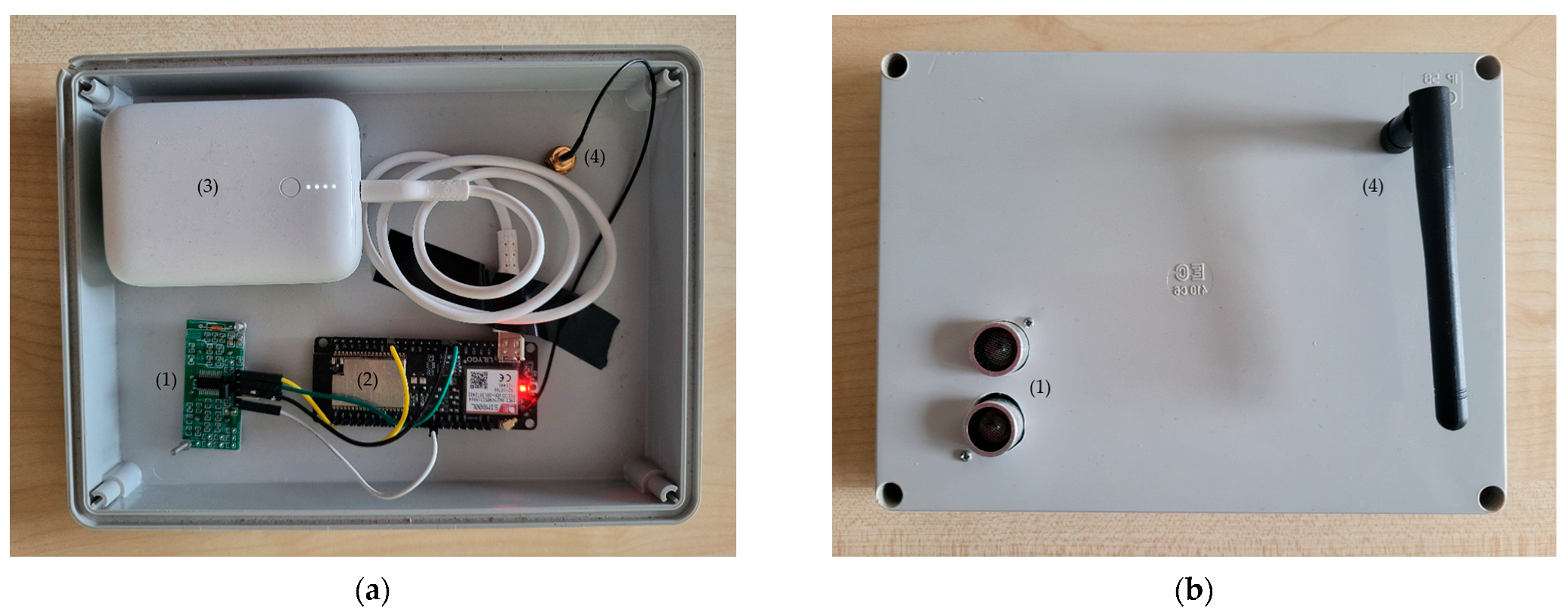
The main parts of the monitoring device (Figure 1) are an ultrasonic distance sensor (1), a microcontroller with an integrated GSM module and SIM card (2), a battery (3), and a GSM antenna (4). The monitoring device is put in an enclosure with appropriate IP protection, as it is placed outdoors and exposed to moisture, dust, wind, and other environmental conditions.

The ultrasonic distance sensor (US-100) serves as a transceiver that generates a pulse, which reflects off an obstacle (e.g., the water surface) and returns to the sensor. The distance is calculated based on the travel time of the pulse and the speed of sound. The speed of sound is affected by the temperature, so it is advisable to choose a sensor with temperature compensation. The microcontroller with the GSM module and SIM card (LILYGO SIM800L; LILYGO, Shenzhen, China) is used as a small programmable computer that continuously reads the sensor values in a loop, connects to the Internet, and sends the data to a server. To save energy, the microcontroller then hibernates until the next measurement cycle. Internet connectivity is provided via the integrated GSM module and SIM card. The battery serves as the power source for the microcontroller, while the GSM antenna, located on the exterior of the enclosure, enables the GSM module to transmit the data. For a prolonged duration of the monitoring, a mini solar panel can be added to charge the battery.

Even when equipped with a small solar panel, the total cost of a single monitoring device can remain below USD 100.

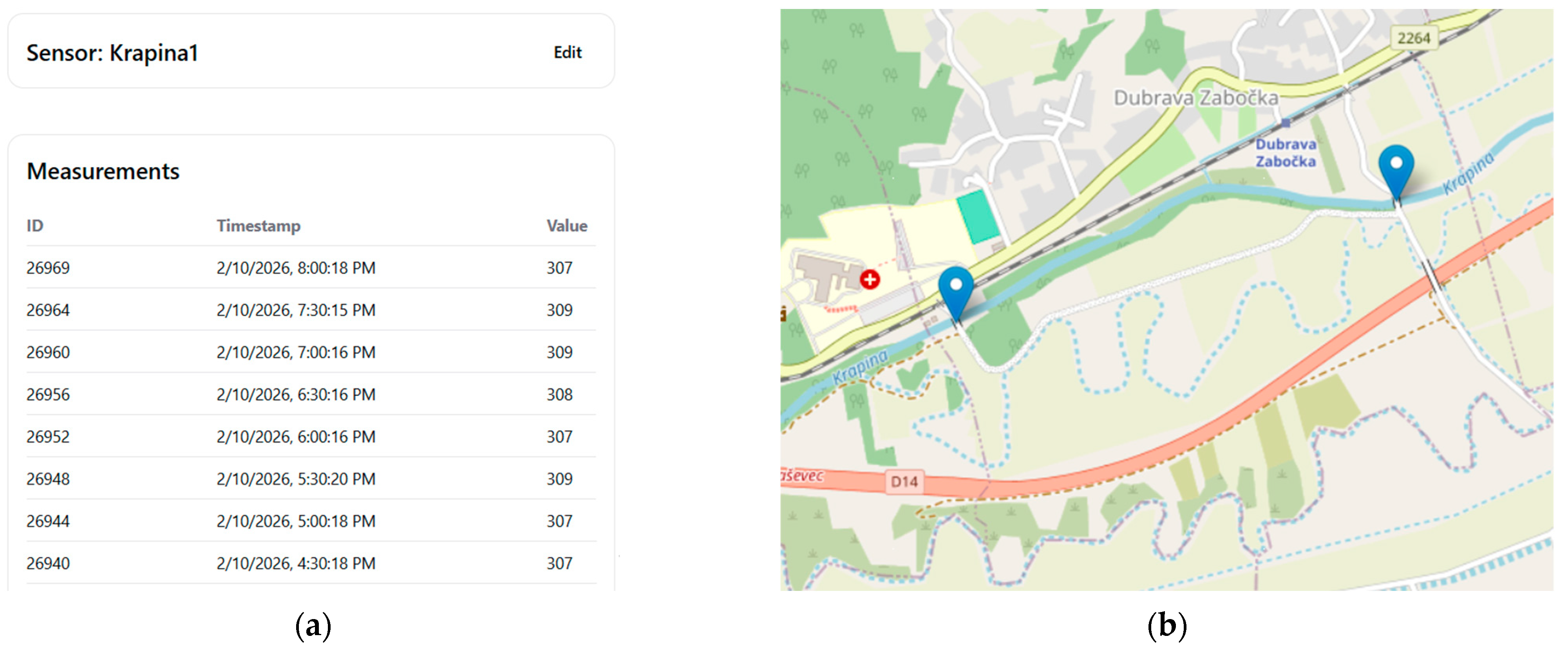
The monitoring devices measure the distance to the water level and transmit the collected data to a server via the Internet. Upon receipt, the server stores the data in a database. A web-based application enables data visualization from the devices and the management of device-related information. For the purpose of development and evaluation of BWLM, a web application was established, comprising a server-side component (API), a database, and a user interface accessible via https://riversensor.com (accessed on 12 February 2026), shown in Figure 2. The web API system was configured using the .NET 6 framework with the C# programming language. The system employs a PostgreSQL database, while the user interface was implemented as a web application using React framework, version 19.

Within the settings of each device, the data acquisition and transmission frequency can be configured and is usually defined in minutes. Time intervals from 15 to 60 min are typically used in river monitoring.

Through the user interface, sensor-specific data presented in tabular form can be accessed. Each transmitted record includes information identifying the sensor from which the measurement originates, along with the recorded value representing the distance between the sensor and the water surface. Each transmitted record is assigned a timestamp to indicate the exact time at which the measurement was acquired.

Based on the geodetically surveyed position of the device, the water levels can be recalculated in absolute values. Time of the measurement and water levels in absolute elevations form the boundary conditions for the hydraulic model.

2.3. Monitoring Location Setup

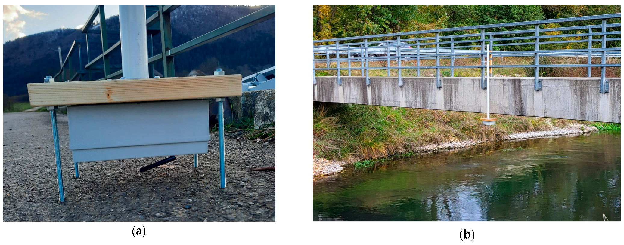
The boundary water level method requires two locations for water level monitoring. The simplest approach to implement BWLM is to identify two bridges in close proximity to each other and to use the bridge railing to mount the sensors above the water surface. For long-term or permanent monitoring, the mounting bracket may be bolted directly to the bridge structure. If no alternative, the measuring devices can be installed on dedicated freestanding supports constructed adjacent to the channel. In any case, the sensors should be placed above the deepest part of the cross-section so they can monitor even the lowest flows (Figure 3).

The components required for simple mounting of the monitoring device on a bridge railing cost up to USD 100.

The optimal reach length is not strictly defined. However, it must be sufficient to allow the detection of a measurable water surface slope at the reach boundaries, which is required for the application of the method. Most manufacturers specify an accuracy of ultrasonic distance sensors of approximately ±1 cm, and additional inaccuracy arises from surface flow turbulence. Considering these factors, a minimum water level difference of approximately 10–15 cm between the upstream and downstream boundaries is required to ensure reliable measurements.

Conversely, if the reach is excessively long, cumulative influences that may alter the discharge along the reach become significant. These include lateral inflows, losses through infiltration, or contributions from the local catchment. To balance these opposing constraints, the target reach length in this study was aimed to range between 0.5 and 2 km.

To establish the hydraulic model, in addition to the boundary cross-sections, several intermediate cross-sections must be geodetically surveyed. The optimal number of surveyed profiles is determined through expert judgment and depends on the characteristics of the reach. In general, a larger number of cross-sections is required for longer and more complex reaches, particularly those with variable bed slope, changing channel width, erosion zones, riffle-pool sequences, or similar morphological irregularities. In this study, between four and seven cross-sections were surveyed per reach, corresponding to a spacing of approximately 100 to 300 m.

3. Results

Two sites were selected for the validation of the Boundary Water Level Method (BWLM). Both sites satisfy the previously defined minimum requirements for method implementation, including adequate reach length to ensure a measurable water surface slope, suitable channel geometry for one-dimensional hydraulic modeling, and the absence of significant lateral inflows or flow losses within the study reach. An additional requirement was the proximity of an official gauging station operated by the State Hydrometeorological Service in Croatia (DHMZ), allowing comparison of the calculated discharges with reference measurements. These conditions allow for a reliable application and evaluation of the proposed method.

3.1. Test Site 1: River Bednja

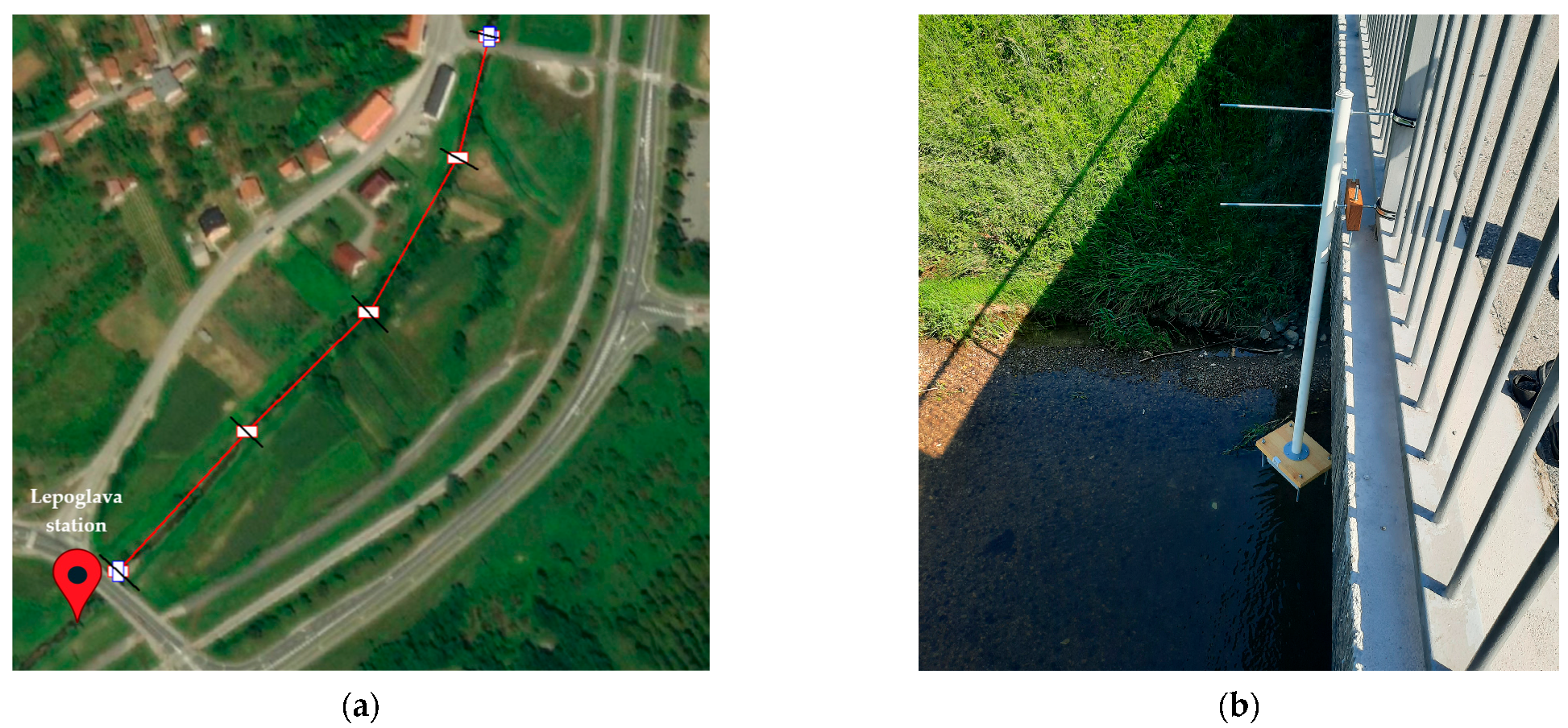
Test site 1 for the Boundary Water Level Method was located on the River Bednja, just downstream of gauging station Lepoglava (Figure 4).

Two bridges located 360 m apart serve as convenient mounting points for the monitoring equipment. In addition to the two boundary cross-sections, three additional cross-sections were geodetically surveyed at an average spacing of 90 m.

Fixed points on both bridge railings were also geodetically surveyed. These points represent the reference elevations from which the sensor positions were determined. The sensors measure the distance from the transducer to the water surface. The water surface elevation in absolute terms is then calculated as the fixed-point elevation minus the vertical offset between the fixed point and the sensor, minus the measured distance to the water surface. Water surface elevations in absolute terms form the stage hydrographs, which represent the boundary conditions for the hydraulic model.

Boundary water levels were continuously measured over a four-day period to capture a small runoff event caused by rainfall in the catchment. The monitoring interval was set to 30 min, and the measured data were transmitted via the Internet to the designated web page. There, the data were stored as time-value pairs in the database. As noted previously, the measured values represent the distance from the sensor to the water surface.

The measured data were exported as a .csv file, after which the recorded values were converted into water surface elevations in absolute terms. Following this conversion, and with a timestamp assigned to each absolute water level value, the boundary condition files were generated.

The boundary conditions and five surveyed cross-sections formed the basis of the one-dimensional (1D) hydraulic model. The hydraulic model was set up using MIKE Hydro River modeling software (DHI, Realease 2017).

The test site on the River Bednja was classified as a clean, winding channel with some pools and shoals, as well as some weeds and stones. This classification suggests Manning’s roughness coefficient (n) in a range from 0.035 to 0.050, with 0.045 being the normal n value [17].

Based on previous modeling experience, a Manning’s roughness coefficient of n = 0.040 was selected as the most representative value for test site 1. A uniform transversal roughness distribution was applied across the river cross-sections to simplify the model setup and allow a clearer evaluation of the influence of Manning’s roughness coefficient. Introducing multiple roughness zones would increase the number of parameters and make it difficult to isolate the effect of individual values on model results. Therefore, a single representative roughness coefficient was used, corresponding to the mean value reflecting both channel and bank characteristics.

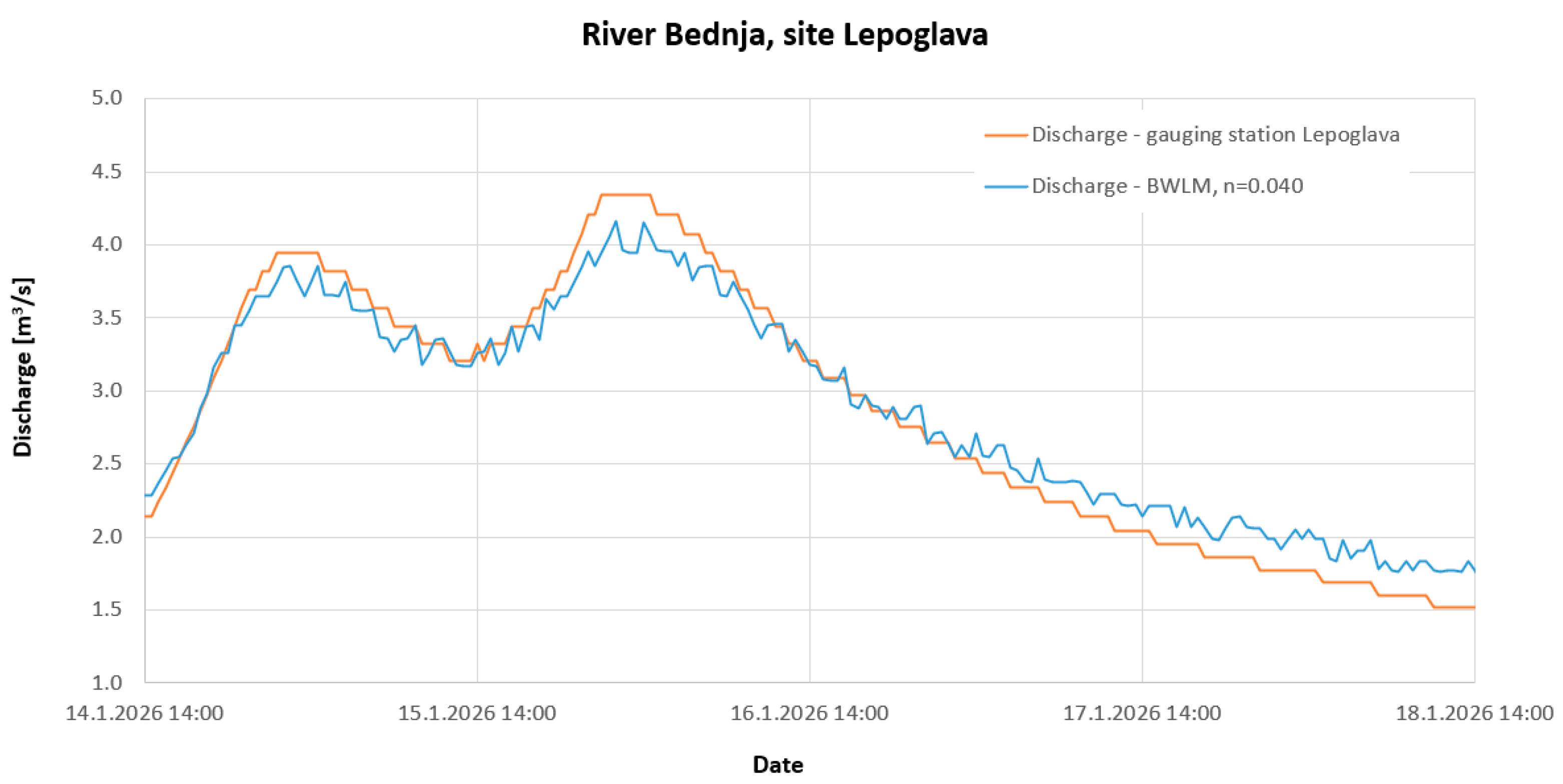
The discharges obtained using the BWLM were compared with those recorded at the Lepoglava gauging station (Figure 5), where water levels are continuously measured and converted to discharge using established rating curves. For the present monitoring period, discharges were calculated using the 2024 rating curve, the most recent one available.

The results indicate that the flood wave obtained using the BWLM and that recorded at the gauging station are qualitatively consistent. When using n = 0.040, the peak discharge is slightly underestimated by the BWLM. The gauging station recorded a peak discharge of 4.30 m³/s, whereas the BWLM simulation yielded 4.16 m³/s, representing an absolute error of 0.14 m³/s, or 4.1%.

In contrast, low discharges are slightly overestimated by the BWLM. The gauging station recorded a minimum discharge of 1.44 m³/s, while the BWLM simulation yielded 1.69 m³/s, corresponding to an absolute error of 0.25 m³/s, or 17.7%. This larger relative error at low discharges can be attributed to several factors. First, small absolute differences in discharge result in larger percentage errors when reference values are low. In addition, hydraulic conditions at low flows are more sensitive to uncertainties in water level measurements and channel roughness, which can significantly influence discharge estimates. Furthermore, minor variations in channel geometry and flow resistance, which are less pronounced at higher flows, may have a greater relative impact under low-flow conditions.

Overall, during the four-day monitoring period and assuming n = 0.040, the mean absolute percentage error (MAPE) between the BWLM-estimated discharges and those recorded at the gauging station was 6.7%.

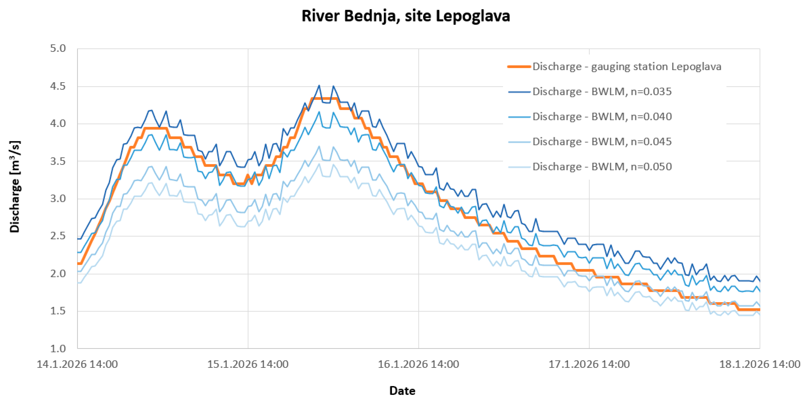
Three additional hydraulic simulations were conducted using different n values within the proposed range of 0.035–0.050 (Figure 6), and the sensitivity analysis was performed to evaluate the influence of hydraulic roughness on discharge calculation. While channel geometry and boundary water levels were determined from field measurements, Manning’s roughness coefficient has to be estimated. The hydraulic model was run, varying only the roughness coefficient while keeping all other parameters constant. The resulting discharges were compared in terms of mean, peak, and low-flow values to assess the sensitivity of the method to uncertainty in hydraulic roughness.

Sensitivity analysis (SA) was conducted using multiple performance indicators to evaluate the sensitivity of BWLM discharge estimates to variations in Manning’s roughness coefficient (n). The root mean square error (RMSE) and Nash–Sutcliffe efficiency (NSE) were used to assess the agreement between simulated and observed discharge time series in terms of overall model performance and absolute deviations. The mean absolute percentage error (MAPE) was used to quantify the average relative deviation between simulated and observed discharges, while percent bias (PBIAS) was used to evaluate the tendency of the model to systematically overestimate or underestimate discharge. Finally, percentage errors for minimum and maximum discharge (Q_max and Q_min) were used to assess the influence of roughness on low-flow and peak-flow conditions of the modeled event (

Table 1. Sensitivity analysis indicators for BWLM discharge estimates under different Manning’s roughness coefficients for test site 1.

Manning’s n	RMSE (m3/s)	NSE (-)	MAPE (%)	PBIAS (%)	Qmax Error (%)	Qmin Error (%)
0.035	0.29	0.90	12.1	8.6	4.0	26.9
0.040	0.18	0.96	6.7	1.2	−4.1	17.7
0.045	0.38	0.83	9.0	−11.0	−14.7	4.7
0.050	0.53	0.66	14.3	−19.3	−20.0	−3.7

).

The sensitivity analysis indicates a clear dependence of the calculated discharges on Manning’s roughness coefficient. The best agreement with the measured discharges was obtained for n = 0.040, which yielded the lowest RMSE (0.18 m³/s) and the highest NSE (0.96), indicating very good overall model performance. This is further supported by the lowest mean absolute percentage error (MAPE = 6.7%) and a near-zero percent bias (PBIAS = 1.2%).

Lower roughness (n = 0.035) resulted in systematic overestimation of discharge (PBIAS = 8.6%), while higher roughness values (n ≥ 0.045) led to increasing underestimation, with PBIAS reaching −19.3% for n = 0.050. This trend is also reflected in the NSE and RMSE values, which show a progressive deterioration in model performance as the roughness coefficient deviates from the optimal value.

Peak discharge errors follow a similar pattern, shifting from slight overestimation at lower roughness values to increasing underestimation as roughness increases. In contrast, the largest deviations were observed for low flows, where errors ranged from 26.9% to −3.7%. This indicates that the model results are more sensitive to Manning’s roughness coefficient under low-flow conditions than during peak discharge.

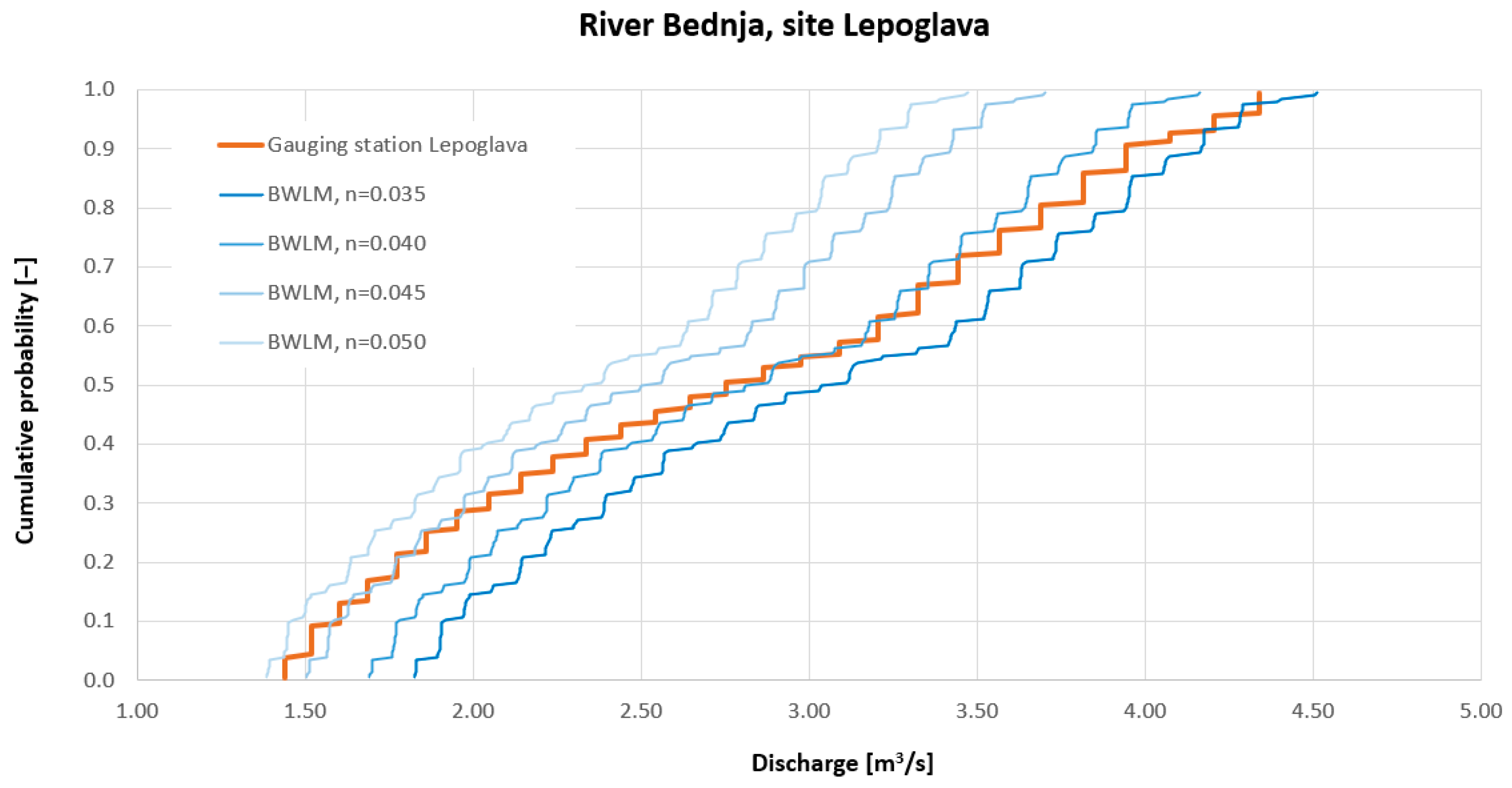
To further examine the distributional agreement between simulated and observed discharges, cumulative distribution functions (CDFs) were also analyzed (Figure 7).

The empirical cumulative distribution functions (CDFs) of observed and simulated discharge indicate a clear sensitivity of model performance to the Manning’s roughness coefficient. Among the tested scenarios, n = 0.040 shows the best overall agreement with the observed distribution, closely reproducing the cumulative behaviour across the monitored range of discharges. In contrast, n = 0.035 results in a systematic overestimation of discharge values, shifting the CDF toward higher flows, while n = 0.045 and n = 0.050 progressively underestimate discharge and compress the upper tail of the distribution. The observed differences are most pronounced in the low- and high-flow regions, highlighting the importance of appropriate roughness calibration for accurate reproduction of both frequent low-flow conditions and less frequent higher-flow events. Overall, the CDF analysis confirms n = 0.040 as the optimal parameter for the studied reach.

3.2. Test Site 2: River Krapina

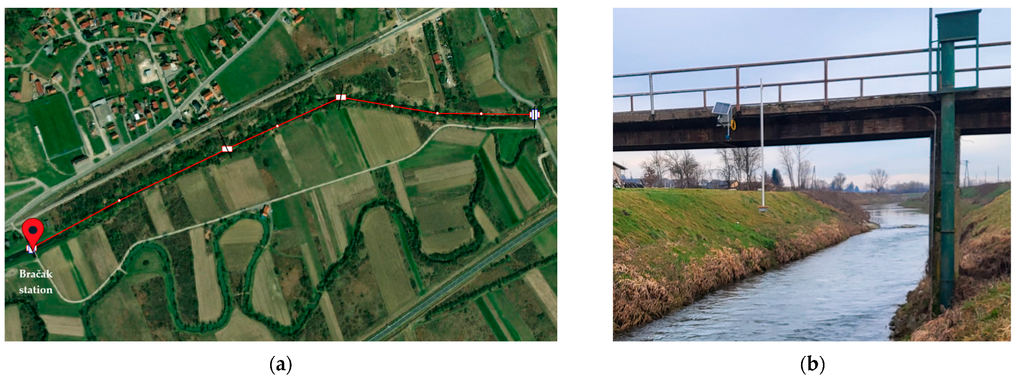
Test site 2 for the Boundary Water Level Method was located on the River Krapina upstream of the gauging station Bračak (Figure 8).

Again, two bridges situated 1080 m apart were used as convenient mounting points for the monitoring equipment. In addition to the boundary cross-sections at the bridges, two more cross-sections were geodetically surveyed at an average spacing of 360 m.

This time, over a period of seven days, boundary water levels were continuously recorded to capture a minor runoff event triggered by rainfall in the catchment. Readings were taken every 30 min.

The River Krapina test site was characterized as a clean, straight channel with some pools and shoals. Based on this channel type, Manning’s roughness coefficient n is estimated to range from 0.030 to 0.040, with a representative value of 0.035 [17].

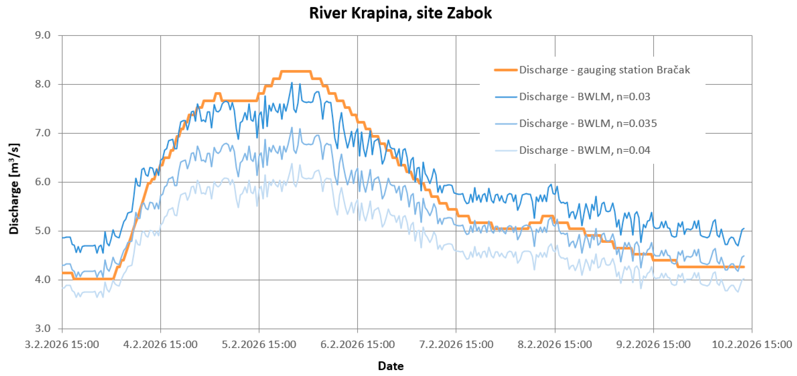
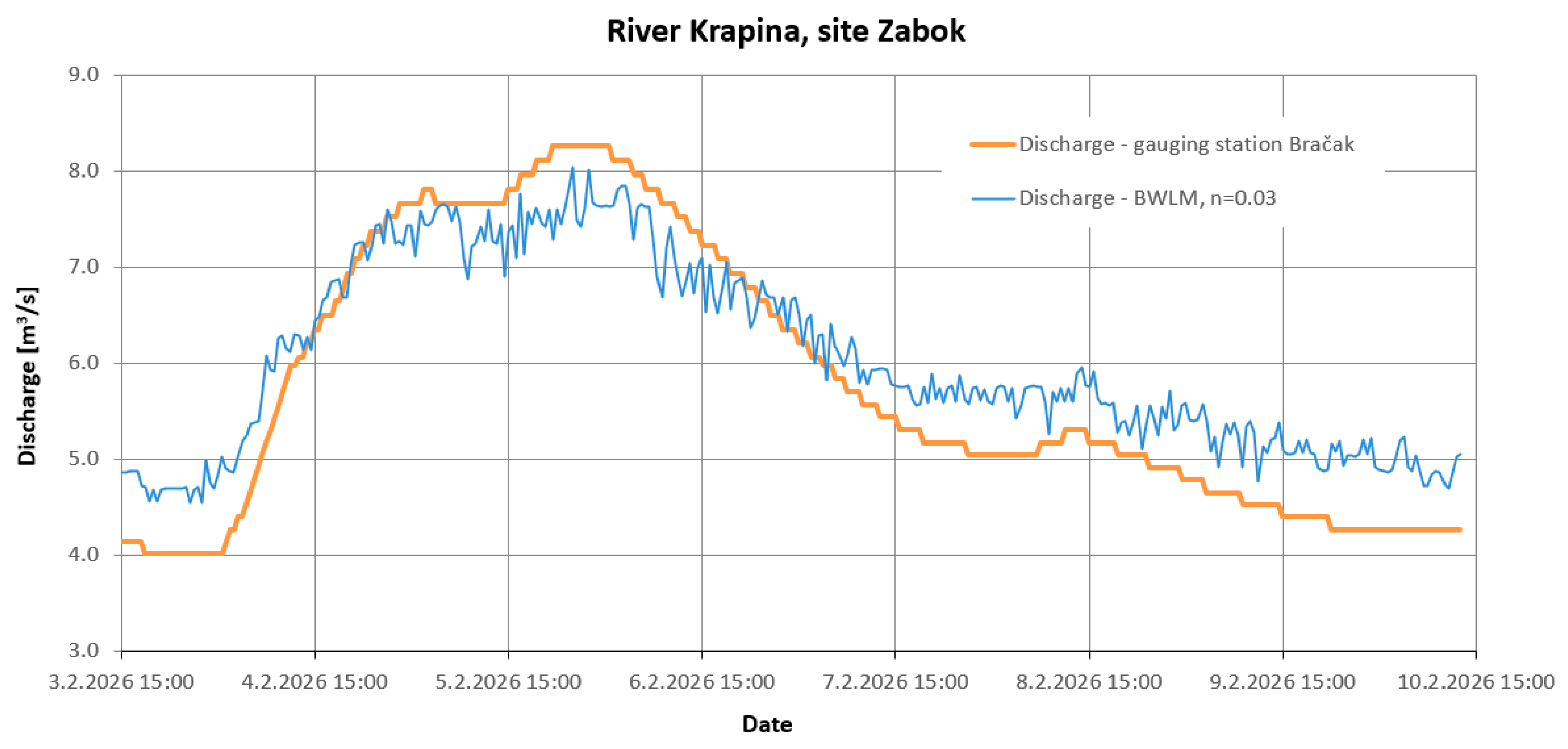
Drawing on prior modeling experience, Manning’s roughness coefficient of n = 0.030 was chosen as the most representative value for test site 2, again implementing a uniform transversal roughness distribution across the river cross-section. Discharges estimated by the BWLM were compared with measurements from the Bračak gauging station (Figure 9), where water levels are continuously monitored and converted to discharge using the most recent available rating curve, which dates from 2024.

The results for the test site 2 also show that the flood wave simulated by the BWLM is qualitatively consistent with that observed at the gauging station. Using n = 0.030, the BWLM underestimates the peak discharge, while overestimating low discharges. The gauging station Bračak measured a peak of 8.26 m³/s, the BWLM simulation produced 8.04 m³/s, resulting in an absolute error of 0.22 m³/s, or 2.6%.

The lowest discharge measured by the gauging station was 4.02 m³/s, and the corresponding discharge by the BWLM was 4.55 m³/s, which translates into an absolute error of 0.53 m³/s, or 13.2%.

Similar to the first test site results, the relative error is more pronounced under low-flow conditions. Again, this can be partly explained by the fact that smaller reference discharge values lead to larger percentage errors for comparable absolute deviations. In addition, the method is more sensitive at low flows, where uncertainties in water level measurements and roughness estimation have a greater influence on the calculated discharge. In contrast, higher flows are less affected by such uncertainties, resulting in better agreement between simulated and observed peak values.

Overall, during the seven-day monitoring period and assuming n = 0.030, the mean absolute percentage error (MAPE) between the BWLM-estimated discharges and those recorded at the gauging station was 9.3%.

Two additional hydraulic simulations were carried out using different n values within the proposed range of 0.030–0.040 in order to perform a sensitivity analysis and evaluate the effect of hydraulic roughness on discharge estimation (Figure 10). The model was therefore executed by varying only the roughness coefficient, while all other parameters were kept constant. The resulting discharges were evaluated in terms of mean, peak, and low-flow values to quantify the sensitivity of the method to uncertainty in hydraulic roughness.

Sensitivity analysis (SA) was conducted using the same six performance indicators (RMSE, NSE, MAPE, PBIAS, Q_max error and Q_min error) to evaluate the sensitivity of BWLM discharge estimates to variations in Manning’s roughness coefficient (

Table 2. Sensitivity analysis indicators for BWLM discharge estimates under different Manning’s roughness coefficients for test site 2.

Manning’s n	RMSE (m3/s)	NSE (-)	MAPE (%)	PBIAS (%)	Qmax Error (%)	Qmin Error (%)
0.030	0.54	0.85	9.3	0.4	−2.6	13.2
0.035	0.72	0.74	7.7	−10.9	−13.7	0.7
0.040	1.19	0.28	15.4	−20.1	−22.7	−9.5

).

The sensitivity analysis for test site 2 also indicates a clear influence of Manning’s roughness coefficient on the calculated discharges. The best overall agreement with the measured discharges was obtained for n = 0.030, which yielded the lowest RMSE (0.54 m³/s) and the highest NSE (0.85), indicating good agreement between simulated and observed discharge time series. This configuration also resulted in a near-zero bias (PBIAS = 0.4%) and a relatively small peak discharge error (−2.6%), although the low-flow error remained moderate (13.2%).

A slightly lower MAPE was obtained for n = 0.035 (7.7%); however, this configuration showed reduced overall performance, with a lower NSE (0.74) and higher RMSE (0.72 m³/s), accompanied by a noticeable negative bias (PBIAS = −10.9%) and increased underestimation of peak discharge (−13.7%).

Further increasing the roughness coefficient to n = 0.040 led to a substantial deterioration in model performance, as reflected by a marked decrease in NSE (0.28) and a significant increase in RMSE (1.19 m³/s). This is consistent with the higher MAPE (15.4%) and strong negative bias (PBIAS = −20.1%), as well as pronounced underestimation of both peak discharge (−22.7%) and low flows (−9.5%).

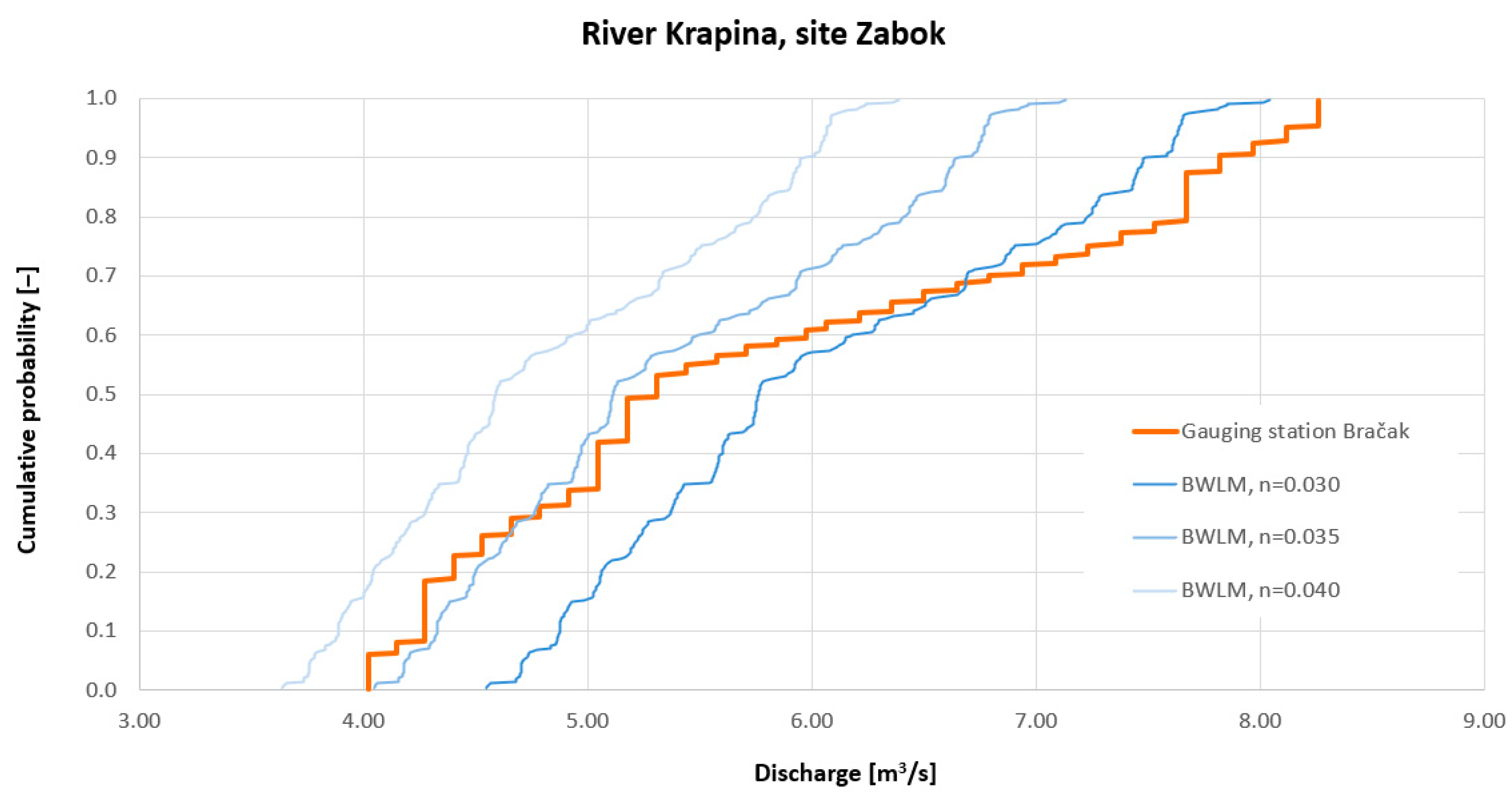
In addition, cumulative distribution functions (CDFs) were evaluated to assess the agreement between simulated and observed discharge distributions (Figure 11).

The empirical cumulative distribution functions (CDFs) for test site 2 further confirm the sensitivity of the model to the selected Manning’s roughness coefficient. The results indicate that n = 0.030 provides the best overall agreement with the observed discharge distribution, particularly across the high to medium flow ranges. Although this configuration does not provide the closest match to the lowest discharge values, it more effectively captures the overall variability and extent of the observed distribution. In contrast, n = 0.035 and n = 0.040 progressively shift the simulated distributions toward lower discharge values, resulting in an underestimation of flow and a compression of the upper tail. Overall, the CDF analysis supports the selection of n = 0.030 as the most appropriate roughness coefficient for test site 2.

4. Discussion

The application of the one-dimensional (1D) hydraulic model in this study was based on the assumption of gradually varied flow conditions and predominantly one-dimensional flow behavior within the selected river reaches. The key modelling parameters include channel geometry, boundary water levels, and Manning’s roughness coefficient, of which the latter introduces the highest degree of uncertainty. While channel geometry and boundary conditions were derived directly from field measurements, the roughness coefficient had to be estimated based on literature, field observations and prior experience.

The sensitivity analyses at both test sites demonstrate that the calculated discharges are strongly influenced by the selected Manning’s roughness coefficient. In both cases, increasing the roughness coefficient resulted in progressively lower simulated discharges, which is consistent with the physical relationship between flow resistance and conveyance. The results also indicate that relatively small variations in Manning’s n can produce noticeable differences in discharge estimates. Even when roughness values were selected from the same channel condition category, the use of minimum and maximum recommended values resulted in substantially different discharge estimates. This finding highlights the inherent uncertainty associated with roughness estimation and emphasizes the importance of careful parameter selection in hydraulic modeling.

Although the BWLM provided reasonably good agreement with observed discharges at both sites, the sensitivity analysis shows that inaccurate roughness assumptions may lead to systematic overestimation or underestimation of discharge. Therefore, due care should be taken when applying the method in ungauged or poorly studied basins, where direct calibration against measured discharges is not available.

Compared with some other conventional discharge measurement techniques, the boundary water level method (BWLM) offers several practical advantages. One of its main strengths is the relatively low cost of implementation, as the monitoring device and mounting components can be assembled for less than USD 200 per device. In addition, the system enables continuous and contactless water level measurements and provides real-time data transmission via the Internet. Once installed, the method allows discharge to be estimated immediately through the hydraulic model without the need for repeated field measurements. The integration of a hydraulic model also enables additional analyses, such as the evaluation of hydraulic conditions along the modeled reach.

However, several limitations should also be considered. The method requires two monitoring locations to define the boundary conditions, which may restrict its application in river reaches where suitable mounting structures, such as bridges, are not available at appropriate distances. Alternatively, standalone mounting structures can be installed for the monitoring device, although this may increase both installation costs and technical complexity. Furthermore, the accuracy of water level measurements depends on the performance of the ultrasonic sensor used in the monitoring device. Ultrasonic sensors are generally more susceptible to measurement noise and environmental influences compared with radar or pressure-based sensors, which may introduce additional uncertainty into the calculated discharges. In addition, the applicability of the method depends on the hydraulic characteristics of the selected reach. River sections with very mild slopes may not provide sufficient water level differences for reliable boundary definition, while longer reaches may be affected by cumulative influences such as lateral inflows or losses, leading to inconsistencies in discharge along the reach. Similarly, conditions involving backwater effects or rapidly varying flow may violate the underlying modeling assumptions and reduce the reliability of the results. Despite these limitations, the BWLM approach represents a promising low-cost alternative for discharge estimation, particularly in small rivers and poorly gauged basins.

Future research will extend the present analysis to multiple sites, flood events, and longer time periods to further assess the robustness and transferability of the proposed approach under a broader spectrum of hydraulic conditions and flow regimes.

References

1. World Meteorological Organization. Guide to Hydrological Practices, Volume I, 6th ed.; WMO-No. 168; World Meteorological Organization: Geneva, Switzerland, 2008. [Google Scholar]
2. Segovia-Cardozo, D.A.; Rodríguez-Sinobas, L.; Canales-Ide, F.; Zubelzu, S. Design and field implementation of a low-cost, open-hardware platform for hydrological monitoring. Water 2021, 13, 3099. [Google Scholar] [CrossRef] [Scilit]
3. Garbossa, L.H.P.; Novaes, A.L.; Lapa, K.R. Low-Cost Automation for Hydrological Monitoring in Water Resources Management. Proceedings 2020, 48, 29. [Google Scholar]
4. Dobriyal, P.; Badola, R.; Tuboi, C.; Hussain, S.A. A review of methods for monitoring streamflow for sustainable water resource management. Appl. Water Sci. 2017, 7, 2617–2628. [Google Scholar] [CrossRef] [Scilit]
5. World Meteorological Organization. Manual on Stream Gauging; Volume I: Fieldwork. WMO-No. 1044; World Meteorological Organization: Geneva, Switzerland, 2010. [Google Scholar]
6. ISO 1070:2018; Hydrometry—Slope-Area Method. International Organization for Standardization (ISO): Geneva, Switzerland, 2018.
7. Stewart, A.M.; Callegary, J.B.; Smith, C.F.; Gupta, H.V. Use of the continuous slope–area method to estimate runoff in a network of ephemeral channels, southeast Arizona, USA. J. Hydrol. 2012, 472–473, 148–158. [Google Scholar] [CrossRef] [Scilit]
8. Lüthi, B.; Philippe, T.; Peña-Haro, S. Mobile device app for small open-channel flow measurement. In Proceedings of the 7th International Congress on Environmental Modelling and Software, San Diego, CA, USA, 15–19 June 2014; Ames, D.P., Quinn, N.W.T., Rizzoli, A.E., Eds.; International Environmental Modelling and Software Society: San Diego, CA, USA, 2014. [Google Scholar]
9. Bjerklie, D.M.; Birkett, C.M.; Jones, J.W.; Carabajal, C.; Rover, J.A.; Fulton, J.W.; Garambois, P.-A. Satellite remote sensing estimation of river discharge: Application to the Yukon River, Alaska. J. Hydrol. 2018, 561, 1000–1018. [Google Scholar] [CrossRef] [Scilit]
10. Pizarro, A.; Valera-Gran, D.; Navarrete-Muñoz, E.-M.; Dal Sasso, S.F. The Use of Unmanned Aerial Systems for River Monitoring: A Bibliometric Analysis Covering the Last 25 Years. Hydrology 2024, 11, 80. [Google Scholar] [CrossRef] [Scilit]
11. Strelnikova, D.; Perks, M.T.; Dal Sasso, S.F.; Pizarro, A. River flow monitoring with unmanned aerial systems. In Unmanned Aerial Systems for Monitoring Soil, Vegetation, and Riverine Environments; Earth Observation: Greenbelt, MA, USA, 2023; pp. 231–269. [Google Scholar]
12. Alimenti, F.; Bonafoni, S.; Gallo, E.; Palazzi, V.; Gatti, R.V.; Mezzanotte, P.; Roselli, L.; Zito, D.; Barbetta, S.; Corradini, C.; et al. Noncontact measurement of river surface velocity and discharge estimation with a low-cost Doppler radar sensor. IEEE Trans. Geosci. Remote Sens. 2020, 58, 5195–5207. [Google Scholar] [CrossRef] [Scilit]
13. Costa, J.E.; Cheng, R.T.; Haeni, F.P.; Melcher, N.; Spicer, K.R.; Hayes, E.; Plant, W.; Hayes, K.; Teague, C.; Barrick, D. Use of radars to monitor stream discharge by noncontact methods. Water Resour. Res. 2006, 42, 14. [Google Scholar] [CrossRef] [Scilit]
14. Vyas, J.K.; Perumal, M.; Moramarco, T. Non-contact discharge estimation at a river site by using only the maximum surface flow velocity. J. Hydrol. 2024, 638, 131505. [Google Scholar] [CrossRef] [Scilit]
15. DHI. MIKE 1D: DHI Simulation Engine for 1D River and Urban Modelling; Reference Manual 2025; DHI: Hørsholm, Denmark, 2025. [Google Scholar]
16. U.S. Army Corps of Engineers. HEC-RAS: Hydraulic Reference Manual; Version 6.6; Hydrologic Engineering Center (HEC), U.S. Army Corps of Engineers: Davis, CA, USA, 2024. [Google Scholar]
17. Chow, V.T. Open-Channel Hydraulics; McGraw-Hill: New York, NY, USA, 1959. [Google Scholar]
Figure 1. Monitoring device components: (a) Inside view; (b) Bottom view.
Hydrology 13 00116 g001
Figure 2. Web application for data collection: (a) Data view; (b) Map view.
Hydrology 13 00116 g002
Figure 3. Water level monitoring: (a) Monitoring device; (b) mounting on the bridge railings.
Hydrology 13 00116 g003
Figure 4. Test site 1: (a) River Bednja reach in model setup and position of gauging station Lepoglava; (b) Monitoring device on the upstream bridge location.
Hydrology 13 00116 g004
Figure 5. Comparison of BWLM discharges and the Lepoglava gauging station discharges.
Hydrology 13 00116 g005
Figure 6. BWLM test site 1 discharge hydrographs for varying Manning’s roughness coefficients.
Hydrology 13 00116 g006
Figure 7. Empirical cumulative distribution functions (CDFs) of observed and BWLM simulated discharge for varying Manning’s roughness coefficients for test site 1.
Hydrology 13 00116 g007
Figure 8. Test site 2: (a) River Krapina reach in model setup and position of gauging station Bračak; (b) Monitoring device on the downstream bridge location.
Hydrology 13 00116 g008
Figure 9. Comparison of BWLM discharges and the Bračak gauging station discharges.
Hydrology 13 00116 g009
Figure 10. BWLM test site 2 discharge hydrographs for varying Manning’s roughness coefficients.
Hydrology 13 00116 g010
Figure 11. Empirical cumulative distribution functions (CDFs) of observed and BWLM simulated discharge for varying Manning’s roughness coefficients for test site 2.
Hydrology 13 00116 g011