Article

Spatiotemporal Variation in Land Use/Land Cover and Its Driving Causes in a Semiarid Watershed, Northeastern China

1
School of Environment, Liaoning University, Shenyang 110036, China
2
State Key Laboratory of Water Cycle and Water Security, China Institute of Water Resources and Hydropower Research, Beijing 100038, China
*
Author to whom correspondence should be addressed.
Hydrology 2026, 13(1), 42; https://doi.org/10.3390/hydrology13010042 (registering DOI)
Submission received: 18 November 2025 / Revised: 10 January 2026 / Accepted: 20 January 2026 / Published: 22 January 2026
(This article belongs to the Section Hydrology–Climate Interactions)

Abstract

The West Liaohe River Basin, a core arid region in Northeast China, faces a significant evaporation–precipitation imbalance and exhibits fragmented land systems, epitomized by the Horqin Sandy Land. Integrating three decades of land use/land cover (LULC) data with meteorological, ecological, and socioeconomic variables, we employed obstacle diagnosis and structural equation modeling (SEM) to elucidate the spatiotemporal dynamics and drivers of LULC transformations. The results demonstrate the following: (1) Land use exhibited a spatially heterogeneous pattern, with forests, shrubs, and grasslands predominantly concentrated in the northwest and southwest. (2) Vegetation coverage significantly increased from 53.15% in 1990 to 61.32% in 2020, whereas cropland and sandy land areas declined. While the overall basin landscape underwent a marked increase in fragmentation. (3) Human activities were the dominant contributor of LULC changes, particularly for cropland conversion, with key determinants such as population and GDP showing negative path coefficients of −0.59 and −0.77, respectively. Climate change was a secondary contributor, with precipitation exerting a strong positive path coefficient (0.63) that was particularly pronounced during the conversion of grassland to forest. These findings offer a scientific basis for land management, ecological restoration strategies, and water resource utilization in the basin.

1. Introduction

Socioeconomic development drives dynamic changes in fundamental natural resources such as water and land. Land use/land cover (LULC) serves as a primary indicator and nexus of these transformations [1,2]. Globally, LULC has shifted from forests to croplands and urban areas over the past 300 years [1,3]. The contraction of forest area contributes to climate change and ecological imbalance [4], and its expansion typically reduces water yield and soil erosion while an increase in urban elevates the risk of urban flooding [5]. In China, forest area decreased by 22% (from 176.1 to 137.7 million ha), whereas cropland increased by 42% (from 94.9 to 134.7 million ha) and urban land expanded 1075% (from 1.6 to 18.8 million ha) between 1700 and 2005 [6]. China has undertaken substantial vegetation-restoration efforts in recent decades, including the Three-North Shelterbelt Development Program and the Grain for Green Project [7]. The resulting increase in vegetation cover has delivered considerable ecological benefits; for example, carbon sequestration in the Three-North Shelterbelt increased by an average of 1.92% per year from 1990 to 2015 [8]. In arid basins, the expansion of forests and grasslands is a key indicator of terrestrial ecological restoration [9,10], and can mitigate soil desertification and enhance regional precipitation. By contrast, urban expansion increases environmental burdens and water pollution [11]. Therefore, LULC changes have significant impacts on economic development, water security, and the hydrological cycle at the basin scale [12,13,14], and rational land development can enable the coordination of high-quality development and high-level protection [15]. Analyzing long-term LULC dynamics at regional or basin scales provides critical insights to guide future ecological integrity, socioeconomic development, resource endowments, and industrial planning [2,16].
In recent years, fundamental research on LULC at basin scale has predominantly focused on analyzing spatiotemporal process, landscape pattern dynamics, and its conversion across different periods [17,18]. Exploring the driving factors of LULC changes is an effective approach to addressing the water problem in watershed scale [14]. Yao et al. [19] calculated the transfer matrix of LULC in Yanhe River Basin, revealing that population growth and urbanization rate were the primary drivers of land use change. Zhang et al. [20] revealed that the driving factors of land use change could include a conceptual form; social economy and the Gross Domestic Product (GDP) had a negative explanatory variable for cropland in Xixian New Area. Using transfer matrices and statistical methods, Lin et al. [21] examined the relationships between precipitation and LULC variations in forest areas. However, earlier methodological approaches for investigating the drivers of LULC change predominantly relied on relational analysis [19], traditional questionnaire surveys [22], key informant interviews (KII) [23], focus group discussions (FGD) [24], geographical detectors [25], and ordinary least squares and spatial econometric model [26]. These methods are often limited by challenges such as difficulties in obtaining historical data, inconsistencies in survey responses, and the complex interdependencies among influencing factors [11]. In particular, they struggle to accurately identify and quantify latent variables (e.g., climate drivers) that often require integration of multiple dominant variables for effective representation. Therefore, the migration of structural equation modeling (SEM), a method traditionally used in sociological analysis, to the investigation of land use change drivers can more effectively elucidate the relationships between latent and directly observed variables [27]. SEM provides a global perspective on broader structural relationships [28].
The West Liaohe River Basin (WLRB) is a critical part of northern China’s ecological barrier [29,30,31], characterized by high ecological sensitivity and fragility [32,33]. It is an agro-pastoral transition zone, with primary agricultural and livestock production [34,35]. Therefore, analyzing the spatiotemporal dynamics of LULC in the WLRB not only reveals the impacts of human activities and climate change but also provides valuable insights for ecological planning and land management. Such research holds significant and far-reaching implications for future evolution and development. To advance rational water allocation, guide ecological conservation in the Horqin Sandy Land, and promote sustainable agriculture and river ecosystem revitalization in the WLRB, we conducted a comprehensive study. Based on a multidimensional dataset (1990–2020) of land use, hydro-meteorology, and socioeconomic drivers—encompassing precipitation, soil erosion amount (SEA), urbanization rate (UR), and water consumption per unit of industry (UIW)—our analysis (1) quantified spatiotemporal land use dynamics and landscape pattern fragmentation; (2) identified key driving factors via a diagnostic model; and (3) elucidated the interactions among these drivers through SEM.

2. Materials and Methods

2.1. Study Area

The West Liaohe River is the largest tributary of the Liaohe River [36], located in northeastern China, and its southern and northern source is Laoha River and Xilamulun River, respectively. The main channel of the West Liaohe River spans approximately 449 km and flows through Chengde (Hebei province), Chifeng, and Tongliao (Inner Mongolia), mainly including Horqin District, Kailu and Changtu country, and Shuangliao City [35,37].
The area of WLRB is about 136,000 km2 (116°36′ E~124°35′ E, 40°05′ N~45°13′ N), accounting for 43% of the total Liaohe River Basin [34,38]. Its terrain decreases from 2055 masl to 84 masl from west to east (Figure 1). The average annual precipitation in the basin is 420.1 mm, while the evaporation is 1564.2 mm. The WLRB lies at the transitional zone between the southeastern edge of the Mongolian Plateau and the Northeast China Plain [32].

2.2. Data Sources

The data used in this paper mainly include historical land use data [39], historical meteorological data, water resources data, socioeconomic data, and statistical data of the WLRB (Table 1).

2.3. Methods

This study first analyzed the changes in the land transition matrix for the WLRB from 1990 to 2020. The changing trends in the regional landscape pattern were assessed using landscape indices [39]. Additionally, the main driving factors affecting land cover in the basin were identified using the obstacle diagnosis model [40,41]. Finally, the relationships between LULC, climate change, human activities, and ecological environment were quantified through SEM [42].

2.3.1. Land Use Transition Matrix

The land use transition matrix reveals the evolution trends of land use types. By establishing the matrix relationship between the initial and the final type of various land use types in the region, the evolution direction and change area of various land use types would be shown [42,43].
L a b = L 11 L 1 n L n 1 L n n
where Lab is the change area of land use type, n denotes the number of transferred land use types, and a and b represent the land use types at the beginning and end of the study period, respectively.

2.3.2. Landscape Pattern Index

To characterize the spatiotemporal outcomes of LULC changes in WLRB, we analyzed the landscape pattern index that captures the degree of fragmentation, shape complexity, dispersion, and aggregation of patches. Based on previous studies [43,44], different indices (Appendix A, Table A1) were selected to analyze the dominant landscape types and the interannual changes, correlation between the dominant landscape types and landscape diversity over different periods in the study area. These calculations were performed using Fragstats4.2 [45,46].
In Fragstats4.2, six types of landscape indices were calculated, including patch type level and landscape level. Based on the landscape pattern characteristics and practical considerations of the study area, the ecological landscape pattern index was mainly analyzed at both the patch type and landscape levels, with seven indices selected from the patch type level and eight indices from the landscape level.

2.3.3. Obstacle Factor Diagnosis

The obstacle degree is a diagnostic metric derived from a multi-criteria framework. It is a diagnostic approach used to identify which factors act as the largest ‘obstacles’ (or limiting factors) to a target outcome. An obstacle degree value is calculated for each factor (Equation (2)), where a higher value indicates that the factor is more hindering.
O i j = W j 1 y i j j = 1 m W j 1 y i j
where Oij represents the j th index obstacle degree of the i th object, Wj is the weight of obstacle factor, and (1 − yij) is the gap between the index and the index target.
To better understand the effects of target factors on the LULC of the WLRB, this study analyzed a set of 20 indicators spanning meteorological, socioeconomic, as well as natural and ecological dimensions (Appendix A, Table A2). These 20 indicators include precipitation [47], evaporation [48], population [49], GDP [50], SEA [41], net ecosystem productivity (NEP) [51], UR [49], soil and water conservation ratio (SWC) [52], and UIW [50]. This study employed obstacle factor diagnosis to assess the degree of obstruction for 20 target factors influencing LULC and its main internal control factors.

2.3.4. Structural Equation Modeling

The SEM is a statistical method that combines factor analysis, regression analysis, and path analysis. It is a method used to establish, estimate, and test models of causal relationship. Compared to the traditional analysis method, the SEM can explain the latent variations in the model, such as a relatively abstract concept, which could be combined with observed variables (measured directly). Based on the obstacle factor diagnosis analysis, key indicators with significant influence were selected from the 20 observed variables to form three latent variables: climate factors, ecological–environmental factors, and human activity factors. The WLRB was delineated into several sub-basins and catchments, giving a total sample size of 228. For these catchments, parameters were estimated by the method of maximum likelihood. To ensure high factor loadings for each latent variable, Cronbach’s alpha was applied to assess the internal consistency of each group (greater than 0.7 is generally considered to indicate acceptable reliability). The analysis in this study was conducted using Amos software [31,42]. To assess model fit, comparative fit index (CFI) and root mean square error of approximation (RMSEA) were used to test the model [53]. Combined with the model’s sample size and number of indicators, model fit was regarded as acceptable with CFI > 0.85 and RMSEA < 0.09, while a path hypothesis was supported by a significance level of p < 0.05.

3. Results

3.1. Spatiotemporal Variation Characteristics of Land Use/Land Cover in WLRB

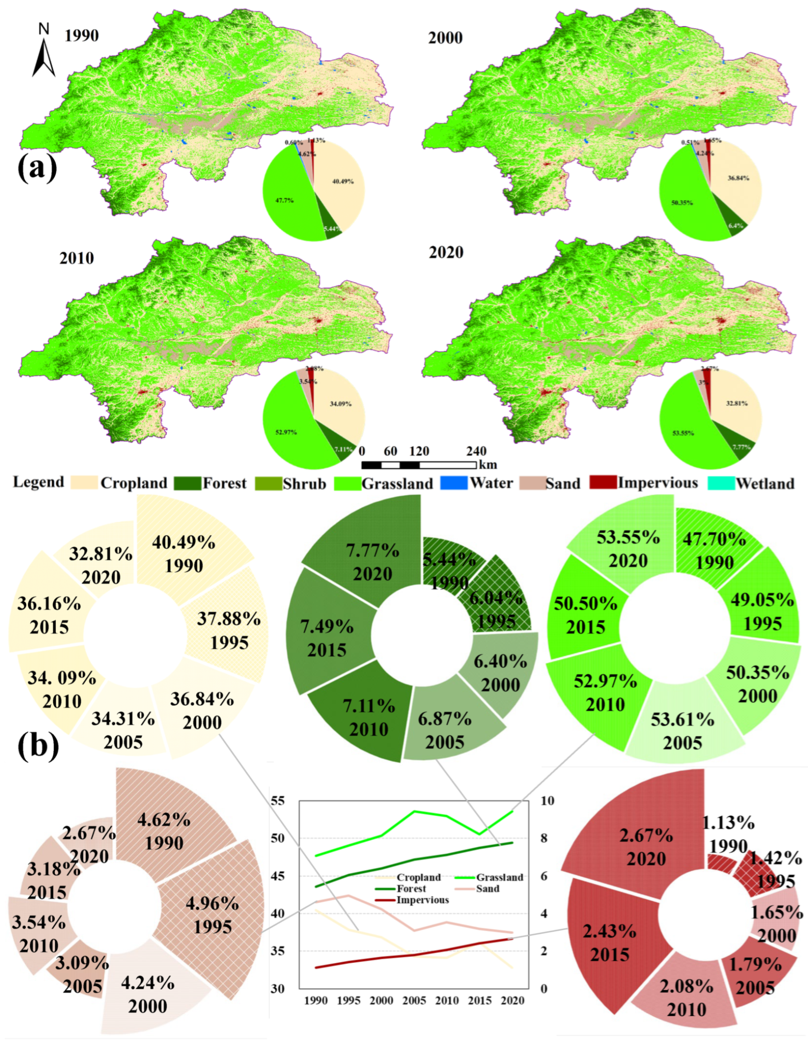
The LULC distribution maps (Figure 2a) from 1990 to 2020 revealed that forests, shrubs, and grasslands were predominantly located in the northwest and southwest regions of the basin. Compared to 1990 (53.15%, Figure 2b), vegetation cover in 2000, 2010, and 2020 showed a significant increase, accounting for 56.76%, 60.08%, and 61.32%, respectively. In contrast, cropland was mainly concentrated in the northeastern basin and the southern Horqin Sandy Land, with some areas scattered along the river. From 1990 (40.49%), cropland in the northeastern part decreased over time, accounting for 36.84%, 34.09%, and 32.81% in 2000, 2010, and 2020, respectively.
Impervious surfaces were primarily distributed along the riverbanks, interspersed with cropland. Compared to 1990, impervious areas increased by 1.13%, 1.65%, 2.08%, and 2.67% in 2000, 2010, and 2020, respectively. Notably, the central part of the WLRB contains a significant area of sandy land, the Horqin Sandy Land, which has decreased substantially from 4.62% to 2.67% of the total basin area over the past 30 years.
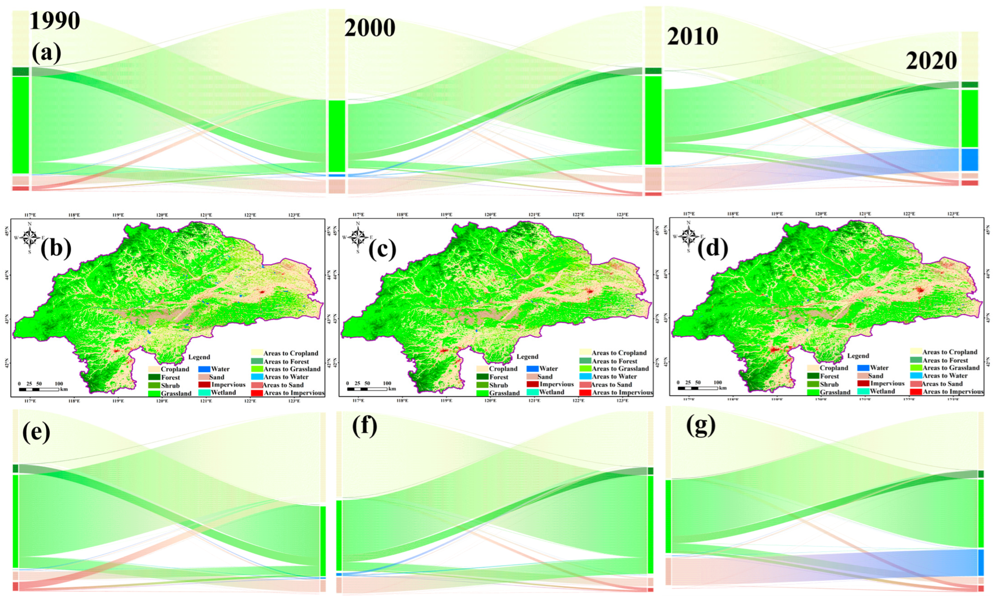
The LULC transition matrix (Figure 3) revealed that conversions between cropland and grassland made up a substantial proportion of land use changes. Specifically, the conversion of cropland to grassland accounted for 22.22% (1990–2000), 21.14% (2000–2010), and 17.80% (2010–2020), with a decreasing trend over time. These conversions were mainly clustered along the marginal zones of Horqin Sandy Land and in the southeastern part of the basin (Figure 3b–d). The conversion of grassland to cropland accounted for 11.76% (1990–2000), 10.30% (2000–2010), and 9.44% (2010–2020), while the conversion of grassland to forest accounted for 1.96% (1990–2000), 1.41% (2000–2010), and 1.25% (2010–2020). These transitions were predominantly concentrated in the south-central part of the basin. A notable transition was observed in sandy land, which was largely converted to grassland (Figure 3a,e–g). The conversion rates were 26.14%, 35.17%, and 0.13%, with the rate remaining stable during 2010–2020. Additionally, 48.48% of the sandy land was converted to water areas. The primary conversion from water was to impervious areas, with transition rates of 3.99% (1990–2000), 7.70% (2000–2010), and 8.98% (2010–2020).
As indicated by Figure 3, the transformation of grassland was primarily near cropland and sandy land, closely related to policies promoting sandy land greening and management in Horqin Sandy Land over the past decades. However, the water area has been shrinking, with some areas being converted to cropland, reflecting the trends observed in our survey. In contrast, the impervious area was expanding, which is consistent with the findings of Yang et al. [35].

3.2. Spatiotemporal Variation in Landscape Pattern Index

From 1990 to 2020, the WLRB exhibited distinct evolutionary trends. To further investigate these changes, cropland, forest, grassland, and sandy land areas with high variability were selected for detailed analysis (Table 2). During this period, the value of cropland’s PLAND, LPI, and AREA_MN decreased (from 33.83, 16.18, and 201.10 to 29.89, 13.00, and 137.91). These changes indicated that a fragmentation of the cropland, the large patches, shrunk. Conversely, the value of impervious increased, suggesting the number of patches rose. The observed changes can be attributed to shifts in LULC, as shown in Figure 2a. The LPI of forest areas increased from 0.73 to 1.40, and its AI rose from 72.92 to 74.82, indicating a consistent improvement in patch aggregation. The NP for grassland decreased from 93,883 to 91,758, although the degree of fragmentation remained relatively unchanged. In contrast, the degree of fragmentation of sandy landscapes continued to increase, with patch complexity rising, the area of large patches expanding significantly, and patch aggregation improving. Furthermore, the distribution of patches became more uniform. It is noteworthy that within the WLRB, AREA_MN of sandy land increased from 2.20 in 1990 to 3.91 in 2020, while NP decreased from 8034 to 7193. Concurrently, AI rose from 56.02 to 71.50. When considered alongside the increase in the PLAND from 0.33 to 0.52, these metrics indicate a reduction in patch count and an increase in dispersion, suggesting heightened landscape fragmentation even as total sandy area shrank. This trend is consistent with the observed spatial pattern in Figure 2a, which shows an increasingly dispersed distribution of sandy land. This pattern evolution further corroborates the effectiveness of implemented desertification control measures in the region.
Landscape changes at the watershed scale were quantified and presented in Table 3. Between 1990 and 2020, significant changes were observed in the landscape pattern indices of the WLRB. NP and ED initially decreased before increasing, reflecting an overall trend toward greater spatial fragmentation of LULC. The AREA_MN initially increased, then decreased, confirming an ongoing trend of increased fragmentation in the spatial distribution of LULC in the WLRB. The declining LPI trend suggests a gradual reduction in interactions among patch types, indicating intensified human impacts on landscape configuration, leading to more regular and aggregated patch distributions, alongside a continued decrease in overall landscape complexity.
The CONTAG initially declined slightly, followed by a sharp decrease, indicating a pronounced weakening of landscape spatial connectivity in the WLRB, particularly after 2010. The SHDI and SHEI increased from 1.2685 and 0.7080 to 1.3409 and 0.7484, respectively, reflecting a more even distribution of landscape types and an increase in landscape diversity. Over the past 30 years, landscape dominance in the WLRB progressively declined, resulting in diminished control of dominant landscape categories over the overall spatial structure (Table 3).

3.3. Obstacle Degree Analysis

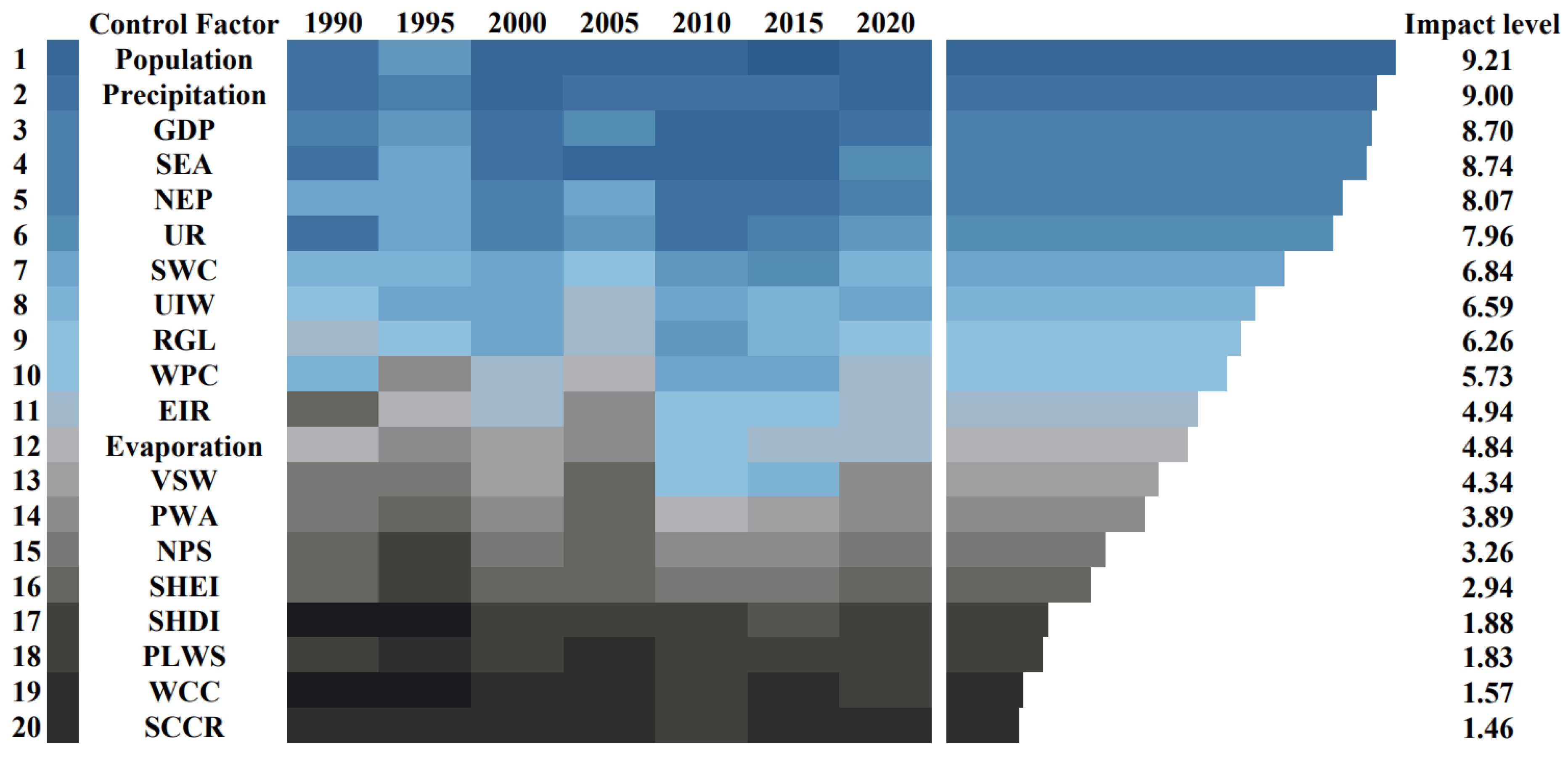
To systematically investigate the driving factors of LULC changes in the WLRB, an obstacle diagnosis model was applied to quantify the influence of 20 various factors from 1990 to 2020. The results, illustrating the influence degree of each factor, are presented in Figure 4.
Population had the highest obstacle degree (9.21) among all factors, meaning it posed the greatest hindrance to LULC changes; essentially, population pressure strongly constrained land use dynamics. Similarly, GDP had a high obstacle degree (8.70), reinforcing that economic factors were major obstacles. Precipitation and SEA emerged as the dominant factors within the indicator system of climate and socioeconomic factors, with average influence levels of 9.00 and 8.74, respectively. The population influence has exhibited an increasing trend since 1995, while precipitation showed a weakening pattern between 2005 and 2015, during which the contribution of SEA remained relatively pronounced. Overall, the socioeconomic system had a more pronounced influence on LULC changes than climate factors. The influence of the ecological environment system on LULC became significant after 2005. Notably, the impact of key internal control factors, such as the water yield coefficient, effective irrigation rate, and the flood area, increased by 21.2%, 30.5%, and 28.9%, respectively, compared to levels before 2005.
Therefore, SEM analyses should prioritize the examination of population, precipitation, GDP, SEA, NEP, UR, SWC, and UIW. It is noteworthy that these directly observed indicators, as referenced in Section 2.3.3, are categorized into three latent groups: climate change, human activities, and ecological restoration factors. Although the diagnostic analysis did not highlight the average effect of evaporation as prominent, evaporation is included in the model due to its potentially significant role within the Horqin Sandy Land catchment area.

3.4. Structural Equation Modeling Analysis

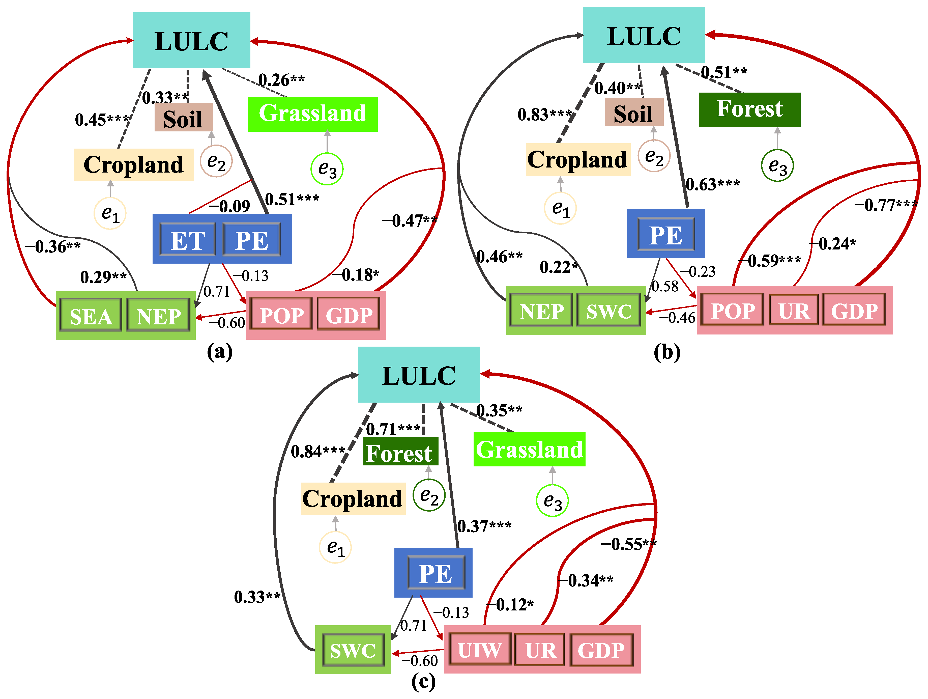
The degree of influence of natural and anthropogenic factors on LULC in the WLRB was analyzed using diagnostic models. To determine the appropriate explanatory variables, a reliability analysis of the internal control factor parameters across different groups was conducted. Based on the previous analysis, the LULC indicators for the first group selected the area proportion of cropland, soil land, and grassland (Figure 5a). The second group selected the area proportions of soil land, forest, and cropland (Figure 5b), and the third group selected the area proportions of grassland, forest, and cropland (Figure 5c). Meanwhile, we selected the observed variables of precipitation (PE) and evaporation (ET) as climate change factors; SEA, NEP, and SWC as ecological environment factors; and population (POP), GDP, UR, and UIW as human activities factors. The Cronbach’s alpha for each group met the model validation requirements.
As shown in Figure 5, the first group of factors, particularly PE, exerted positive effects on cropland, grassland, and soil land, whereas GDP and SEA had negative effects. The second group, with social factors dominated by POP, GDP, and UR, all contributed negatively, while PE, NEP, and SWC had positive effects. Similarly, the third group of socioeconomic factors, dominated by GDP and UR and UIW, all contributed negatively to the areas of cropland, grassland, and forest, while SWC and PE had positive influences.

4. Discussion

Over the past 30 years, the cropland area in the WLRB had decreased and transformed into vegetation, especially grassland. This trend is consistent with the findings of Lyu’s study [32]. Similarly, large areas of Horqin sandy land had been converted into vegetation, which was largely attributed to the implementation of soil and water conservation efforts and afforestation projects, such as the Three-North Shelterbelt Program. The reduction in water area was directly influenced by low PE and high ET in the WLRB, which aligns with the results of Li [54]. The continuous expansion of impervious surfaces along the riverbanks reflects the typical trend observed during urbanization.
Finally, forest, grassland, cropland, and sandy land were selected as representative land types to analyze the contribution of climate change, human activities, and ecological environment to LULC changes.

4.1. Effects of Climate Change on Spatiotemporal Variation in LULC

To assess the impact of climate change on LULC, we selected PE and ET for analysis. PE consistently exhibited positive impacts on LULC changes across all three groups, with significant path coefficients of 0.51, 0.63, and 0.37. A comparison between the first and second groups revealed that an increase in the path coefficient of PE was accompanied by a conversion from grassland (0.51) to forest (0.63). An increase in PE was associated with forest expansion, suggesting a positive influence of climatic factors on vegetation recovery [55]. This indicated a more pronounced response of forest to PE, likely due to their superior capacity to store water and nutrients through growth, thereby supporting more robust development [44].
Furthermore, a comparison between the second and third groups revealed that the conversion of sandy land to grassland was associated with a decrease in the contribution rate of PE. From 1990 to 2020, the conversion of sandy land to grassland in the WLRB was not primarily driven by PE, a finding consistent with prior research [56]. In contrast, the contribution of SWC increased significantly, while the negative contribution of GDP decreased. This pattern suggests that the transformation of sandy land into forestland requires substantial financial investment [57]. Similarly, a comparison between the first and third groups showed that when sandy land in the LULC was transformed into forest, the contribution rate of PE was significantly lower. These results highlight the significant role that artificial ecological restoration measures have played in reducing desertification in the WLRB [58].
The above results demonstrate that PE in the WLRB exerted a significantly positive contribution to the conversion of grassland to forestland during this period. Moreover, the impact of ET on the overall contribution rate was relatively minor compared to other factors (p > 0.05), likely because ET in the basin consistently exceeded PE during the study period, and the change was not significant [28].

4.2. Effects of Human Activities on Spatiotemporal Variation in LULC

When considering the impacts of human activities on LULC, the indicators of POP, GDP, UR, and UIW were selected. Figure 5 demonstrated that human activities had an overall adverse contribution on LULC. Among the four land types, cropland was the most outstanding, this is closely linked to the fact that urban expansion necessitates the occupation of cropland [58]. The contribution rate of GDP was higher in each group, indicating that economic development is inextricably linked to LULC changes, and rational spatial planning serves as a cornerstone for achieving high-quality watershed development [59,60].
By comparing the first and second groups, it can be found that when the LULC indicator changed from grassland to forest, the path coefficients of both GDP and POP increased significantly, from −0.47 to −0.77 (p < 0.001) and −0.18 to −0.59 (p < 0.001), respectively. The results indicate that human activities, particularly those reflected by GDP growth, exerted a negative influence on forest coverage, a trend consistent with the substantial financial investments required for afforestation efforts as noted in previous studies [61]. Comparing the second and third groups, it was observed that the negative contribution of GDP did not increase when the LULC indicator changed from sandy land to grassland. On the contrary, the UR increased, revealing that urbanization may reduce the expansion of sandy land in the basin, with increased investment [62,63]. A comparison between the first and third groups revealed that the conversion of sandy land to forest was associated with an increased proportion of cropland within the overall LULC composition.
These results further confirm that cropland had significant responds to human activities [45], especially the WLRB with a higher proportion of cropland [64,65]. Simultaneously, the increase in GDP exerts a negative contribution to the reduction in forest and grassland area.

4.3. Effects of Ecological Environment on Spatiotemporal Variation in LULC

When considering the impact of the ecological environment on LULC, SEA, NEP, and SWC were selected for analysis. NEP and SWC acted as positive contributors to the variation, whereas SEA exhibited negatively when cropland, sandy land, and grassland were selected. These results were similar to the research of Dai [65], which revelated that SEA was an important LULC indicator of desertification. A comparison between the first and second groups revealed that the contribution of NEP increased when the primary LULC type shifted from grassland to forest. This may be related to the strong carbon sink capacity of forests [66]; the increase in NEP can positively contribute to the conversion of grassland to forest.
A comparison of the second and third groups indicated that the conversion of sandy land to grassland enhanced the contribution of SWC. This suggested a close relationship between desertification control and soil-water conservation measures in the basin [67], highlighting the importance of strengthening soil conservation as a key strategy for effective sand stabilization. Simultaneously, the path coefficient of SWC increased, and that of forest also rose significantly, from 0.51 to 0.71 (p < 0.001). In the long term, this aligns with the findings of Fu’s research, suggesting that sustained ecological restoration efforts can positively contribute to the expansion of forested areas [68].

5. Conclusions

Spatiotemporal variations in LULC in the WLRB over the past 30 years were closely analyzed in this study. Notably, the area of Horqin Sandy Land consistently decreased due to the implementation of sand control measures, with much of it transforming into grassland. Meanwhile, the WLRB exhibited a trend of fragmentation, which was closely linked to human activities, particularly the influence of GDP. Precipitation acted as both a critical driver of vegetation growth and a key meteorological factor in desertification control. Therefore, integrated desertification control and rational industrial water allocation were essential for mitigating water scarcity in the basin. The findings of this study provide valuable insights for developing effective water resource management strategies in sandy areas of northern China. Furthermore, although 228 samples were constructed through sub-basin and catchment delineation, the temporal resolution of land use data was limited to 5-year intervals, thereby failing to capture seasonal dynamics. This may constrain the generalizability of the research findings. Future studies should, on the one hand, strengthen the methodologies for handling small samples by leveraging techniques such as the Jackknife and Bayesian approaches, and on the other hand, effectively utilize frequently updated time-series datasets.

Author Contributions

Conceptualization, J.L., W.L. and T.Q.; methodology, J.L. and W.L.; software, W.L.; writing—original draft, J.L., W.L. and H.L.; writing—review and editing, J.L., W.L., H.L. and T.Q.; visualization, J.L. and H.G.; validation, H.G. and H.L.; funding acquisition, T.Q. All authors have read and agreed to the published version of the manuscript.

Funding

This research was funded by “the National Science Fund Project, grant number 52130907”, “the Key Research and Development Project of Inner Mongolia autonomous region, grant number 2021ZD0015”, and “the Five Major Excellent Talent Programs of IWHR, grant number WR0199A012021”.

Data Availability Statement

Dataset available on request from the authors.

Conflicts of Interest

The authors declare no conflicts of interest.

Appendix A

Table A1. Description of landscape pattern index.
MetricsAbbreviationUnitDescription
Percent of LandscapePLANDPercentthe sum of the areas (m2) of all patches of a patch typecharacterize the area and edge metric, with higher values indicating greater landscape integrity and structural continuity
Largest Patch IndexLPIPercentthe proportion of the largest patch in total of a patch type
Edge DensityEDMeters per hectarethe sum of the lengths of all edge segments in the landscape
Mean AreaAREA_MNhathe mean of a patch type area
Fractal Dimension IndexFRAC_AMNonearea-weighted mean of fractal dimension index, quantifies the morphological complexity of patches within a landscape, wherein higher values correspond to more intricate perimeters and greater shape irregularity
Number of PatchesNPNonetotal number of patches in the landscapethe aggregation metric, higher NP reflects a heightened degree of fragmentation, lower AI signifies a more dispersed and isolated pattern
Aggregation IndexAIPercentthe degree of aggregation among landscape patches
Shannon’s Diversity IndexSHDINoneequals minus the sum (across all patch types) of the product of each patch type’s proportional abundance and its own proportionlandscape metric, a rise value is generally considered a marker of enhanced ecosystem structural stability and resilience
Shannon’s Evenness Index SHEINonea measurement determined by the distribution of different patch types within a landscape
Table A2. Description of obstacle diagnosis indicators.
Data NameAbbreviationYearData SourceDescriptionUnit
soil erosion amountSEA1990–2018National Science & Technology Infrastructure of China (http://www.nesdc.org.cn (accessed on 21 November 2023))With a resolution of 30 mt
net ecosystem productivityNEP1990–2019With a resolution of 8 kmg C m−2day−1
soil and water conservation ratioSWC1992–2019Science Data Bank
(https://cstr.cn/31253.11.sciencedb.07135 (accessed on 23 November 2023))
With a resolution of 300 mt ha−1 a−1
urbanization rateUR1990–2020Statistical YearbookCounty and township (22 counties)%
water consumption per unit of industryUIW1990–2020m3 10,000 CNY−1
effective irrigation rateEIR1990–2020%
water consumption per capitaWCC1990–2020m3
non-point source pollutionNPS1990–2020t ha−1 a−1
water production coefficientWPC1990–2020Water Resources BulletinProvincial and municipal (22 counties)%
proportion of local water supplyPLWS1990–2020%
proportion of water areaPWA1990, 2000, 2005, 2010, 2015, 2020National Geomatics Center of China (http://www.ngcc.cn/ (accessed on 12 March 2022))With a resolution of 30 mm2
Shannon’s evenness indexSHEI1990, 2000, 2005, 2010, 2015, 2020--
Shannon’s diversity indexSHDI1990, 2000, 2005, 2010, 2015, 2020--
rate of groundwater level declineRGL1990–2020Global Land Data Assimilation System (https://disc.gsfc.nasa.gov/datasets/ (accessed on 26 November 2023))With a resolution of 25 km (0–10 cm depth)m a−1
storage capacity change rateSCCR1990–2020cm
volumetric soil waterVSW1990–2020European Centre for Medium-Range Weather Forecasts Reanalysis 5 (https://apps.ecmwf.int/datasets/ (accessed on 5 December 2023))With a resolution of 3 kmm3 m−3

References

  1. Grimm, N.B.; Faeth, S.H.; Golubiewski, N.E.; Redman, C.L.; Wu, J.; Bai, X.; Briggs, J.M. Global Change and the Ecology of Cities. Science 2008, 319, 756–760. [Google Scholar] [CrossRef]
  2. Mohiuddin, G.; Mund, J.-P. Spatiotemporal Analysis of Land Surface Temperature in Response to Land Use and Land Cover Changes: A Remote Sensing Approach. Remote Sens. 2024, 16, 1286. [Google Scholar] [CrossRef]
  3. Dong, N.; You, L.; Cai, W.; Li, G.; Lin, H. Land Use Projections in China under Global Socioeconomic and Emission Scenarios: Utilizing a Scenario-Based Land-Use Change Assessment Framework. Glob. Environ. Change 2018, 50, 164–177. [Google Scholar] [CrossRef]
  4. Wang, H.; Wan, Q.; Huang, W.; Niu, J. Spatial Heterogeneity Characteristics and Driving Mechanism of Land Use Change in Henan Province, China. Geocarto Int. 2023, 38, 2271442. [Google Scholar] [CrossRef]
  5. Zhang, G.; Guhathakurta, S.; Lee, S.; Moore, A.; Yan, L. Grid-Based Land-Use Composition and Configuration Optimization for Watershed Stormwater Management. Water Resour. Manag. 2014, 28, 2867–2883. [Google Scholar] [CrossRef]
  6. Liu, M.; Tian, H. China’s Land Cover and Land Use Change from 1700 to 2005: Estimations from High-resolution Satellite Data and Historical Archives. Glob. Biogeochem. Cycles 2010, 24, 2009GB003687. [Google Scholar] [CrossRef]
  7. Wang, H.; He, M.; Ran, N.; Xie, D.; Wang, Q.; Teng, M.; Wang, P. China’s Key Forestry Ecological Development Programs: Implementation, Environmental Impact and Challenges. Forests 2021, 12, 101. [Google Scholar] [CrossRef]
  8. Chu, X.; Zhan, J.; Li, Z.; Zhang, F.; Qi, W. Assessment on Forest Carbon Sequestration in the Three-North Shelterbelt Program Region, China. J. Clean. Prod. 2019, 215, 382–389. [Google Scholar] [CrossRef]
  9. Foley, J.A.; DeFries, R.; Asner, G.P.; Barford, C.; Bonan, G.; Carpenter, S.R.; Chapin, F.S.; Coe, M.T.; Daily, G.C.; Gibbs, H.K.; et al. Global Consequences of Land Use. Science 2005, 309, 570–574. [Google Scholar] [CrossRef] [PubMed]
  10. Finér, L.; Ohashi, M.; Noguchi, K.; Hirano, Y. Factors Causing Variation in Fine Root Biomass in Forest Ecosystems. For. Ecol. Manag. 2011, 261, 265–277. [Google Scholar] [CrossRef]
  11. Cheng, Y.; Zhang, X.; Song, W. Ecological Risk Assessment of Land Use Change in the Tarim River Basin, Xinjiang, China. Land 2024, 13, 561. [Google Scholar] [CrossRef]
  12. Liu, L.; Liu, X.; Zhang, Y. Tourism-Driven Land Use Transitions and Rural Livelihood Resilience: A Spatial Production Approach to Sustainable Development in China’s Heritage Areas. Sustainability 2025, 17, 10839. [Google Scholar] [CrossRef]
  13. Liu, A.; Duodu, G.O.; Goonetilleke, A.; Ayoko, G.A. Influence of Land Use Configurations on River Sediment Pollution. Environ. Pollut. 2017, 229, 639–646. [Google Scholar] [CrossRef] [PubMed]
  14. Zhang, M.; Rong, G.; Han, A.; Riao, D.; Liu, X.; Zhang, J.; Tong, Z. Spatial-Temporal Change of Land Use and Its Impact on Water Quality of East-Liao River Basin from 2000 to 2020. Water 2021, 13, 1955. [Google Scholar] [CrossRef]
  15. Tian, M.; Hong, M.; Wang, J. Land Resources, Market-Oriented Reform and High-Quality Agricultural Development. Econ. Change Restruct. 2023, 56, 4165–4197. [Google Scholar] [CrossRef]
  16. Liu, J.; Kuang, W.; Zhang, Z.; Xu, X.; Qin, Y.; Ning, J.; Zhou, W.; Zhang, S.; Li, R.; Yan, C.; et al. Spatiotemporal Characteristics, Patterns, and Causes of Land-Use Changes in China since the Late 1980s. J. Geogr. Sci. 2014, 24, 195–210. [Google Scholar] [CrossRef]
  17. Betru, T.; Tolera, M.; Sahle, K.; Kassa, H. Trends and Drivers of Land Use/Land Cover Change in Western Ethiopia. Appl. Geogr. 2019, 104, 83–93. [Google Scholar] [CrossRef]
  18. Guo, Y.; Fang, G.; Xu, Y.-P.; Tian, X.; Xie, J. Identifying How Future Climate and Land Use/Cover Changes Impact Streamflow in Xinanjiang Basin, East China. Sci. Total Environ. 2020, 710, 136275. [Google Scholar] [CrossRef] [PubMed]
  19. Yao, Z.; Wang, B.; Huang, J.; Zhang, Y.; Yang, J.; Deng, R.; Yang, Q. Analysis of Land Use Changes and Driving Forces in the Yanhe River Basin from 1980 to 2015. J. Sens. 2021, 2021, 6692333. [Google Scholar] [CrossRef]
  20. Zhang, S.; Guan, Z.; Liu, Y.; Zheng, F. Land Use/Cover Change and Its Relationship with Regional Development in Xixian New Area, China. Sustainability 2022, 14, 6889. [Google Scholar] [CrossRef]
  21. Lin, F.; Chen, X.; Yao, H.; Lin, F. SWAT Model-Based Quantification of the Impact of Land-Use Change on Forest-Regulated Water Flow. Catena 2022, 211, 105975. [Google Scholar] [CrossRef]
  22. Wei, X.; Ye, Y.; Zhang, Q.; Fang, X. Methods for Cropland Reconstruction Based on Gazetteers in the Qing Dynasty (1644–1911): A Case Study in Zhili Province, China. Appl. Geogr. 2015, 65, 82–92. [Google Scholar] [CrossRef]
  23. Dick, G.; Schumacher, M.V.; Momolli, D.R.; Viera, M. Nutrient Input via Incident Rainfall in a Eucalyptus Dunnii Stand in the Pampa Biome. Floresta E Ambiente 2018, 25, e20160559. [Google Scholar] [CrossRef]
  24. Han, J.; Wang, J.; Chen, L.; Xiang, J.; Ling, Z.; Li, Q.; Wang, E. Driving Factors of Desertification in Qaidam Basin, China: An 18-Year Analysis Using the Geographic Detector Model. Ecol. Indic. 2021, 124, 107404. [Google Scholar] [CrossRef]
  25. Wang, Y.; Jiang, R.; Yang, M.; Xie, J.; Zhao, Y.; Li, F.; Lu, X. Spatiotemporal characteristics and driving mechanisms of land use/land cover (LULC) changes in the Jinghe River Basin, China. J. Arid. Land 2024, 16, 91–109. [Google Scholar] [CrossRef]
  26. Luo, J.; Xin, L.; Liu, F.; Chen, Q.; Zhou, Q.; Zhang, Y. Study of the Intensity and Driving Factors of Land Use/Cover Change in the Yarlung Zangbo River, Nyang Qu River, and Lhasa River Region, Qinghai-Tibet Plateau of China. J. Arid. Land. 2022, 14, 411–425. [Google Scholar] [CrossRef]
  27. Wang, Y.; Liu, X.; Wang, T.; Zhang, X.; Feng, Y.; Yang, G.; Zhen, W. Relating Land-Use/Land-Cover Patterns to Water Quality in Watersheds Based on the Structural Equation Modeling. Catena 2021, 206, 105566. [Google Scholar] [CrossRef]
  28. Ye, G.; Chen, K.; Yang, Y.; Liang, S.; Hu, W.; He, L. Integrative Framework for Decoding Spatial and Temporal Drivers of Land Use Change in Malaysia: Strategic Insights for Sustainable Land Management. Land 2024, 13, 2248. [Google Scholar] [CrossRef]
  29. Sui, L.; Yan, Z.; Li, K.; Wang, C.; Shi, Y.; Du, Y. Prediction of Ecological Security Network in Northeast China Based on Landscape Ecological Risk. Ecol. Indic. 2024, 160, 111783. [Google Scholar] [CrossRef]
  30. Zhou, T.; Shen, W.; Qiu, X.; Chang, H.; Yang, H.; Yang, W. Impact Evaluation of a Payments for Ecosystem Services Program on Vegetation Quantity and Quality Restoration in Inner Mongolia. J. Environ. Manag. 2022, 303, 114113. [Google Scholar] [CrossRef]
  31. Zhang, G.; Kang, Y.; Han, G.; Sakurai, K. Effect of Climate Change over the Past Half Century on the Distribution, Extent and NPP of Ecosystems of Inner Mongolia: Effect Of Climate Change On The Ecosystem. Glob. Change Biol. 2011, 17, 377–389. [Google Scholar] [CrossRef]
  32. Lyu, X.; Li, X.; Wang, K.; Dang, D.; Gong, J.; Wang, H.; Lou, A. Optimizing Landscape Patterns to Maximize Ecological-production Benefits of Water–Food Relationship: Evidence from the West Liaohe River Basin, China. Land Degrad. Dev. 2023, 34, 3388–3405. [Google Scholar] [CrossRef]
  33. Xu, W.; Meng, L.; Liu, P.; Dong, K. Use of a Modified Chloride Mass Balance Technique to Assess the Factors That Influence Groundwater Recharge Rates in a Semi-Arid Agricultural Region in China. Environ. Earth Sci. 2019, 78, 241. [Google Scholar] [CrossRef]
  34. Zhu, Y.; Zhang, S.; Luo, P.; Su, F.; Sun, B.; Liang, L.; Guo, J.; Yang, R. Assessing Ecohydrological Factors Variations and Their Relationships at Different Spatio-Temporal Scales in Semiarid Area, Northwestern China. Adv. Space Res. 2021, 67, 2368–2381. [Google Scholar] [CrossRef]
  35. Yang, X.; Ren, L.; Liu, Y.; Jiao, D.; Jiang, S. Hydrological Response to Land Use and Land Cover Changes in a Sub-Watershed of West Liaohe River Basin, China. J. Arid. Land 2014, 6, 678–689. [Google Scholar] [CrossRef]
  36. Wang, K.; Li, X.; Lyu, X.; Dang, D.; Dou, H.; Li, M.; Liu, S.; Cao, W. Optimizing the Land Use and Land Cover Pattern to Increase Its Contribution to Carbon Neutrality. Remote Sens. 2022, 14, 4751. [Google Scholar] [CrossRef]
  37. Li, W.; Liu, S.; Chang, W.; Zhang, X.; Li, C.; Qin, T. Research Progress on the Evaluationof Water Resources Carrying Capacity. Pol. J. Environ. Stud. 2023, 32, 1975–1986. [Google Scholar] [CrossRef]
  38. Shao, T.; Liang, X.; Zhuang, D.; Zheng, K.; Wang, T. Seasonal Variations in CDOM Characteristics and Effects of Environmental Factors in Coastal Rivers, Northeast China. Environ. Sci. Pollut. Res. 2022, 30, 29052–29064. [Google Scholar] [CrossRef]
  39. Yang, J.; Huang, X. The 30 m Annual Land Cover Dataset and Its Dynamics in China from 1990 to 2019. Earth Syst. Sci. Data 2021, 13, 3907–3925. [Google Scholar] [CrossRef]
  40. Huang, D.; Wen, F.; Li, G.; Wang, Y. Coupled Development of the Urban Water-Energy-Food Nexus: A Systematic Analysis of Two Megacities in China’s Beijing-Tianjin-Hebei Area. J. Clean. Prod. 2023, 419, 138051. [Google Scholar] [CrossRef]
  41. Yi, D.; Ding, G.; Han, Y.; Yi, J.; Guo, J.; Ou, M. Integrated Assessment and Critical Obstacle Diagnosis of Rural Resource and Environmental Carrying Capacity with a Social–Ecological Framework: A Case Study of Liyang County, Jiangsu Province. Environ. Sci. Pollut. Res. 2023, 30, 76026–76043. [Google Scholar] [CrossRef]
  42. Li, J.; Liu, S.; Chen, J.; Zhao, Y.; Abebe, S.A.; Dong, B.; Wang, W.; Qin, T. Response of Stream Water Quality to the Vegetation Patterns on Arid Slope: A Case Study of Huangshui River Basin. Environ. Sci. Pollut. Res. 2024, 31, 9167–9182. [Google Scholar] [CrossRef]
  43. López, E.; Bocco, G.; Mendoza, M.; Duhau, E. Predicting Land-Cover and Land-Use Change in the Urban Fringe. Landsc. Urban Plan. 2001, 55, 271–285. [Google Scholar] [CrossRef]
  44. Zhang, Z.; Zhang, L.; Xu, H.; Creed, I.F.; Blanco, J.A.; Wei, X.; Sun, G.; Asbjornsen, H.; Bishop, K. Forest Water-Use Efficiency: Effects of Climate Change and Management on the Coupling of Carbon and Water Processes. For. Ecol. Manag. 2023, 534, 120853. [Google Scholar] [CrossRef]
  45. McGarigal, K.; Cushman, S.A.; Neel, M.C.; Ene, E. Fragstats: Spatial Pattern Analysis Program for Categorical Maps. 2002. Available online: www.umass.edu/landeco/research/fragstats/fragstats.html (accessed on 23 April 2025).
  46. Deng, J.S.; Wang, K.; Hong, Y.; Qi, J.G. Spatio-Temporal Dynamics and Evolution of Land Use Change and Landscape Pattern in Response to Rapid Urbanization. Landsc. Urban. Plan. 2009, 92, 187–198. [Google Scholar] [CrossRef]
  47. Wu, J.; Luo, J.; Zhang, H.; Yu, M. Driving Forces behind the Spatiotemporal Heterogeneity of Land-Use and Land-Cover Change: A Case Study of the Weihe River Basin, China. J. Arid. Land 2023, 15, 253–273. [Google Scholar] [CrossRef]
  48. Sun, S.; Chen, H.; Ju, W.; Song, J.; Zhang, H.; Sun, J.; Fang, Y. Effects of Climate Change on Annual Streamflow Using Climate Elasticity in Poyang Lake Basin, China. Theor. Appl. Climatol. 2013, 112, 169–183. [Google Scholar] [CrossRef]
  49. Wang, L.; Wang, N.; Pang, M.; Zhang, Q.; Wei, D.; Li, Y.; An, Z.; Jin, L. Analysis of Spatiotemporal Land Use Change Characteristics in the Upper Watershed Area of the Qingshui River Basin from 1990 to 2020. Front. Environ. Sci. 2024, 12, 1388058. [Google Scholar] [CrossRef]
  50. Zheng, Y.; Wang, Z.; Li, S.; Zheng, Z.; Wang, F.; Zhao, X.; He, J.; Ji, D.; Wang, W. Analysis of Spatiotemporal Dynamic Evolution Characteristics and Driving Forces of Land Use/Cover Change in the Weihe River Basin in the Past 30 Years. Environ. Sci. 2025, 46, 7106–7118. (In Chinese) [Google Scholar] [CrossRef]
  51. Liu, J.; Wang, Z.; Duan, Y.; Li, X.; Zhang, M.; Liu, H.; Xue, P.; Gong, H.; Wang, X.; Chen, Y.; et al. Effects of Land Use Patterns on the Interannual Variations of Carbon Sinks of Terrestrial Ecosystems in China. Ecol. Indic. 2023, 146, 109914. [Google Scholar] [CrossRef]
  52. Desta, G.; Abera, W.; Tamene, L.; Amede, T. A Meta-Analysis of the Effects of Land Management Practices and Land Uses on Soil Loss in Ethiopia. Agric. Ecosyst. Environ. 2021, 322, 107635. [Google Scholar] [CrossRef]
  53. Wang, J.; Li, Z.; Yu, Y.; Shen, Z.; Wang, Y.; Zhang, H. Seasonally Disparate Responses of Surface Thermal Environment to Land Use/Land Cover Patterns: A Case Study of Central Urban Area of Jinan City, China. Int. J. Biometeorol. 2025, 69, 2983–2997. [Google Scholar] [CrossRef]
  54. Li, J.; Xu, B.; Yang, X.; Qin, Z.; Zhao, L.; Jin, Y.; Zhao, F.; Guo, J. Historical Grassland Desertification Changes in the Horqin Sandy Land, Northern China (1985–2013). Sci. Rep. 2017, 7, 3009. [Google Scholar] [CrossRef]
  55. Liu, Y.; Shang, Z.; Li, L.; Jiang, H.; Jia, B.; Liu, J.; Ren, H.; Zhu, Y. Spatiotemporal Variation of Vegetation Cover and Land Use in the Upper Xiliao River Basin and Its Impact on River Sediment Concentration. China Rural. Water Hydropower 2025, 1–15. (In Chinese) [Google Scholar]
  56. Mganga, K.Z.; Musimba, N.K.R.; Nyariki, D.M.; Nyangito, M.M.; Mwang’ombe, A.W. The Choice of Grass Species to Combat Desertification in Semi-arid Kenyan Rangelands Is Greatly Influenced by Their Forage Value for Livestock. Grass Forage Sci. 2015, 70, 161–167. [Google Scholar] [CrossRef]
  57. Yang, B.; Wang, Q.; Xu, X. Evaluation of Soil Loss Change after Grain for Green Project in the Loss Plateau: A Case Study of Yulin, China. Environ. Earth Sci. 2018, 77, 304. [Google Scholar] [CrossRef]
  58. Liu, D.; Chen, J.; Ouyang, Z. Responses of Landscape Structure to the Ecological Restoration Programs in the Farming-Pastoral Ecotone of Northern China. Sci. Total Environ. 2020, 710, 136311. [Google Scholar] [CrossRef] [PubMed]
  59. Peng, C.; Song, M.; Han, F. Urban Economic Structure, Technological Externalities, and Intensive Land Use in China. J. Clean. Prod. 2017, 152, 47–62. [Google Scholar] [CrossRef]
  60. Asante-Yeboah, E.; Koo, H.; Ros-Tonen, M.A.F.; Sieber, S.; Fürst, C. Participatory and Spatially Explicit Assessment to Envision the Future of Land-Use/Land-Cover Change Scenarios on Selected Ecosystem Services in Southwestern Ghana. Environ. Manag. 2024, 74, 94–113. [Google Scholar] [CrossRef]
  61. Kung’u, G.N.; Cousseau, L.; Githiru, M.; Habel, J.C.; Kinyanjui, M.; Matheka, K.; Schmitt, C.B.; Seifert, T.; Teucher, M.; Lens, L.; et al. Anthropogenic Activities Affect Forest Structure and Arthropod Abundance in a Kenyan Biodiversity Hotspot. Biodivers. Conserv. 2023, 32, 3255–3282. [Google Scholar] [CrossRef]
  62. Nassar, A.K.; Alan Blackburn, G.; Duncan Whyatt, J. Developing the Desert: The Pace and Process of Urban Growth in Dubai. Comput. Environ. Urban 2014, 45, 50–62. [Google Scholar] [CrossRef]
  63. Droomers, M.; Jongeneel-Grimen, B.; Bruggink, J.-W.; Kunst, A.; Stronks, K. Is It Better to Invest in Place or People to Maximize Population Health? Evaluation of the General Health Impact of Urban Regeneration in Dutch Deprived Neighbourhoods. Health Place 2016, 41, 50–57. [Google Scholar] [CrossRef]
  64. Shi, X.; Wang, W.; Shi, W. Progress on Quantitative Assessment of the Impacts of Climate Change and Human Activities on Cropland Change. J. Geogr. Sci. 2016, 26, 339–354. [Google Scholar] [CrossRef]
  65. Dai, Y.; Tian, L.; Zhu, P.; Dong, Z.; Zhang, R. Dynamic Aeolian Erosion Evaluation and Ecological Service Assessment in Inner Mongolia, Northern China. Geoderma 2022, 406, 115518. [Google Scholar] [CrossRef]
  66. Ke, S.; Zhang, Z.; Wang, Y. China’s Forest Carbon Sinks and Mitigation Potential from Carbon Sequestration Trading Perspective. Ecol. Indic. 2023, 148, 110054. [Google Scholar] [CrossRef]
  67. Bogunović, I.; Kovács, P.G.; Ðekemati, I.; Kisić, I.; Balla, I.; Birkás, M. Long-Term Effect of Soil Conservation Tillage on Soil Water Content, Penetration Resistance, Crumb Ratio and Crusted Area. Plant Soil Environ. 2019, 65, 442–448. [Google Scholar] [CrossRef]
  68. Fu, B.; Wang, S.; Liu, Y.; Liu, J.; Liang, W.; Miao, C. Hydrogeomorphic Ecosystem Responses to Natural and Anthropogenic Changes in the Loess Plateau of China. Annu. Rev. Earth Planet. Sci. 2017, 45, 223–243. [Google Scholar] [CrossRef]
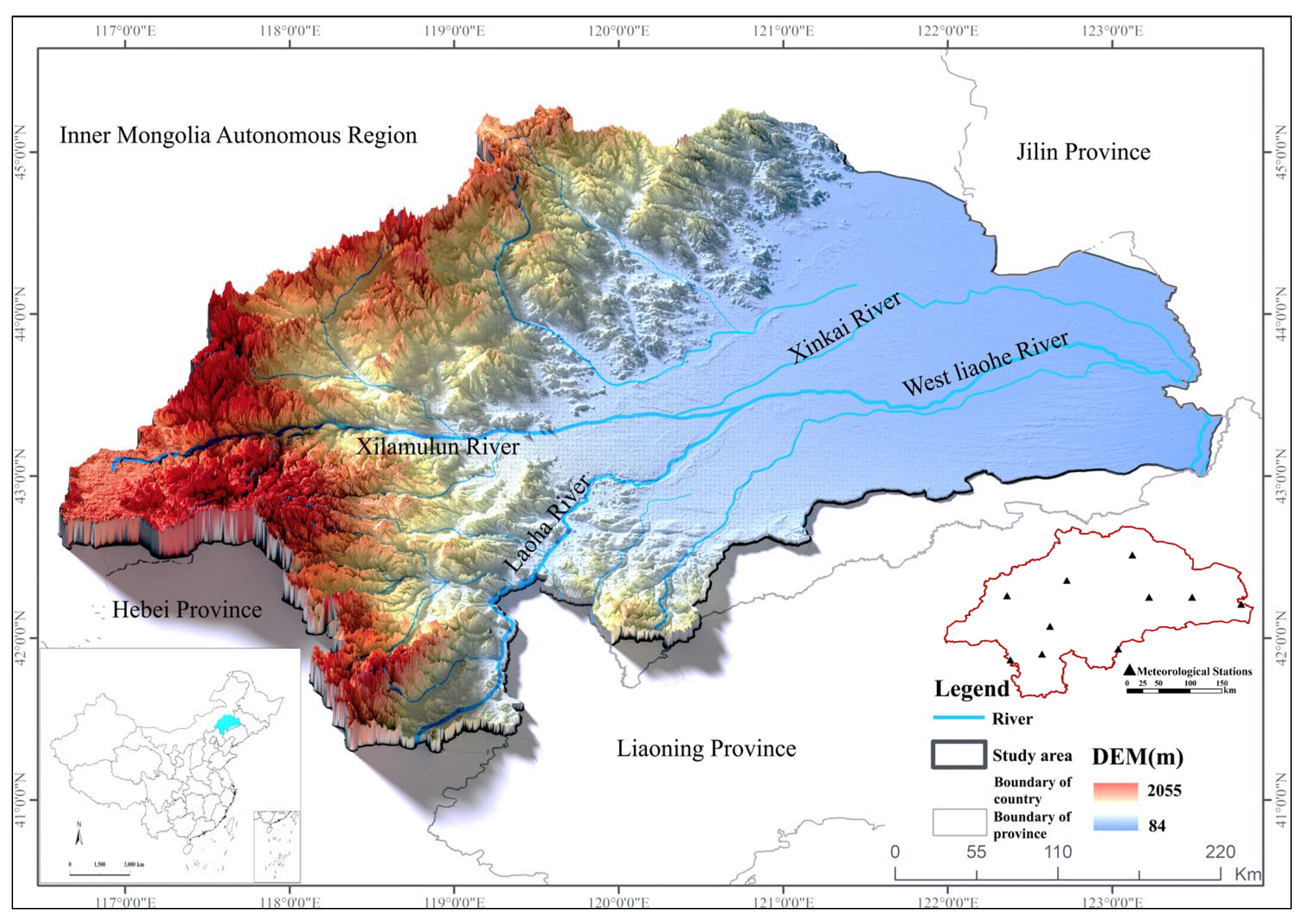
Figure 1. Overview of the WLRB.
Hydrology 13 00042 g001
Figure 2. Spatiotemporal distributions of LULC in the WLRB: (a) spatial distribution of land use changes per decade and (b) temporal trends (line graph and pie chart).
Hydrology 13 00042 g002
Figure 3. Transition matrix of LULC from 1990 to 2000 (b), from 2000 to 2010 (c), from 2010 to 2020 (d) in the WLRB ((a,eg) represent Sankey diagrams of land use change; (a) illustrates the entire 30-year period, while (eg) depict the three separate decadal intervals, respectively).
Hydrology 13 00042 g003
Figure 4. Obstacle degree analysis results of WLRB from 1990 to 2020 (the names, abbreviations, data sources, and temporal aggregation for the 20 indicators are provided in the Table A2 of the Appendix A).
Hydrology 13 00042 g004
Figure 5. SEM results of WLRB in different groups. ((a)–(c) represent the path coefficients between three latent variables and different LULC. The gray arrow represents positive effects and the red one indicates negative effects. The numbers on the line indicate influence coefficients: * p < 0.05, ** p < 0.01, *** p < 0.001. Each groups’ CFI were greater than 0.88, and RMSEA were less than 0.087. The model was considered to pass).
Hydrology 13 00042 g005
Table 1. Data types, sources, and description.
Data NameYearData SourceDescription
Precipitation1990–2020China Meteorological Data Service Center (http://data.cma.cn/ (accessed on 9 August 2023))Daily data from 10 meteorological
stations
Evaporation
Population1990–2020Statistical YearbookCounty and township (22 counties)
GDP
Industry structures
Land use1990, 2000, 2005, 2010, 2015, 2020National Geomatics Center of China (http://www.ngcc.cn/ (accessed on 12 March 2022))With a resolution of 30 m
Water Resources1990–2020Water Resources BulletinProvincial and municipal (22 counties)
Soil Moisture1990–2020Global Land Data Assimilation System (https://disc.gsfc.nasa.gov/datasets/ (accessed on 20 November 2023))With a resolution of 25 km (0–10 cm depth)
Table 2. Landscape pattern index of different types in WLRB from 1990 to 2020.
TypesYearPLANDLPIEDAREA_MNFRAC_AMNPAI
Cropland199033.8316.1817.12201.101.3182907192.41
201031.9815.0217.40161.511.310510,67691.84
202029.8913.0017.53137.911.304511,68591.21
Forest199022.820.7341.1610.591.299116,23972.92
201023.191.1340.8410.271.2974121,79873.56
202024.001.4040.2510.921.2968118,52374.82
Grassland199038.2115.0549.9521.941.359893,88380.36
201038.7915.4449.5122.261.366993,95580.83
202037.8314.4448.4122.231.361791,75880.77
Water19901.9171.101.3214.331.1674721589.39
20102.091.111.1026.721.1754421391.84
20201.960.551.1244.401.1637238291.19
Impervious19902.890.113.2425.681.1064607783.23
20103.650.243.65 26.341.1112747285.02
20205.800.295.5333.911.1363922785.69
Sandy land19900.330.020.962.201.1305803456.02
20100.310.010.961.981.1241838153.33
20200.520.031.003.911.1247719371.50
Table 3. Landscape pattern index variations in WLRB from 1990 to 2020.
YearNPLPIEDAREA_MNCONTAGSHDISHEI
1990240,51916.184956.883122.418553.71811.26850.7080
2010246,49515.443256.729321.875753.0421.29020.7201
2020240,76814.435356.925322.395747.25241.34090.7484
Note: NP and LPI were selected to discuss the dominant landscape types and the interannual changes; ED and AREA_MN discussed the degree of watershed landscape fragmentation; CONTAG were used to discuss the correlation of dominant landscape type; SHDI and SHEI were used to reflect the changes in landscape diversity in different periods in the area.
Disclaimer/Publisher’s Note: The statements, opinions and data contained in all publications are solely those of the individual author(s) and contributor(s) and not of MDPI and/or the editor(s). MDPI and/or the editor(s) disclaim responsibility for any injury to people or property resulting from any ideas, methods, instructions or products referred to in the content.